Methods for Time Dependence in DMRG

Abstract

A major advance in density-matrix renormalization group (DMRG) calculations has been achieved by the invention of highly efficient DMRG techniques for the simulation of real-time dynamics of strongly correlated quantum systems in one dimension. Starting from established linear-response techniques in DMRG and early attempts at real-time dynamics, we go on to review two current methods which both implement the idea of adapting the effective Hilbert space of DMRG to the quantum state evolving in time. We also give an outlook on extensions to finite temperature calculations.

1 Introduction

The physics of strongly correlated quantum systems continues to pose major challenges in experimental and theoretical physics. While both experiment and theory have focused on static, thermodynamic or at most linear-response quantities in the past, recently questions which explicitly involve the out-of-equilibrium time-dependence of such quantum systems have come to the foreground. These questions arise in the context of transport far from equilibrium or of decoherence, particularly as the size of devices continues to shrink towards the atomic scale. However, perhaps the most striking example for this is provided by the progress in preparing dilute ultracold bosonic and also fermionic alkali gases. Subjected to an optical lattice, these gases are arguably the purest realization of the typical model Hamiltonians of strong correlation physics, such as the Hubbard modelGrei02 ; Kohl05 . More importantly, the interaction parameters can be tuned experimentally on quantum mechanically relevant time-scales over a huge range, while being known precisely from microscopic calculations. From a theoretician’s point of view, this situation is almost ideal, and has stimulated great interest in the development of time-dependent methods.

For linear response, exact diagonalization can provide detailed results for small systems, and quantum Monte Carlo can provide coarse resolution results after analytic continuation from imaginary time, for systems without the sign problem. Outside the linear response regime, almost the only tool available has been the diagonalization of very small clusters.

In this review, the emphasis is on recent extensions of the density-matrix renormalization group method (DMRG) Whit92 ; Whit93 ; Scho04 into the real-time domain which make it the currently most powerful method for such problems. Following up on early attempts to extend DMRG to real-time, input from quantum information theory has led to the formulation of two DMRG algorithms for real-time evolutions. We set out with a reminder about the basic ideas of DMRG, review linear response calculations with DMRG and move on to early attempts in the time domain. We then explain how the TEBD algorithm of Vidal Vida04 beautifully reflects fundamental structures of DMRG and hence can be easily used to extend DMRG to the time-domain Dale04 ; Whit04 . However, this approach has shortcomings for longer-ranged interactions, which can be circumvented in yet another modification of DMRG at some cost in efficiency Whit04c . The range and power of both methods are discussed based on “real-life” applications.

2 Basic Ideas of DMRG

Several good descriptions of the DMRG algorithms exist in the literature Whit92 ; Whit93 ; Scho04 . Rather than repeat these descriptions, here we summarize the most important ideas of DMRG.

The first key idea is the description of a collection of sites, or block, in terms of a limited set of basis states and operator matrices between those states. These states and matrices are defined by a set of basis transformations as sites are successively added to the block. This representation is due to Wilson and is a key feature of his numerical renormalization group (NRG)Wils75 . Let the block at the beginning of step $\ell$ be described by a set of states $\{|i\rangle\}$. In this step site $\ell$ (states $\{|\sigma\rangle\}$) is added to the block. The new states describing the larger block $\{|i^{\prime}\rangle\}$ are given by

$$|i^{\prime}\rangle=\sum_{\sigma,i}A^{\ell}_{ii^{\prime}}[\sigma]|i\rangle\otimes|\sigma\rangle.$$

The number of states is kept approximately constant at $m$, so the set of states $\{|i^{\prime}\rangle\}$ is incomplete. If the states $\{|i^{\prime}\rangle\}$ were described in detail in terms of the sites, the computational effort would grow exponentially despite the truncation to a constant number of states. Instead, the $m\times m$ matrices for the Hamiltonian and other operators give all the detail needed to construct the Hamiltonian at larger length scales. These matrices are transformed to the new basis at each step using the transformation matrices $A$. In this way, the computational effort remains constant as $O(m^{3})$.

The second key idea of DMRG is to choose the states to keep as eigenstates of the reduced density matrix (RDM) of the block. In Wilson’s NRG approach, one kept the lowest energy eigenstates of the block Hamiltonian. This choice works for the special Hamiltonians devised by Wilson for impurity systems, but fails for more general lattice systems. Using the density matrix eigenstates can be shown to be optimal for reproducing the wavefunction as well as the RDM. Let the block have states $|i\rangle$ and the rest of the system, referred to as the environment, have states $|j\rangle$. Then the wavefunction of the whole system is written as

$$|\psi\rangle=\sum_{ij}\psi_{ij}|i\rangle\otimes|j\rangle$$

and the coefficients of the RDM $\rho$ are

$$\rho_{ii^{\prime}}=\sum_{j}\psi_{ij}\psi^{*}_{i^{\prime}j}.$$

The eigenvalues of $\rho$ are the probabilities of the block being in the corresponding eigenstate, and if the probability is neglible, the eigenstate can be omitted from the basis. The RDM can also be built by summing over several states $|\psi^{a}\rangle$, with arbitrary weights, representing the probability of each $\psi^{a}$ in a mixed state of the system. In this case each $|\psi^{a}\rangle$ is said to be targetted, an important concept for time-dependent DMRG.

The RDM depends on the enviroment through $|\psi\rangle$. In DMRG, both the block and the environment are described approximately using basis sets of size $\sim m$. This leads to the third key idea of DMRG, the idea of sweeping back and forth to produce a self-consistent, accurate representation for both parts of the system. In Fig. 1 we show the most common superblock configuration in DMRG. In the sweeping procedure the dividing line between the left and right block moves back and forth between the ends of the system. The block which is growing is treated as the system block; the other is the enviroment, with the roles reversed when the direction is reversed. The system block in each case obtains an improved basis during the sweep. In Wilson’s NRG, there was no sweeping and no feedback from the low energy scales to the high energy scales. For a general lattice system, not divided by energy scales, feedback is necessary.

Figure 1: The standard DMRG superblock configuration, in which the left central site is being added onto the left block.

If we trace back through the basis set transformations which led to the basis of a block, one obtains an explicit representation of the states

$$|i_{\ell}\rangle=\sum_{\sigma_{1}\ldots\sigma_{\ell}}[A^{1}[\sigma_{1}]A^{2}[\sigma_{2}]\ldots A^{\ell}[\sigma_{\ell}]]_{i_{\ell}}|\sigma_{1}\ldots\sigma_{\ell}\rangle$$

where $A^{1}$ is a vector for each $\sigma_{1}$ and the rest of the $A$’s are matrices. We can write the basis states for the right block similarly. Alternatively, we can let the dividing line be all the way on the right end of the system, in which case we can write the following matrix product expression for $|\psi\rangle$:

$$|\psi\rangle=\sum_{\sigma_{1}\ldots\sigma_{L}}A^{1}[\sigma_{1}]A^{2}[\sigma_{2}]\ldots A^{L}[\sigma_{L}]|\sigma_{1}\ldots\sigma_{L}\rangle$$

where $A^{L}[\sigma_{L}]$ is a vector for each value of $\sigma_{L}$, so that the product of the $A$’s is a scalar. The matrix product representation for $|\psi\rangle$ was first developed in a DMRG context by Ostlund and RommerOstl95 , but its usefulness was not widely appreciated at the time. More recently, the matrix product representation has become very important as a route to improve the capabilities of and to generalize DMRG Vers04 .

Figure 2: Diagrams for the matrix product representation of the wavefunction and an operator on a block.

A useful diagrammatic form of the matrix product representation Vers04 is illustrated in Fig. 2. The upper diagram represents the wavefunction. Here each intersection of lines is associated with a site and represents a matrix (here the $A^{\ell}[\sigma_{\ell}]$), or more generally, a tensor. The vectors $A^{1}$ and $A^{L}$ are reprecented by right-angle segments. Interior line segments represent indices which are summed over, whereas the ends of segments sticking out of the figure represent external indices labeling states. As another example, let an operator $\hat{O}$ be defined as a product of site operators on the left block, $\hat{O}_{1}\ldots\hat{O}_{\ell}$, where many of the $\hat{O}_{i}$ may be identity operators. The lower diagram represents the matrix for this operator in the basis of the left block. Each of the two lines sticking out on the right represents indices running over the $m$ states of the left block.

3 DMRG dynamics

While the original DMRG algorithm seems to be limited to the calculation of equilibrium properties such as ground state correlations, it can in fact be extended to linear response quantities. For some operator $\hat{A}$, we define a (time-dependent) Green’s function at $T=0$ in the Heisenberg picture by

$${\rm i}G_{A}(t^{\prime}-t)=\langle 0|\hat{A}^{\dagger}(t^{\prime})\hat{A}(t)|0\rangle$$ (1)

with $t^{\prime}\geq t$ for a time-independent Hamiltonian $\hat{H}$. Going to frequency-space, the Green’s function reads

$$G_{A}(\omega+{\rm i}\eta)=\langle 0|\hat{A}^{\dagger}\frac{1}{E_{0}+\omega+{\rm i}\eta-\hat{H}}\hat{A}|0\rangle,$$ (2)

where $\eta$ is some positive number to be taken to zero at the end. We may also use the spectral or Lehmann representation of correlations in the eigenbasis of $\hat{H}$,

$$C_{A}(\omega)=\sum_{n}|\langle n|\hat{A}|0\rangle|^{2}\delta(\omega+E_{0}-E_{n}).$$ (3)

$C_{A}(\omega)$ is related to $G_{A}(\omega+{\rm i}\eta)$ as

$$C_{A}(\omega)=\lim_{\eta\rightarrow 0^{+}}-\frac{1}{\pi}{\rm Im}G_{A}(\omega+{\rm i}\eta).$$ (4)

The role of $\eta$ in DMRG calculations is threefold: First, it ensures causality in Eq. (2). Second, it introduces a finite lifetime $\tau\propto 1/\eta$ to excitations. Third, $\eta$ provides a Lorentzian broadening of $C_{A}(\omega)$,

$$C_{A}(\omega+{\rm i}\eta)=\frac{1}{\pi}\int d\omega^{\prime}C_{A}(\omega^{\prime})\frac{\eta}{(\omega-\omega^{\prime})^{2}+\eta^{2}},$$ (5)

which serves either to broaden the numerically obtained discrete spectrum of finite systems into some “thermodynamic limit” behavior or to broaden analytical results for $C_{A}$ for comparison to numerical spectra where $\eta>0$.

Most DMRG approaches to dynamical correlations center on the evaluation of Eq. (2). The first, which we refer to as Lanczos vector dynamics, has been pioneered by Hallberg Hall95 , and calculates highly time-efficient, but comparatively rough approximations to dynamical quantities adopting the Balseiro-Gagliano method Gagl87 to DMRG. The second class of approaches, including both the correction vector method Rama97 ; Kuhn99 and DDMRG (dynamical DMRG) Jeck02 , is also based on pre-DMRG techniques, but is both much more precise and numerically much more expensive.

Boundary effects due to DMRG-typical open boundary conditions can be treated in various ways; two situations should be distinguished. If $\hat{A}$ acts locally, such as in the calculation of an optical conductivity, one may exploit that finite $\eta$ exponentially suppresses excitations Jeck02 . As they travel at some speed $c$ through the system, a thermodynamic limit $L\rightarrow\infty$ first, $\eta\rightarrow 0$ second may be taken consistently as a single limit with $\eta=c/L$. For the calculation of dynamical structure functions such as obtained in elastic neutron scattering, $\hat{A}$ is a spatially delocalized Fourier transform, and another approach must be taken. The open boundaries introduce both genuine edge effects and a hard cut to the wave functions of excited states in real space, leading to a large spread in momentum space. To limit bandwidth in momentum space, filtering by modifying $\hat{A}(x)\rightarrow\hat{A}(x)f(x)$ is necessary. The filtering function $f(x)$ should be narrow in momentum space and broad in real space, while simultaneously strictly excluding edge sites. For a detailed discussion of such filters, see Kuhn99 .

3.1 Continued fraction dynamics

The technique of continued fraction dynamics has first been exploited by Gagliano and Balseiro Gagl87 in the framework of exact ground state diagonalization. Obviously, the calculation of Green’s functions as in Eq. (2) involves the inversion of $\hat{H}$ (or more precisely, $E_{0}+\omega+{\rm i}\eta-\hat{H}$), a typically very large sparse hermitian matrix. This inversion is carried out in two, at least formally, exact steps. First, an iterative basis transformation taking $\hat{H}$ to a tridiagonal form is carried out. Second, this tridiagonal matrix is then inverted, allowing the evaluation of Eq. (2).

Let us call the diagonal elements of $\hat{H}$ in the tridiagonal form $a_{n}$ and the subdiagonal elements $b_{n}^{2}$. The coefficients $a_{n}$, $b_{n}^{2}$ are obtained as the Schmidt-Gram coeffcients in the generation of a Krylov subspace of unnormalized states starting from some arbitrary state, which we take to be the excited state $\hat{A}|0\rangle$:

$$|f_{n+1}\rangle=\hat{H}|f_{n}\rangle-a_{n}|f_{n}\rangle-b_{n}^{2}|f_{n-1}\rangle,$$ (6)

with $|f_{0}\rangle=\hat{A}|0\rangle$, and

$$\ a_{n}=\frac{\langle f_{n}|\hat{H}|f_{n}\rangle}{\langle f_{n}|f_{n}\rangle},\quad\quad b_{n}^{2}=\frac{\langle f_{n-1}|\hat{H}|f_{n}\rangle}{\langle f_{n-1}|f_{n-1}\rangle}=\frac{\langle f_{n}|f_{n}\rangle}{\langle f_{n-1}|f_{n-1}\rangle}.$$ (7)

The global orthogonality of the states $|f_{n}\rangle$ (at least in formal mathematics) and the tridiagonality of the new representation (i.e. $\langle f_{i}|\hat{H}|f_{j}\rangle=0$ for $|i-j|>1$) follow by induction. It can then be shown quite easily by an expansion of determinants that the inversion of $E_{0}+\omega+{\rm i}\eta-\hat{H}$ leads to a continued fraction such that the Green’s function $G_{A}$ reads

$$G_{A}(z)=\frac{\langle 0|\hat{A}^{\dagger}\hat{A}|0\rangle}{z-a_{0}-\frac{b_{1}^{2}}{z-a_{1}-\frac{b_{2}^{2}}{z-\ldots}}},$$ (8)

where $z=E_{0}+\omega+{\rm i}\eta$. This expression can now be evaluated numerically, giving access to dynamical correlations. Alternatively, one may also exploit that upon normalization of the Lanczos vectors $|f_{n}\rangle$ and accompanying rescaling of the $a_{n}$ and $b_{n}^{2}$, the Hamiltonian is iteratively transformed into a tridiagonal form in a new approximate orthonormal basis. Transforming the basis $\{|f_{n}\rangle\}$ by a diagonalization of the tridiagonal Hamiltonian matrix to the approximate energy eigenbasis of $\hat{H}$, $\{|n\rangle\}$ with eigenenergies $E_{n}$, the Green’s function can be written within this approximation as

$$G_{A}(\omega+{\rm i}\eta)=$$ (9)

$$\sum_{n}\langle 0|\hat{A}^{\dagger}|n\rangle\langle n|\frac{1}{E_{0}+\omega+{\rm i}\eta-E_{n}}|n\rangle\langle n|\hat{A}|0\rangle,$$

where the sum runs over all approximate eigenstates. The dynamical correlation function is then given by

$$C_{A}(\omega+{\rm i}\eta)=\frac{\eta}{\pi}\sum_{n}\frac{|\langle n|\hat{A}|0\rangle|^{2}}{(E_{0}+\omega-E_{n})^{2}+\eta^{2}},$$ (10)

where the matrix elements in the numerator are simply the $|f_{0}\rangle$ expansion coefficients of the approximate eigenstates $|n\rangle$.

In practice, several limitations occur. The iterative generation of the coefficients $a_{n}$, $b_{n}^{2}$ is equivalent to a Lanczos diagonalization of $\hat{H}$ with starting vector $\hat{A}|0\rangle$. Typically, the convergence of the lowest eigenvalue of the transformed tridiagonal Hamiltonian to the ground state eigenvalue of $\hat{H}$ will have happened after $n\sim O(10^{2})$ iteration steps for standard model Hamiltonians. Lanczos convergence is however accompanied by numerical loss of global orthogonality which computationally is ensured only locally, invalidating the inversion procedure. With $\hat{A}|0\rangle$ as starting vector, convergence will be fast if $\hat{A}|0\rangle$ is a long-lived excitation (close to an eigenstate) such as would be the case if the excitation is part of an excitation band; this will typically not be the case if it is part of an excitation continuuum. Moreover, $\hat{H}$ itself is not exact, and its repeated application generates further errors.

As an example for the excellent performance of this method, one may consider the isotropic spin-1 Heisenberg chain, where the single magnon line is shown in Fig. 3. Exact diagonalization, quantum Monte Carlo and DMRG are in excellent agreement, with the exception of the region $q\rightarrow 0$, where the single-magnon band has disappeared into a two magnon continuum. Here Lanczos vector dynamics does a poor job reproducing the peak of the spectral function just above the bottom of the continuum, which has a gap of twice the Haldane gap $\Delta_{H}$ at $q=0$.

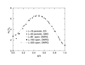
Figure 3: Single magnon line of the $S=1$ Heisenberg AFM from exact diagonalization, quantum Monte Carlo and DMRG for various system sizes and boundary conditions. From Kuhn99 .

The intuition that excitation continua are badly approximated by a sum over some $O(10^{2})$ effective excited states is further corroborated by considering the spectral weight function $S^{+}(q=\pi,\omega)$ [use $A=S^{+}$ in Eq. (4)] for a spin-1/2 Heisenberg antiferromagnet. As shown in Fig. 4, Lanczos vector dynamics roughly catches the right spectral weight, including the $1/\omega$ divergence, as can be seen from the essentially exact correction vector curve, but no convergent behavior can be observed upon an increase of the number of targeted vectors. The very fast Lanczos vector method is thus certainly useful to get a quick overview of spectra, but not suited to detailed quantitative calculations of excitation continua, only excitation bands.

Figure 4: Spectral weight $S^{+}(q=\pi,\omega)$ of the $S=1/2$ Heisenberg AFM from Lanczos vector and correction vector DMRG. $N_{L}$ indicates the number of target states; $M=256$. Note that spectral weight times $\omega$ is shown. From Kuhn99 .

3.2 Correction vector dynamics

Even before the advent of DMRG, another way to obtaining more precise spectral functions had been proposed in Soos89 ; it was first applied using DMRG in Rama97 and Kuhn99 . After preselection of a fixed frequency $\omega$ one may introduce a correction vector

$$|c(\omega+{\rm i}\eta)\rangle=\frac{1}{E_{0}+\omega+{\rm i}\eta-\hat{H}}\hat{A}|0\rangle,$$ (11)

which, if known, allows for trivial calculation of the Green’s function and hence the spectral function at this particular frequency:

$$G_{A}(\omega+{\rm i}\eta)=\langle A|c(\omega+{\rm i}\eta)\rangle.$$ (12)

The correction vector itself is obtained by solving the large sparse linear equation system given by

$$(E_{0}+\omega+{\rm i}\eta-\hat{H})|c(\omega+{\rm i}\eta)\rangle=\hat{A}|0\rangle.$$ (13)

To actually solve this nonhermitean equation system, the current procedure is to split the correction vector into real and imaginary part, to solve the hermitean equation for the imaginary part and exploit the relationship to the real part:

$$[(E_{0}+\omega-\hat{H})^{2}+\eta^{2}]{\rm Im}|c(\omega+{\rm i}\eta)\rangle=-\eta\hat{A}|0\rangle$$ (14)

$${\rm Re}|c(\omega+{\rm i}\eta)\rangle=\frac{\hat{H}-E_{0}-\omega}{\eta}{\rm Im}|c(\omega+{\rm i}\eta)\rangle$$ (15)

The standard method to solve a large sparse linear equation system is the conjugate-gradient method, which effectively generates a Krylov space as does the Lanczos algorithm. The main effor in this method is to provide $\hat{H}^{2}{\rm Im}|c\rangle$. Two remarks are in order. The reduced basis representation of $\hat{H}^{2}$ is obtained by squaring the effective Hamiltonian generated by DMRG. This approximation is found to work extremely well as long as both real and imaginary part of the correction vector are included as target vectors: While the real part is not needed for the evaluation of spectral functions, $(E_{0}+\omega-\hat{H}){\rm Im}|c\rangle\sim{\rm Re}|c\rangle$ due to Eq. (15); and targeting ${\rm Re}|c\rangle$ ensures minimal truncation errors in $\hat{H}{\rm Im}|c\rangle$. The fundamental drawback of using a squared Hamiltonian is that for all iterative eigenvalue or equation solvers the speed of convergence is determined by the matrix condition number which drastically deteriorates by the squaring of a matrix. This might be avoided by using biconjugate or conjugate symmetric equation solvers for Eq. (13) directly.

Alternatively, there is a reformulation of the correction vector method in terms of a minimization principle, which has been called “dynamical DMRG” Jeck02 . While the fundamental approach remains unchanged, the large sparse equation system is replaced by a minimization of the functional

$$W_{A,\eta}(\omega,\psi)=$$ (16)

$$\langle\psi|(E_{0}+\omega-\hat{H})^{2}+\eta^{2}|\psi\rangle+\eta\langle A|\psi\rangle+\eta\langle\psi|A\rangle.$$

At the minimum, the minimizing state is

$$|\psi_{{\rm min}}\rangle={\rm Im}|c(\omega+{\rm i}\eta)\rangle.$$ (17)

Even more importantly, the value of the functional itself is

$$W_{A,\eta}(\omega,\psi)=-\pi\eta C_{A}(\omega+{\rm i}\eta),$$ (18)

such that for the calculation of the spectral function it is not necessary to explicitly use the correction vector. In the simplest form of the correction vector method, the density matrix is formed from targeting four states, $|0\rangle$, $\hat{A}|0\rangle$, ${\rm Im}|c(\omega+{\rm i}\eta)\rangle$ and ${\rm Re}|c(\omega+{\rm i}\eta)\rangle$.

Figure 5: Spectral weight of the $S=1/2$ Heisenberg AFM from correction vector DMRG. $M=256$ states kept. Spectral weights have been calculated for $\omega$-intervals starting from various anchoring frequencies for the correction vector. From Kuhn99 .

As has been shown in Kuhn99 , it is not necessary to calculate a very dense set of correction vectors in $\omega$-space to obtain the spectral function for an entire frequency interval, assuming that the finite convergence factor $\eta$ ensures that an entire range of energies of width $\approx\eta$ is described quite well by the correction vector. It was found that best results are obtained for a two-correction vector approach where two correction vectors are calculated and targeted for two frequencies $\omega_{1}$, $\omega_{2}=\omega_{1}+\Delta\omega$ and the spectral function is obtained for the interval $[\omega_{1},\omega_{2}]$ using the Lanczos method for the approximate Hamiltonian produced by this targeting scheme. This method is, for example, able to provide a high precision result for the spinon continuum in the $S=1/2$ Heisenberg chain where standard Lanczos dynamics fails (Fig. 4).

4 Early attempts at time-evolution

Even though the methods described in the previous section provide high-quality linear-response quantities, they fail in truly out-of-equilibrium situations or for time-dependent Hamiltonians; where they work, they are very time-consuming. It has therefore been of high interest to find DMRG approaches dealing with state evolution in real-time.

To see the advantages of such an approach, consider the following. Essentially all physical quantities of interest involving time can be reduced to the calculation of either equal-time $n$-point correlators such as the (1-point) density

$$\langle n_{i}(t)\rangle=\langle\psi(t)|n_{i}|\psi(t)\rangle=\langle\psi|e^{{\rm i}\hat{H}t}n_{i}e^{-{\rm i}\hat{H}t}|\psi\rangle$$ (19)

or unequal-time $n$-point correlators such as the (2-point) real-time Green’s function

$$G_{ij}(t)=\langle\psi|c^{\dagger}_{i}(t)c_{j}(0)|\psi\rangle=\langle\psi|e^{+{\rm i}\hat{H}t}c_{i}^{\dagger}e^{-{\rm i}\hat{H}t}c_{j}|\psi\rangle.$$ (20)

This expression can be cast in a form very close to Eq. (19) by introducing $|\phi\rangle=c_{j}|\psi\rangle$ such that the desired correlator is then simply given as an equal-time matrix element between two time-evolved states,

$$G_{ij}(t)=\langle\psi(t)|c_{i}^{\dagger}|\phi(t)\rangle.$$ (21)

If both $|\psi(t)\rangle$ and $|\phi(t)\rangle$ can be calculated, a very appealing feature of this approach is that $G_{ij}(t)$ can be evaluated in a single calculation for all $i$ and $t$ as time proceeds. Frequency-momentum space is then reached by a double Fourier transformation. Obviously, finite system-sizes and edge effects as well as algorithmic constraints will impose physical constraints on the largest times and distances $|i-j|$ or minimal frequency and wave vectors resolutions accessible. Nevertheless, this approach might emerge as a very attractive alternative to the current very time-consuming calculations of $G(k,\omega)$ using the dynamical DMRGKuhn99 ; Jeck02 .

The fundamental difficulty of obtaining the above correlators becomes obvious if we examine the time-evolution of the quantum state $|\psi(t=0)\rangle$ under the action of some (for simplicity) time-independent Hamiltonian $\hat{H}|\psi_{n}\rangle=E_{n}|\psi_{n}\rangle$. If the eigenstates $|\psi_{n}\rangle$ are known, expanding $|\psi(t=0)\rangle=\sum_{n}c_{n}|\psi_{n}\rangle$ leads to the well-known time evolution

$$|\psi(t)\rangle=\sum_{n}c_{n}\exp(-{\rm i}E_{n}t)|\psi_{n}\rangle,$$ (22)

where the modulus of the expansion coefficients of $|\psi(t)\rangle$ is time-independent. A sensible Hilbert space truncation is given by a projection onto the large-modulus eigenstates. In strongly correlated systems, however, we usually have no good knowledge of the eigenstates. Instead, one uses some orthonormal basis with unknown eigenbasis expansion, $|k\rangle=\sum_{n}a_{kn}|\psi_{n}\rangle$. The time evolution of the state $|\psi(t=0)\rangle=\sum_{k}d_{k}(0)|k\rangle$ then reads

$$|\psi(t)\rangle=\sum_{k}\left(\sum_{n}d_{k}(0)a_{kn}e^{-{\rm i}E_{n}t}\right)|k\rangle\equiv\sum_{k}d_{k}(t)|k\rangle,$$ (23)

where the modulus of the expansion coefficients $d_{k}(t)$ is time-dependent. For a general orthonormal basis, Hilbert space truncation at one fixed time (i.e. $t=0$) will therefore not ensure a reliable approximation of the time evolution. Also, energy differences matter in time evolution due to the phase factors $e^{-{\rm i}(E_{n}-E_{n^{\prime}})t}$ in $|d_{k}(t)|^{2}$. Thus, a good approximation to the low-energy Hamiltonian alone (as provided by DMRG) is of limited use.

Static time-dependent DMRG. Cazalilla and MarstonCaza02 were the first to exploit DMRG to systematically calculate time-dependent quantum many-body effects. They studied a time-dependent Hamiltonian $\hat{H}(t)\equiv\hat{H}(0)+\hat{V}(t)$, where $\hat{V}(t)$ encodes the time-dependent part of the Hamiltonian. After applying a standard DMRG calculation to the Hamiltonian $\hat{H}(t=0)$, the time-dependent Schrödinger equation was numerically integrated forward in time. The effective Hamiltonian in the reduced Hilbert space was built as $\hat{H}_{{\rm eff}}(t)=\hat{H}_{{\rm eff}}(0)+\hat{V}_{{\rm eff}}(t)$, where $\hat{H}_{{\rm eff}}(0)$ was taken as the last superblock Hamiltonian approximating $\hat{H}(0)$. $\hat{V}_{{\rm eff}}(t)$ as an approximation to $\hat{V}$ was built using the representations of operators in the final block bases. The initial condition was obviously to take $|\psi(0)\rangle$ as the ground state obtained by the preliminary DMRG run. This procedure amounts to working within a static reduced Hilbert space, namely that optimal at $t=0$, and projecting all wave functions and operators onto it.

In this approach the hope is that an effective Hamiltonian obtained by targeting the ground state of the $t=0$ Hamiltonian is capable to catch the states that will be visited by the time-dependent Hamiltonian during time evolution. This approach must however break down after relatively short times as the full Hilbert space is explored, as became quickly obvious.

Dynamic time-dependent DMRG. Several attempts have been made to improve on static time-dependent DMRG by enlarging the reduced Hilbert space using information on the time-evolution, such that the time-evolving state has large support on that dynamic Hilbert space for longer times. Whatever procedure for enlargement is used, the problem remains that the number of DMRG states $m$ grows with the desired simulation time as they have to encode more and more different physical states. As calculation time scales as $m^{3}$, this type of approach will meet its limitations somewhat later in time.

All enlargement procedures rest on the ability of DMRG to describe – at some numerical expense – small sets of states (“target states”) very well instead of just one.

The simplest approach is to target the set $\{|\psi_{i}\rangle\}=\{|\psi(0)\rangle,\hat{H}|\psi(0)\rangle,\hat{H}^{2}|\psi(0)\rangle,\ldots\}$. Alternatively, one might consider the Krylov vectors formed from this set. Results improve, but not decisively.

A much more time-consuming, but also much better performing approach has been demonstrated by Luo, Xiang and Wang Luo03 . They use a density matrix that is given by a superposition of states $|\psi(t_{i})\rangle$ at various times of the evolution, $\hat{\rho}=\sum_{i=0}^{N_{t}}\alpha_{i}|\psi(t_{i})\rangle\langle\psi(t_{i})|$ with $\sum\alpha_{i}=1$ for the determination of the reduced Hilbert space. Of course, these states are not known initially; it was proposed by them to start within the framework of infinite-system DMRG from a small DMRG system and evolve it in time. For a very small system this procedure is exact. For this system size, the state vectors $|\psi(t_{i})\rangle$ are used to form the density matrix. This density matrix then determines the reduced Hilbert space for the next larger system, taking into account how time-evolution explores the Hilbert space for the smaller system. One then moves on to the next larger DMRG system where the procedure is repeated. This is of course very time-consuming.

SchmitteckertSchm04 has computed the transport through a small interacting nanostructure using an Hilbert space enlarging approach, based on the time evolution operator. To this end, he splits the problem into two parts: By obtaining a relatively large number of low-lying eigenstates exactly (within time-independent DMRG precision), one can calculate their time evolution exactly. For the subspace orthogonal to these eigenstates, he implements the matrix exponential $|\psi(t+\Delta t)\rangle=\exp(-{\rm i}\hat{H}\Delta t)|\psi(t)\rangle$ using the Krylov subspace approximation. For any block-site configuration during sweeping, he evolves the state in time, obtaining $|\psi(t_{i})\rangle$ at fixed times $t_{i}$. These are targeted in the density matrix, such that upon sweeping forth and back a Hilbert space suitable to describe all of them at good precision should be obtained. For numerical efficiency, he carries out this procedure to convergence for some small time, which is then increased upon sweeping, bringing more and more states $|\psi(t_{i})\rangle$ into the density matrix. Again, this is a very time-consuming approach.

5 Time-evolving block decimation

Decisive progress came from an unexpected corner, namely quantum information theory, when Vidal proposed an algorithm for simulating quantum time evolutions of one-dimensional systems efficiently on a classical computer Vida04 ; Vida03a . His algorithm, known as TEBD [time-evolving block decimation] algorithm, is based on matrix product statesFann92 ; Klum93 ; as it turned out, it is so closely linked to DMRG concepts, that his ideas could be implemented easily into DMRG, leading to an adaptive time-dependent DMRG, where the DMRG state space adapts itself in time to the time-evolving quantum state. In this section, we will explain his algorithm.

A useful concept is that of a Schmidt decomposition: Consider a quantum state $|\psi\rangle=\sum_{ij}\psi_{ij}|i\rangle\otimes|j\rangle$ as introduced before, with $N^{S}$ states $|i\rangle$ and $N^{E}$ states $|j\rangle$. Assuming without loss of generality $N^{S}\geq N^{E}$, we form the $(N^{S}\times N^{E})$-dimensional matrix $A$ with $A_{ij}=\psi_{ij}$. Singular value decomposition guarantees $A=UDV^{T}$, where $U$ is $(N^{S}\times N^{E})$-dimensional with orthonormal columns, $D$ is a $(N^{E}\times N^{E})$-dimensional diagonal matrix with non-negative entries $D_{\alpha\alpha}=\sqrt{w_{\alpha}}$, and $V^{T}$ is a $(N^{E}\times N^{E})$-dimensional unitary matrix; $|\psi\rangle$ can be written as

$$|\psi\rangle = \sum_{i=1}^{N^{S}}\sum_{\alpha=1}^{N^{E}}\sum_{j=1}^{N^{E}}U_{i\alpha}\sqrt{w_{\alpha}}V^{T}_{\alpha j}|i\rangle|j\rangle$$

$$= \sum_{\alpha=1}^{N^{E}}\sqrt{w_{\alpha}}\left(\sum_{i=1}^{N^{S}}U_{i\alpha}|i\rangle\right)\left(\sum_{j=1}^{N^{E}}V_{j\alpha}|j\rangle\right).$$

The orthonormality properties of $U$ and $V^{T}$ ensure that $|w_{\alpha}^{S}\rangle=\sum_{i}U_{i\alpha}|i\rangle$ and $|w_{\alpha}^{E}\rangle=\sum_{j}V_{j\alpha}|j\rangle$ form orthonormal bases of system and environment respectively, in which the Schmidt decomposition

$$|\psi\rangle=\sum_{\alpha=1}^{N_{{\rm Schmidt}}}\sqrt{w_{\alpha}}|w_{\alpha}^{S}\rangle|w_{\alpha}^{E}\rangle$$ (25)

holds. $N^{S}N^{E}$ coefficients $\psi_{ij}$ are reduced to $N_{{\rm Schmidt}}\leq N^{E}$ non-zero coefficients $\sqrt{w_{\alpha}}$, $w_{1}\geq w_{2}\geq w_{3}\geq\ldots$. Relaxing the assumption $N^{S}\geq N^{E}$, one has

$$N_{{\rm Schmidt}}\leq\min(N^{S},N^{E}).$$ (26)

Upon tracing out environment or system the reduced density matrices for system and environment are found to be

$$\hat{\rho}_{S}=\sum_{\alpha}^{N_{{\rm Schmidt}}}w_{\alpha}|w_{\alpha}^{S}\rangle\langle w_{\alpha}^{S}|;\quad\hat{\rho}_{E}=\sum_{\alpha}^{N_{{\rm Schmidt}}}w_{\alpha}|w_{\alpha}^{E}\rangle\langle w_{\alpha}^{E}|.$$ (27)

DMRG reduced density matrix analysis and the Schmidt decomposition therefore yield exactly the same information. This fact was understood from the very beginning of DMRG, although we had not heard the term “Schmidt decomposition”. In fact, the singular value decomposition representation of the wavefunction was understood before the density matrix representation.

Let us now formulate the TEBD simulation algorithm. In the original exposition of the algorithm Vida03a , one starts from a representation of a quantum state $|\psi\rangle=\sum_{\sigma_{1}\ldots\sigma_{L}}\psi_{\sigma_{1},\ldots,\sigma_{L}}|\sigma_{1}\ldots\sigma_{L}\rangle$ where the coefficients for the states are decomposed as a product of tensors,

$$\psi_{\sigma_{1},\ldots,\sigma_{L}}=\sum_{\alpha_{1},\ldots,\alpha_{L-1}}\Gamma^{1}_{\alpha_{1}}[\sigma_{1}]\lambda^{1}_{\alpha_{1}}\Gamma^{2}_{\alpha_{1}\alpha_{2}}[\sigma_{2}]\lambda^{2}_{\alpha_{2}}\Gamma^{3}_{\alpha_{2}\alpha_{3}}[\sigma_{3}]\cdots\Gamma^{L}_{\alpha_{L-1}}[\sigma_{L}].$$ (28)

It is of no immediate concern to us how the $\Gamma$ and $\lambda$ tensors are constructed explicitly for a given physical situation. Let us assume that they have been determined such that they approximate the true wave function close to the optimum obtainable within the class of wave functions having such coefficients; this is indeed possible as will be discussed below. There are, in fact, two ways of doing it: within the framework of DMRG, or by a continuous imaginary time evolution from some simple product state, as discussed in Ref. Vida04 .

The ansatz can be visualized: the (diagonal) tensors $\lambda^{i}$, $i=1,\ldots,L-1$ are associated with the bonds $i$, whereas $\Gamma^{i}$, $i=2,\ldots,L-1$ links (transfers) from bond $i$ to bond $i-1$ across site $i$. Note that at the boundaries ($i=1,L$) the structure of the $\Gamma$ is modified. The sums run over $m$ states $|\alpha_{i}\rangle$ living in auxiliary state spaces on bond $i$. A priori, these states have no physical meaning.

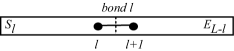
Figure 6: Bipartitioning by cutting bond $l$ between sites $l$ and $l+1$.

The $\Gamma$ and $\lambda$ tensors are constructed such that for an arbitrary cut of the system into a part $S_{l}$ of length $l$ and a part $E_{L-l}$ of length $L-l$ at bond $l$, the Schmidt decomposition for this bipartite splitting reads

$$|\psi\rangle=\sum_{\alpha_{l}}\lambda^{l}_{\alpha_{l}}|w_{\alpha_{l}}^{S_{l}}\rangle|w_{\alpha_{l}}^{E_{L-l}}\rangle,$$ (29)

with

$$|w_{\alpha_{l}}^{S_{l}}\rangle=\sum_{\alpha_{1},\ldots,\alpha_{l-1}}\sum_{\sigma_{1},\ldots,\sigma_{l}}\Gamma^{1}_{\alpha_{1}}[\sigma_{1}]\lambda^{1}_{\alpha_{1}}\cdots\Gamma^{l}_{\alpha_{l-1}\alpha_{l}}[\sigma_{l}]|\sigma_{1}\rangle\otimes\cdots\otimes|\sigma_{l}\rangle,$$ (30)

and

$$|w_{\alpha_{l}}^{E_{L-l}}\rangle = \sum_{\alpha_{l},\ldots,\alpha_{L-1}}\sum_{\sigma_{l+1},\ldots,\sigma_{L}}\Gamma^{l+1}_{\alpha_{l}\alpha_{l+1}}[\sigma_{l+1}]\lambda^{l+1}_{\alpha_{l+1}}\cdots\Gamma^{L}_{\alpha_{L-1}}[\sigma_{L}]\times$$ (31)

$$|\sigma_{l+1}\rangle\otimes\cdots\otimes|\sigma_{L}\rangle,$$

where $|\psi\rangle$ is normalized and the sets of $\{|w_{\alpha_{l}}^{S_{l}}\rangle\}$ and $\{|w_{\alpha_{l}}^{E_{L-l}}\rangle\}$ are orthonormal. This implies, for example, that

$$\sum_{\alpha_{l}}(\lambda_{\alpha_{l}}^{l})^{2}=1.$$ (32)

We can see that (leaving aside normalization considerations for the moment, see Dale04 ) this representation may be expressed as a matrix product state if we choose for $A^{i}[\sigma_{i}]=\sum_{\alpha,\beta}A^{i}_{\alpha\beta}[\sigma_{i}]|\alpha\rangle\langle\beta|$

$$A_{\alpha\beta}^{i}[\sigma_{i}]=\Gamma^{i}_{\alpha\beta}[\sigma_{i}]\lambda^{i}_{\beta},$$ (33)

except for $i=1$, and $i=L$, where expressions are slightly modified.

Let us now consider the time evolution for a typical (possibly time-dependent) Hamiltonian with nearest-neighbor interactions:

$$\hat{H}=\sum_{i\>\rm odd}\hat{F}_{i,i+1}+\sum_{j\rm\>even}\hat{G}_{j,j+1},$$ (34)

$\hat{F}_{i,i+1}$ and $\hat{G}_{j,j+1}$ are the local Hamiltonians on the odd bonds linking $i$ and $i+1$, and the even bonds linking $j$ and $j+1$. While all $\hat{F}$ and $\hat{G}$ terms commute among each other, $\hat{F}$ and $\hat{G}$ terms do in general not commute if they share one site. Then the time evolution operator may be approximately represented by a (first order) Trotter expansion as

$${\rm e}^{-{\rm i}\hat{H}\delta t}=\prod_{i\rm\>odd}{\rm e}^{-{\rm i}\hat{F}_{i,i+1}\delta t}\prod_{j\rm\>even}{\rm e}^{-{\rm i}\hat{G}_{j,j+1}\delta t}+\mathcal{O}(\delta t^{2}),$$ (35)

and the time evolution of the state can be computed by repeated application of the two-site time evolution operators $\exp({-{\rm i}\hat{G}_{j,j+1}\delta t})$ and $\exp({-{\rm i}\hat{F}_{i,i+1}\delta t})$. This is a well-known procedure in particular in Quantum Monte CarloSuzu76 where it serves to carry out imaginary time evolutions (e.g. checkerboard decomposition).

The TEBD simulation algorithm now runs as followsVida04 ; Vida03a :

1. Perform the following two steps for all even bonds (the order does not matter):

   • Apply $\exp({-{\rm i}\hat{G}_{l,l+1}\delta t})$ to $|\psi(t)\rangle$. For each local time update, a new wave function is obtained. The number of degrees of freedom on the “active” bond thereby increases, as will be detailed below.

   • Carry out a Schmidt decomposition cutting this bond and retain as in DMRG only those $m$ degrees of freedom with the highest weight in the decomposition.

2. Repeat this two-step procedure for all odd bonds, applying $\exp({-{\rm i}\hat{F}_{l,l+1}\delta t})$.

3. This completes one Trotter time step. One may now evaluate expectation values at selected time steps, and continues the algorithm from step 1.

Let us now consider some computational details.
(i) Consider a local time evolution operator acting on bond $l$, i.e. sites $l$ and $l+1$, for a state $|\psi\rangle$. The Schmidt decomposition of $|\psi\rangle$ after partitioning by cutting bond $l$ reads

$$|\psi\rangle=\sum_{\alpha_{l}=1}^{M}\lambda^{l}_{\alpha_{l}}|w_{\alpha_{l}}^{S_{l}}\rangle|w_{\alpha_{l}}^{E_{L-l}}\rangle.$$ (36)

Using Eqs. (30) and (31), we find after expanding $|w_{\alpha_{l}}^{S_{l}}\rangle$ into $|w_{\alpha_{l-1}}^{S_{l-1}}\rangle$ and $|\sigma_{l}\rangle$, and similarly for $|w_{\alpha_{l}}^{E_{L-l}}\rangle$,

$$|\psi\rangle = \sum_{\alpha_{l-1}\alpha_{l}\alpha_{l+1}}\sum_{\sigma_{l}\sigma_{l+1}}\lambda^{l-1}_{\alpha_{l-1}}\Gamma^{l}_{\alpha_{l-1}\alpha_{l}}[\sigma_{l}]\lambda^{l}_{\alpha_{l}}\Gamma^{l+1}_{\alpha_{l}\alpha_{l+1}}[\sigma_{l+1}]\lambda^{l+1}_{\alpha_{l+1}}\times$$ (37)

$$|w_{\alpha_{l-1}}^{S_{l-1}}\rangle|\sigma_{l}\rangle|\sigma_{l+1}\rangle|w_{\alpha_{l+1}}^{E_{L-(l+1)}}\rangle.$$

We note, that this has the form of a typical DMRG state for two blocks and two sites

$$|\psi\rangle=\sum_{m_{l-1}}\sum_{\sigma_{l}}\sum_{\sigma_{l+1}}\sum_{m_{l+1}}\psi_{m_{l-1}\sigma_{l}\sigma_{l+1}m_{l+1}}|w^{S}_{m_{l-1}}\rangle|\sigma_{l}\rangle|\sigma_{l+1}\rangle|w^{E}_{m_{l+1}}\rangle.$$ (38)

The local time evolution operator on site $l,l+1$ can be expanded as

$$\hat{U}_{l,l+1}=\sum_{\sigma_{l}\sigma_{l+1}}\sum_{\sigma_{l}^{\prime}\sigma_{l+1}^{\prime}}U^{\sigma_{l}^{\prime}\sigma_{l+1}^{\prime}}_{\sigma_{l}\sigma_{l+1}}|\sigma_{l}^{\prime}\sigma_{l+1}^{\prime}\rangle\langle\sigma_{l}\sigma_{l+1}|$$ (39)

and generates $|\psi^{\prime}\rangle=\hat{U}_{l,l+1}|\psi\rangle$.

$$|\psi^{\prime}\rangle=\sum_{\alpha_{l-1}\alpha_{l+1}}\sum_{\sigma_{l}\sigma_{l+1}}\Theta^{\sigma_{l}\sigma_{l+1}}_{\alpha_{l-1}\alpha_{l+1}}|w_{\alpha_{l-1}}^{S_{l-1}}\rangle|\sigma_{l}\rangle|\sigma_{l+1}\rangle|w_{\alpha_{l+1}}^{E_{L-(l+1)}}\rangle,$$ (40)

where

$$\Theta^{\sigma_{l}\sigma_{l+1}}_{\alpha_{l-1}\alpha_{l+1}}=\lambda^{l-1}_{\alpha_{l-1}}\sum_{\alpha_{l}\sigma_{l}^{\prime}\sigma_{l+1}^{\prime}}\Gamma^{l}_{\alpha_{l-1}\alpha_{l}}[\sigma_{l}^{\prime}]\lambda^{l}_{\alpha_{l}}\Gamma^{l+1}_{\alpha_{l}\alpha_{l+1}}[\sigma_{l+1}^{\prime}]\lambda^{l+1}_{\alpha_{l+1}}U^{\sigma_{l}\sigma_{l+1}}_{\sigma_{l}^{\prime}\sigma_{l+1}^{\prime}}.$$ (41)

(ii) Now a new Schmidt decomposition identical to that in DMRG can be carried out for $|\psi^{\prime}\rangle$: cutting once again bond $l$, there are now $mn_{{\rm site}}$ states in each part of the system, leading to

$$|\psi^{\prime}\rangle=\sum_{\alpha_{l}=1}^{mn_{{\rm site}}}\tilde{\lambda}^{l}_{\alpha_{l}}|\tilde{w}_{\alpha_{l}}^{S_{l}}\rangle|\tilde{w}_{\alpha_{l}}^{E_{L-l}}\rangle.$$ (42)

In general the states and coefficients of the decomposition will have changed compared to the decomposition (36) previous to the time evolution, and hence they are adaptive. We indicate this by introducing a tilde for these states and coefficients. As in DMRG, if there are more than $m$ non-zero eigenvalues, we now choose the $m$ eigenvectors corresponding to the largest $\tilde{\lambda}^{l}_{\alpha_{l}}$ to use in these expressions. The error in the final state produced as a result is proportional to the sum of the magnitudes of the discarded eigenvalues. After normalization, to allow for the discarded weight, the state reads

$$|\psi^{\prime}\rangle=\sum_{\alpha_{l}=1}^{m}\lambda^{l}_{\alpha_{l}}|w_{\alpha_{l}}^{S_{l}}\rangle|w_{\alpha_{l}}^{E_{L-l}}\rangle.$$ (43)

Note again that the states and coefficients in this superposition are in general different from those in Eq. (36); we have now dropped the tildes again, as this superposition will be the starting point for the next time evolution (state adaption) step.

The key point about the TEBD simulation algorithm is that a DMRG-style truncation to keep the most relevant density matrix eigenstates (or the maximum amount of entanglement) is carried out at each time step. This is in contrast to previous time-dependent DMRG methods, where the basis states were chosen before the time evolution, and did not “adapt” to optimally represent the state at each instant of time.

6 Adaptive time-dependent DMRG

DMRG generates position-dependent $m\times m$ matrix-product states as block states for a reduced Hilbert space of $m$ states; the auxiliary state space to a bond is given by the Hilbert space of the block at whose end the bond sits. This physical meaning attached to the auxiliary state spaces implies that they carry good quantum numbers for all block sizes. The big advantage is that using good quantum numbers allows us to exclude a large amount of wave function coefficients as being 0, drastically speeding up all calculations by at least one, and often two orders of magnitude.

The effect of the finite-system DMRG algorithmWhit93 is now to shift the two free sites through the chain, growing and shrinking the blocks S and E as illustrated in Fig. 7. At each step, the ground state is redetermined and a new Schmidt decomposition carried out in which the system is cut between the two free sites, leading to a new truncation and new reduced basis transformations (2 matrices $A$ adjacent to this bond).

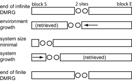
Figure 7: Finite-system DMRG algorithm. Block growth and shrinkage. For the adaptive time-dependent DMRG, replace ground state optimization by local time evolution.

As the actual decomposition and truncation procedure in DMRG and the TEBD simulation algorithm are identical, one can use the finite-system algorithm to carry out the sequence of local time evolutions (instead of, or after, optimizing the ground state), thus constructing by Schmidt decomposition and truncation new block states best adapted to a state at any given point in the time evolution (hence adaptive block states) as in the TEBD algorithm, while maintaining the computational efficiency of DMRG. To do this, one needs not only all reduced basis transformations, but also the wave function $|\psi\rangle$ in a two-block two-site configuration such that the bond that is currently updated consists of the two free sites. This implies that $|\psi\rangle$ has to be transformed between different configurations. In finite-system DMRG such a transformation, which was first implemented by WhiteWhit96b (“state prediction”) is routinely used to predict the outcome of large sparse matrix diagonalizations, which no longer occur during time evolution. Here, it merely serves as a basis transformation.

The adaptive time-dependent DMRG algorithm which incorporates the TEBD simulation algorithm in the DMRG framework is therefore set up as follows:

• Set up a conventional finite-system DMRG algorithm with state prediction using the Hamiltonian at time $t=0$, $\hat{H}(0)$, to determine the ground state of some system of length $L$ using effective block Hilbert spaces of dimension $M$. At the end of this stage of the algorithm, we have for blocks of all sizes $l$ reduced orthonormal bases spanned by states $|m_{l}\rangle$, which are characterized by good quantum numbers. Also, we have all reduced basis transformations, corresponding to the matrices $A$.

• For each Trotter time step, use the finite-system DMRG algorithm to run one sweep with the following modifications:

  • For each even bond apply the local time evolution $\hat{U}$ at the bond formed by the free sites to $|\psi\rangle$. This is a very fast operation compared to determining the ground state, which is usually done instead in the finite-system algorithm.

  • As always, perform a DMRG truncation at each step of the finite-system algorithm, hence $O(L)$ times.

  • Use White’s prediction method to shift the free sites by one.

• In the reverse direction, apply step (i) to all odd bonds.

• As in standard finite-system DMRG evaluate operators when desired at the end of some time steps. Note that there is no need to generate these operators at all those time steps where no operator evaluation is desired, which will, due to the small Trotter time step, be the overwhelming majority of steps.

Note that one can also perform every bond evolution operator at each half-sweep, in order. This does not worsen the Trotter error, since in the reverse sweep the operators are applied in reverse order.

The calculation time of adaptive time-dependent DMRG scales linearly in $L$, as opposed to the static time-dependent DMRG which does not depend on $L$. The diagonalization of the density matrices (Schmidt decomposition) scales as $n_{{\rm site}}^{3}m^{3}$; the preparation of the local time evolution operator as $n_{{\rm site}}^{6}$, but this may have to be done only rarely e.g. for discontinuous changes of interaction parameters. Carrying out the local time evolution scales as $n_{{\rm site}}^{4}m^{2}$; the basis transformation scales as $n_{{\rm site}}^{2}m^{3}$. As $m\gg n_{{\rm site}}$ typically, the algorithm is of order $O(Ln_{{\rm site}}^{3}m^{3})$ at each time step.

The performance of this method has been tested in various applications in the context of ultracold atom physics Dale04 ; Koll04 ; Koll05 ; Treb05 , but also for far-from-equilibrium dynamics Gobe04 and for spectral functions Whit04 ; some of these applications will serve as examples in the following.

7 Far-from-equilibrium dynamics

In this section, we consider the dynamics of a system far from equilbrium using adaptive time-dependent DMRGGobe04 . The following example, for which an exact solution is available, shows that time-dependent DMRG can also perform in situations where dynamical DMRG must surely fail.

The initial state $|\mathrm{ini}\rangle=|\uparrow\dots\uparrow\downarrow\dots\downarrow\rangle$ on the one-dimensional spin-$1/2$ chains is subjected to the dynamics of the Heisenberg model

$$H=\sum_{n}S^{x}_{n}S^{x}_{n+1}+S^{y}_{n}S^{y}_{n+1}+J_{z}S^{z}_{n}S^{z}_{n+1}\equiv\sum_{n}h_{n}.$$ (44)

We set $\hbar=1$, defining time to be 1/energy with the energy unit chosen as the $J_{xy}$ interaction.

Often it is useful to map the Heisenberg model onto a model of interacting spinless fermions with nearest-neighbour hopping:

$$H = \sum_{n}\left[\frac{1}{2}(c_{n}^{\dagger}c_{n+1}^{\phantom{\dagger}}+c_{n+1}^{\dagger}c_{n}^{\phantom{\dagger}})\right.$$ (45)

$$\left.+J_{z}(c^{\dagger}_{n}c_{n}^{\phantom{\dagger}}-\frac{1}{2})(c^{\dagger}_{n+1}c^{\phantom{\dagger}}_{n+1}-\frac{1}{2})\right].$$

In particular, the case $J_{z}=0$ describes free fermions on a lattice, and can be solved exactly. In the following we will focus on this case. Note that in that case the initial state with two large ferromagnetic domains separated by a domain wall in the center is a highly excited state; the ground state exhibits power-law decaying antiferromagnetic correlations.

The time evolution delocalizes the domain wall over the entire chain; the magnetization profile for the initial state $|\mathrm{ini}\rangle$ reads Anta99 :

$$S_{z}(n,t)=\langle\psi(t)|S_{n}^{z}|\psi(t)\rangle=-1/2\sum_{j=1-n}^{n-1}J_{j}^{2}(t),$$ (46)

where $J_{j}$ is the Bessel function of the first kind. $n=\ldots,-3,-2,-1,0,1,2,3,\ldots$ labels chain sites with the convention that the first site in the right half of the chain has label $n=1$. As the total energy of the system is conserved, the state cannot relax to the ground state. The exact solution reveals a nontrivial behaviour with a complicated substructure in the magnetization profile, which is a good benchmark for DMRG.

Possible errors. Two main sources of error occur in the adaptive t-DMRG:
(i) The Trotter error due to the Trotter decomposition. For an $n$th-order Trotter decomposition Suzu76 , the error made in one time step $dt$ is of order $Ldt^{n+1}$. To reach a given time $t$ one has to perform $t/dt$ time-steps, such that in the worst case the error grows linearly in time $t$ and the resulting error is of order $L(dt)^{n}t$.
(ii) The DMRG truncation error due to the representation of the time-evolving quantum state in reduced (albeit “optimally” chosen) Hilbert spaces and to the repeated transformations between different truncated basis sets. While the truncation error $\epsilon$ that sets the scale of the error of the wave function and operators is typically very small, here it will strongly accumulate as $O(Lt/dt)$ truncations are carried out up to time $t$. This is because the truncated DMRG wave function has norm less than one and is renormalized at each truncation by a factor of $(1-\epsilon)^{-1}>1$. Truncation errors should therefore accumulate roughly exponentially with an exponent of $\epsilon Lt/dt$, such that eventually the adaptive t-DMRG will break down at too long times. The accumulated truncation error should decrease considerably with an increasing number of kept DMRG states $m$. For a fixed time $t$, it should decrease as the Trotter time step $dt$ is increased, as the number of truncations decreases with the number of time steps $t/dt$.

At this point, it is worthwhile to mention that our subsequent error analysis should also be pertinent to the very closely related time-evolution algorithm introduced by Verstraete et al.Vers04a , which also involves both Trotter and truncation errors.

We remind the reader that no error is encountered in the application of the local time evolution operator $U_{n}$ to the state $|\psi\rangle$.

Error analysis. We use two main measures for the error:
(i) As a measure for the overall error we consider the magnetization deviation, the maximum deviation of the local magnetization found by DMRG from the exact result,

$$\mathrm{err}(t)=\mathrm{max}_{n}|\langle S^{z}_{n,\mathrm{DMRG}}(t)\rangle-\langle S^{z}_{n,\mathrm{exact}}(t)\rangle|.$$ (47)

(ii) As a measure which excludes the Trotter error we use the forth-back deviation $FB(t)$, which we define as the deviation between the initial state $|\mathrm{ini}\rangle$ and the state $|fb(t)\rangle=U(-t)U(t)|\mathrm{ini}\rangle$, i.e. the state obtained by evolving $|\mathrm{ini}\rangle$ to some time $t$ and then back to $t=0$ again. If we Trotter-decompose the time evolution operator $U(-t)$ into odd and even bonds in the reverse order of the decomposition of $U(t)$, the identity $U(-t)=U(t)^{-1}$ holds without any Trotter error, and the forth-back deviation has the appealing property to capture the truncation error only.

As the DMRG setup used in this particular calculation did not allow easy access to the fidelity $|\langle\mathrm{ini}|fb(t)\rangle|$ (a calculation which is not a problem in principle, see Treb05 ), the forth-back deviation was defined to be the $L_{2}$ measure for the difference of the magnetization profiles of $|\mathrm{ini}\rangle$ and $|fb(t)\rangle$,

$$FB(t)=\left(\sum_{n}\left(\langle\mathrm{ini}|S^{z}_{n}|\mathrm{ini}\rangle-\langle fb(t)|S^{z}_{n}|fb(t)\rangle\right)^{2}\right)^{1/2}\!\!\!\!\!\!\!.$$ (48)

In order to control Trotter and truncation error, two DMRG control parameters are available, the number of DMRG states $m$ and the Trotter time step $dt$.

Figure 8: Magnetization deviation ${\rm err}(t)$ as a function of time for different numbers $m$ of DMRG states. The Trotter time interval is fixed at $dt=0.05$. Again, two regimes can be distinguished: For early times, for which the Trotter error dominates, the error is slowly growing (essentially linearly) and independent of $m$ (regime A); for later times, the error is entirely given by the truncation error, which is $m$-dependent and growing fast (almost exponential up to some saturation; regime B). The transition between the two regimes occurs at a well-defined “runaway time” $t_{R}$ (small squares). The inset shows a monotonic, roughly linear dependence of $t_{R}$ on $m$. From Gobe04 .

The dependence on $dt$ is twofold: on the one hand, decreasing $dt$ reduces the Trotter error by some power of $dt^{n}$ exactly as in QMC; on the other hand, the number of truncations increases, such that the truncation error is enhanced. It is therefore not a good strategy to choose $dt$ as small as possible. The truncation error can however be decreased by increasing $m$.

Consider the dependence of the magnetization deviation $\mathrm{err}(t)$ on the number $m$ of DMRG states. In Fig. 8, $\mathrm{err}(t)$ is plotted for a fixed Trotter time step $dt=0.05$ and different values of $m$. One sees that a $m$-dependent “runaway time” $t_{R}$ separates two regimes: for $t<t_{R}$ (regime A), the deviation grows essentially linearly in time and is independent of $m$, for $t>t_{R}$ (regime B), it suddenly starts to grow more rapidly than any power-law as expected of the truncation error. In the inset of Fig. 8, $t_{R}$ is seen to increase roughly linearly with growing $m$. As $m\rightarrow\infty$ corresponds to the complete absence of the truncation error, the $m$-independent bottom curve of Fig. 8 is a measure for the deviation due to the Trotter error alone and the runaway time can be read off very precisely as the moment in time when the truncation error starts to dominate.

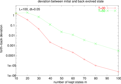
Figure 9: The forth-back error $FB(t)$ for $t=50$ and $t=30$, as function of $m$. Here, $L=100$, $dt=0.05$. From Gobe04 .

That the crossover from a dominating Trotter error at short times and a dominating truncation error at long times is so sharp may seem surprising at first, but can be explained easily by observing that the Trotter error grows only linearly in time, but the accumulated truncation error grows almost exponentially in time.

To see that nothing special is happening at $t_{R}$, consider also Fig. 9, where the Trotter-error free $FB(t)$ is plotted as a function of $m$, for $t=30$ and $t=50$. An approximately exponential increase of the accuracy of the method with growing $m$ is observed for a fixed time. Our numerical results that indicate a roughly linear time-dependence of $t_{R}$ on $m$ (inset of Fig. 8) are the consequence of some balancing of very fast growth of precision with $m$ and decay of precision with $t$.

The runaway time thus indicates an imminent breakdown of the method and is a good, albeit very conservative measure of available simulation times. We expect the above error analysis for the adaptive t-DMRG to be generic for other models. The truncation error will remain also in approaches that dispose of the Trotter error; maximally reachable simulation times should therefore be roughly the similar. Even if for high precision calculation the Trotter error may dominate for a long time, in the long run it is always the truncation error that causes the breakdown of the method at some point in time.

8 Finite temperature

After the previous discussion on the difficulties of simulating the time-evolution of pure states in subsets of large Hilbert spaces it may seem that the time-evolution of mixed states (density matrices) is completely out of reach. It is however easy to see that a thermal density matrix $\hat{\rho}_{\beta}\equiv\exp[-\beta\hat{H}]$ can be constructed as a pure state in an enlarged Hilbert space and that Hamiltonian dynamics of the density matrix can be calculated considering just this pure state (dissipative dynamics being more complicated). In the DMRG context, this has first been pointed out by Verstraete, Garcia-Rípoll and CiracVers04a and Zwolak and VidalZwol04 , using essentially information-theoretical language; it has also been used previously in pure statistical physics language in e.g. high-temperature series expansionsBuhl00 .

To this end, consider the completely mixed state $\hat{\rho}_{0}\equiv 1$. Let us assume that the dimension of the local physical state space $\{|\sigma_{i}\rangle\}$ of a physical site is $n$. Introduce now a local auxiliary state space $\{|\tau_{i}\rangle\}$ of the same dimension $n$ on an auxiliary site. The local physical site is thus replaced by a rung of two sites, and a one-dimensional chain by a two-leg ladder of physical and auxiliary sites on top and bottom rungs. Prepare now each rung $i$ in the Bell state

$$|\psi_{0}^{i}\rangle=\frac{1}{\sqrt{n}}\left[\sum_{\sigma_{i}=\tau_{i}}^{n}|\sigma_{i}\tau_{i}\rangle\right].$$ (49)

Other choices of $|\psi_{0}^{i}\rangle$ are equally feasible, as long as they maintain in their product states maximal entanglement between physical states $|\sigma_{i}\rangle$ and auxiliary states $|\tau_{i}\rangle$. Evaluating now the expectation value of some local operator $\hat{O}_{\sigma}^{i}$ acting on the physical state space with respect to $|\psi_{0}^{i}\rangle$, one finds

$$\langle\psi_{0}^{i}|\hat{O}_{\sigma}^{i}|\psi_{0}^{i}\rangle=\sum_{\sigma_{i}=\tau_{i}}\sum_{\sigma_{i}^{\prime}=\tau_{i}^{\prime}}\frac{1}{n}\left[\langle\sigma_{i}\tau_{i}|\hat{O}_{\sigma}^{i}\otimes 1_{\tau}^{i}|\sigma_{i}^{\prime}\tau_{i}^{\prime}\rangle\right].$$

The double sum collapses to

$$\langle\psi_{0}^{i}|\hat{O}_{\sigma}^{i}|\psi_{0}^{i}\rangle=\frac{1}{n}\sum_{\sigma_{i}=1}^{n}\langle\sigma_{i}|\hat{O}_{\sigma}^{i}|\sigma_{i}\rangle,$$

and we see that the expectation value of $\hat{O}_{\sigma}^{i}$ with respect to the pure state $|\psi_{0}^{i}\rangle$ living on the product of physical and auxiliary space is identical to the expectation value of $\hat{O}_{\sigma}^{i}$ with respect to the completely mixed local physical state, or

$$\langle\hat{O}_{\sigma}^{i}\rangle={\rm Tr}_{\sigma}\hat{\rho}_{0}^{i}\hat{O}_{\sigma}^{i}$$ (50)

where

$$\hat{\rho}_{0}^{i}={\rm Tr}_{\tau}|\psi_{0}^{i}\rangle\langle\psi_{0}^{i}|.$$ (51)

This generalizes from rung to ladder using the density operator

$$\hat{\rho}_{0}={\rm Tr}_{\mathbf{\tau}}|\psi_{0}\rangle\langle\psi_{0}|,$$ (52)

where

$$|\psi_{0}\rangle=\prod_{i=1}^{L}|\psi_{0}^{i}\rangle$$ (53)

is the product of all local Bell states, and the conversion from ficticious pure state to physical mixed state is achieved by tracing out all auxiliary degrees of freedom.

At finite temperatures $\beta>0$ one uses

$$\hat{\rho}_{\beta}=e^{-\beta\hat{H}/2}\cdot 1\cdot e^{-\beta\hat{H}/2}={\rm Tr}_{\mathbf{\tau}}e^{-\beta\hat{H}/2}|\psi_{0}\rangle\langle\psi_{0}|e^{-\beta\hat{H}/2},$$

where we have used Eq. (52) and the observation that the trace can be pulled out as it acts on the auxiliary space and $e^{-\beta\hat{H}/2}$ on the physical space. Hence,

$$\hat{\rho}_{\beta}={\rm Tr}_{\mathbf{\tau}}|\psi_{\beta}\rangle\langle\psi_{\beta}|,$$ (54)

where $|\psi_{\beta}\rangle=e^{-\beta\hat{H}/2}|\psi_{0}\rangle$. Similarly, this finite-temperature density matrix can now be evolved in time by considering $|\psi_{\beta}(t)\rangle=e^{-i\hat{H}t}|\psi_{\beta}(0)\rangle$ and $\hat{\rho}_{\beta}(t)={\rm Tr}_{\mathbf{\tau}}|\psi_{\beta}(t)\rangle\langle\psi_{\beta}(t)|$. The calculation of the finite-temperature time-dependent properties of, say, a Hubbard chain, therefore corresponds to the imaginary-time and real-time evolution of a Hubbard ladder prepared to be in a product of special rung states. Time evolutions generated by Hamiltonians act on the physical leg of the ladder only. As for the evaluation of expectation values both local and auxiliary degrees of freedom are traced on the same footing, the distinction can be completely dropped but for the time-evolution itself. Code-reusage is thus almost trivial. Note also that the initial infinite-temperature pure state needs only $m=1$ block states to be described exactly in DMRG as it is a product state of single local states. Imaginary-time evolution (lowering the temperature) will introduce entanglement such that to maintain some desired DMRG precision $m$ will have to be increased.

9 Time-step targetting

The Trotter based methods for time evolution discussed above, while very fast, have two notable weaknesses: first, there is an error proportional to the time step $\tau$ squared. This error is usually tolerable and can be reduced to neglible levels by using higher order Trotter decompositionsWhit04c . More importantly, they are limited to systems with nearest neighbor interactions on a single chain. This limitation is more difficult to deal with. In the case of narrow ladders with nearest-neighbor interactions, one can avoid the problem by lumping all sites in a rung into a single supersite. Another approach would be to use a superblock configuration with, say, three center sites, which would allow one to treat two-leg ladders without using supersites. Unfortunately, these approaches become very inefficient for wider ladders, and are not applicable at all to general long-range interaction terms.

The time-step targetted (TST) method does not have these limitations. The main idea is to produce a basis which targets the states needed to represent one small but finite time step. Once this basis is complete enough, the time step is taken and the algorithm proceeds to the next time step. This targetting is intermediate to previous approaches: the Trotter methods target precisely one instant in time at any DMRG step, while Luo, Xiang, and Wang’s approachLuo03 targetted the entire range of time to be studied. Targetting a wider range of time requires more density matrix eigenstates be kept, slowing the calculation. By targetting only a small interval of time, a smaller price is paid relative to the most efficient Trotter methods. In exchange for the modest loss of efficiency, we gain the ability to treat longer range interactions, ladder systems, and narrow two-dimensional strips. In addition, the error from a finite time step is greatly reduced relative to the second order Trotter method.

The procedure of Luo, et. al. for targetting an interval of time is nearly ideal: one divides the interval into $n$ small steps of length $\epsilon$, and targets $\psi(t=0)$, $\psi(t=\epsilon)$, $\psi(t=2\epsilon)$, $\ldots$, $\psi(t=n\epsilon)$, simultaneously. By targetting these wavefunctions simultaneously, any linear combination of them is also included in the basis. This means than the basis is able describe an $n+1$-th order interpolation through these points, making it for reasonable $\epsilon$ and $n$ essentially complete over the time interval. In the TST method the interval is short and $n$ is fairly small: in the implementation of Whit04c , $n=3$ and the time step is similar in size to the Trotter step $\tau$, say $\sim J/10$ for a spin chain.

The Runge-Kutta (R-K) implementation of this approach is defined as follows: one takes a tentative time step at each DMRG step, the purpose of which is to generate a good basis. The standard fourth order R-K algorithm is used. This is defined in terms of a set of four vectors:

$$|k_{1}\rangle = \tau\tilde{H}(t)|\psi(t)\rangle,$$

$$|k_{2}\rangle = \tau\tilde{H}(t+\tau/2)\left[|\psi(t)\rangle+1/2|k_{1}\rangle\right],$$

$$|k_{3}\rangle = \tau\tilde{H}(t+\tau/2)\left[|\psi(t)\rangle+1/2|k_{2}\rangle\right],$$

$$|k_{4}\rangle = \tau\tilde{H}(t+\tau)\left[|\psi(t)\rangle+|k_{3}\rangle\right],$$ (55)

where $\tilde{H}(t)=H(t)-E_{0}$. The state at time $t+\tau$ is given by

$$|\psi(t+\tau)\rangle\approx\frac{1}{6}\left[|k_{1}\rangle+2|k_{2}\rangle+2|k_{3}\rangle+|k_{4}\rangle\right]+O(\tau^{5}).$$ (56)

We target the state at times $t$, $t+\tau/3$, $t+2\tau/3$ and $t+\tau$. The R-K vectors have been chosen to minimize the error in $|\psi(t+\tau)\rangle$, but they can also be used to generate $|\psi\rangle$ at other times. The states at times $t+\tau/3$ and $t+2\tau/3$ can be approximated, with an error $O(\tau^{4})$, as

$$|\psi(t+\tau/3)\rangle \approx |\psi(t)\rangle+$$

$$+ \frac{1}{162}\left[31|k_{1}\rangle+14|k_{2}\rangle+14|k_{3}\rangle-5|k_{4}\rangle\right],$$

$$|\psi(t+2\tau/3)\rangle \approx |\psi(t)\rangle+$$ (57)

$$+ \frac{1}{81}\left[16|k_{1}\rangle+20|k_{2}\rangle+20|k_{3}\rangle-2|k_{4}\rangle\right].$$

Each half-sweep corresponds to one time step. At each step of the half-sweep, one calculates the R-K vectors (55), but without advancing in time. The density matrix is then obtained with the target states $|\psi(t)\rangle$, $|\psi(t+\tau/3)\rangle$, $|\psi(t+2\tau/3)\rangle$, and $|\psi(t+\tau)\rangle$. Advancing in time is done on the last step of a half-sweep. However, we may choose to advance in time only every other half-sweep, or only after several half-sweeps, in order to make sure the basis adequately represents the time-step. For the systems of Ref. Whit04c , one half-sweep was adequate and the most efficient. The method used to advance in time in the last step need not be the R-K method used in the previous tentative steps. In fact, the computation time involved in the last step of a sweep is typically miniscule, so a more accurate procedure is warranted. A simple way to do this is to perform, say, 10 R-K iterations with step $\tau/10$. The relative weights of the states targetted can be optimized. An equal weighting is not optimal; the initial time and final time are more important. In Ref. Whit04c , it was found that giving a weight of $1/3$ for the first and final states, and $1/6$ for the two intermediate states, gave excellent results.

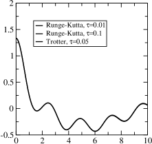
Figure 10: The value of $\langle S|^{-}(16,t)S^{+}(16,0)\rangle$ computed for a 31 site $S=1$ Heisenberg chain, computed three different times. Here the curves labeled Runge-Kutta are the TST method, implemented using Runge Kutta. The time step is $\tau$. The difference in results are not visible on this scale.

Both the Trotter method and the TST method give very accurate results. In Fig. 10 and Fig. 11, we show a comparison of the methods. On a large scale, we cannot see any difference between the methods for times out to $t\sim 10$. If we zoom in on a particular region, we see the effects of the finite Trotter decomposition error, here falling as $\tau^{2}$. We kept $m=300$ states for the TST method, and $m=200$ states for the Trotter methods. Typically, one finds that more states must be targetted for the TST method, because the targetting is over a finite interval of time rather than one instant. The Trotter decomposition error can be eliminated almost completely by using a higher order decomposition. In this case, the smaller value of $m$ still works as well as in the lower order methods. This combination gives the best combination of speed and accuracy.

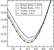
Figure 11: Same as for Fig. 10, but showing only a small region so the differences become apparent.

10 Spectral functions

Using either the Trotter or TST methods, it is straightforward to obtain spectral functions. Typically, we are interested in the Fourier transform of a time dependent correlation function

$$C(t)=\langle\phi|B(t)A(0)|\phi\rangle$$ (58)

where $|\phi\rangle$ is the ground state.

It is convenient to write this (cf. Eq. (20)) as

$$C(t)=\langle\phi|B\exp[-it(H-E_{G})]A|\phi\rangle$$ (59)

where $E_{G}$ is the ground state energy. For evaluating this expression, we proceed as follows: we first obtain the ground state using the standard DMRG algorithm. We then apply the operator $A$ to obtain $|\psi(t=0)\rangle$, and evolve $|\psi(t)\rangle$ in time, using the Hamiltonian with the ground state energy subtracted off. During this time evolution, we target both $|\psi(t)\rangle$ and $|\phi\rangle$. We then obtain $C(t)$, at each time step, as

$$C(t)=\langle\phi|B|\psi(t)\rangle.$$ (60)

By targetting both $|\psi(t)\rangle$ and $|\phi\rangle$, we ensure that this matrix element can be obtained with an accuracy controlled by the truncation error.

In forming $|\psi(t=0)\rangle$, we use a complete half-sweep to apply $A$ to $|\phi\rangle$. In particular, if $A$ is a sum of terms $A_{j}$ over a number of sites, then we apply an $A_{j}$ only when $j$ is one of the two central, untruncated sites. Thus the basis is automatically suitable for $A_{j}|\phi\rangle$. During this buildup of $A$ at step $j$ we target both $|\phi\rangle$ and $\sum_{j^{\prime}=1}^{j}A_{j^{\prime}}|\phi\rangle$. At the end of the sweep, we turn on the time evolution.

For translationally invariant systems it is particularly convenient to let $A$ and $B$ be on-site operators, for example $A=S^{+}(j)$, where $j$ is in the center of the chain. Since the time evolution does not evolve $B$, a whole set of $B$’s can be utilized, one for each site of the system, for example $B=S^{-}(\ell)$. One measurement of $G(\ell-j,t)$ can be made on each step of each sweep, where $\ell$ is one of the two center sites with untruncated bases, so that no extra operator matrices need be kept to reproduce $B$. In this way, one simulation yields $G(\ell-j,t)$ for a wide range of values of $\ell-j$ and $t$. By Fourier transforming in both space and time, one obtains the full spectral function for all frequency and momenta, in one simulation. This is in stark contrast to the most accurate frequency methods, in which one $k$ and a small range of $\omega$ are obtained in one run.

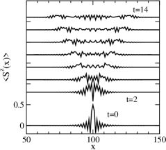
Figure 12: Time evolution of the local magnetization $\langle S^{z}(x)\rangle$ of a 200 site spin-1 Heisenberg chain after $S^{+}(100)$ is applied. From Whit04 .

As an example we return to the isotropic spin-1 Heisenberg chain, with the exchange coupling $J$ set to unity, and $A=S^{+}(j)$, as above. Note that the application of $S^{+}(j)$ constructs a localized wavepacket consisting of all wavevectors. This packet spreads out as time progresses, with different components moving at different speeds. The speed of a component is its group velocity, determined as the slope of the dispersion curve at $k$. In Fig.12 we show the local magnetization $\langle\psi(t)|S^{z}|\psi(t)\rangle$ for a chain of length $L=200$, with timestep $\tau=0.1$. At $t=0$, the wavepacket has a finite extent, with size given by the spin-spin correlation length $\xi$. At later times, the different speeds of the different components give the irregular oscillations in the center of the packet. We kept $m=150$ states per block, giving a truncation error of about $6\times 10^{-6}$. When the wavefront reaches the edge of the system, we stop the simulation. Our results up to that point in time have very minimal finite size effects, dying off exponentially from the edges. The correlation function is exponentially small for $|\ell-j|$ greater than $vt$, with $v$ the maximum group velocity. Because of this, we can specify the momentum precisely and arbitrarily, i.e. as if the system were infinite. The broadening from having a finite system appears only in frequency, not momentum.

The spectral function is defined as $-1/\pi{\rm Im}G(k,\omega)$, where

$$G(x,t)\equiv-iC(x,t)\equiv-i\langle\phi|T[S^{-}_{x}(t)S^{+}_{0}(0)]|\phi\rangle$$ (61)

Since $G(x,t)$ is even in $x$ and $t$, the Fourier transform is

$$G(k,\omega)=2\int_{0}^{\infty}dt\cos\omega t\sum_{x}\cos kxG(x,t)$$ (62)

In this expression, it is the real part of $C(x,t)$ that determines the spectral function; the imaginary part is thrown away. For an excited state with energy $\Delta$ above the ground state, this spectral function gives peaks at $\pm\Delta$. Alternatively, we can define the spectral function to have only the $+\Delta$ peaks. This spectral function comes from a Fourier transform utilizing both the real and imaginary parts of $C(x,t)$, and both positive and negative times:

$$A(k,\omega)=\frac{1}{2\pi}\int_{-\infty}^{\infty}dte^{i\omega t}\sum_{x}\cos kx\langle\phi|S^{-}_{x}(t)S^{+}_{0}|\phi\rangle.$$ (63)

In this case, we utilize $C(x,t)=C(x,-t)^{*}$ to obtain the negative time data. We prefer this latter spectral function, since it utilizes the imaginary data, but the differences are not large and we have not studied them carefully.

We approximate the time integral utilizing a windowing function $W(t)$ which goes to zero as $t\to T$,

$$\int_{-\infty}^{\infty}\approx\int_{-T}^{T}W(t).$$ (64)

A set of windowing functions with a number of nice properties is

$$W_{n}(t)=\cos(\frac{\pi t}{2T})^{n}.$$ (65)

These functions approach Gaussians as $n\to\infty$, but the function and $n-1$ derivatives vanish at $t=\pm T$. If one sets $W_{n}(t)$ to zero for $|t|>T$, and Fourier transforms, one obtains a nearly Gaussian lineshape with oscillating tails falling off as $\omega^{-(n+1)}$. We have used $n=4$, for which the lineshape in $\omega$ has negative regions in the tails of very small amplitude, less than half a percent of the peak height. Another good choice is $n=3$, giving a somewhat narrower peak at the expense of more negativity. Note that if the true spectral function has an isolated delta function peak, the windowed spectrum will have a broadened peak centered precisely at the same frequency. Thus it is possible to locate the single magnon line with an accuracy much better than $1/T$. If a continuum is also present nearby, the peak is less well determined. In the case of the $S=1$ chain, for $k$ near $\pi$ the peak is isolated, but at some point near $k=0.25\pi$ the peak enters the two magnon continuum and develops a finite width.

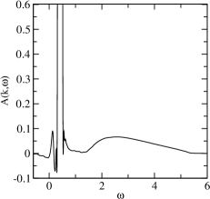
Figure 13: The single magnon spectrum of the spin-1 Heisenberg antiferromagnetic chain, for a system of $L=600$ sites, using the Trotter method with a time step of $\tau=0.1$, running for $T=100$, and keeping up to $m=600$ states, at momentum $k=\pi$. The main peak has a height of 83 at $\omega=0.415$, close to the true Haldane gap of $\Delta=0.41050(2)$.whitehuse The sharp oscillations around it are the result of numerical errors and windowing. The three-magnon continuum is visible, beginning at $3\Delta$.whitehuse

Figure 14: Same as for Fig. 13, but at $k=\pi/10$

In Fig.13 we show the resulting spectrum for $k=\pi$. The results for the three magnon continuum are impressive, as the single magnon line is much larger in amplitude. In Fig.14 we show results for $k=\pi/10$. For this momentum, the single magnon line lies within the two magnon continuum, altering its shape dramatically. This shape has been calculated approximately using the nonlinear sigma modelweston ; the results shown are in good qualitatively agreement with these analytic results.

11 Conclusion

While the invention of efficient time-dependent DMRG methods is at the time of writing only one and a half years old, the results achieved so far have already been impressive, indicating that the problem of highly precise time-evolutions for one-dimensional strongly correlated quantum is for the first time under very good control. The available variants cover a wide range of physical problems, with Trotter-based methods most efficient for short-ranged Hamiltonians, and with time-step targetting methods superior for longer-ranged interactions. They also provide powerful alternatives for the calculation of spectral functions in the momentum-frequency range. A nice feature is provided by their easy implementation in the framework of existing static finite-system DMRG codes. As control of quantum systems is improving experimentally, we expect the range of physical applications to grow strongly in the very near future.

References

- (1) M. Greiner, O. Mandel, T. Esslinger, T. W. Hänsch and I. Bloch, Nature (London) 415, 39 (2002)
- (2) M. Köhl, H. Moritz, T. Stöferle, K. Günter and T. Esslinger, Phys. Rev. Lett. 94, 080403 (2005)
- (3) S.R. White, Phys. Rev. Lett. 69, 2863 (1992)
- (4) S.R. White, Phys. Rev. B 48, 10345 (1993)
- (5) U. Schollwöck, Rev. Mod. Phys. 77, 259 (2005)
- (6) G. Vidal, Phys. Rev. Lett. 93, 040502 (2004)
- (7) A. J. Daley, C. Kollath, U. Schollwöck and G. Vidal, J. Stat. Mech.: Theor. Exp. (2004) P04005
- (8) S. R. White and A. Feiguin, Phys. Rev. Lett. 93, 076401 (2004)
- (9) A. Feiguin and S. R. White, Phys. Rev. B 72, 020404 (2005).
- (10) K. G. Wilson, Rev. Mod. Phys. 47, 773 (1975)
- (11) S. Östlund and S. Rommer, Phys. Rev. Lett. 75, 3537 (1995)
- (12) F. Verstraete, D. Porras and J. I. Cirac, Phys. Rev. Lett. 93, 227205 (2004)
- (13) K. Hallberg, Phys. Rev. B 52, 9827 (1995)
- (14) E. R. Gagliano and C. A. Balseiro, Phys. Rev. Lett. 59, 2999 (1987)
- (15) S. Ramasesha, S. K. Pati, H. R. Krishnamurthy, Z. Shuai, and J. L. Brédas, Synth. Met. 85, 1019 (1997)
- (16) T. Kühner and S.R. White, Phys. Rev. B 60, 335 (1999)
- (17) E. Jeckelmann, Phys. Rev. B 66, 045114 (2002)
- (18) Z. G. Soos and S. Ramasesha, J. Chem. Phys. 90, 1067 (1989)
- (19) M. Cazalilla and B. Marston, Phys. Rev. Lett. 88, 256403 (2002)
- (20) H. G. Luo, T. Xiang and X. Q. Wang, Phys. Rev. Lett. 91, 049701 (2003)
- (21) P. Schmitteckert, Phys. Rev. B 70, 121302 (2004)
- (22) G. Vidal, Phys. Rev. Lett. 91, 147902 (2003)
- (23) M. Fannes, B. Nachtergaele and R. F. Werner, Comm. Math. Phys. 144, 3 (1992)
- (24) A. Klümper and A. Schadschneider and J. Zittartz, Europhys. Lett. 24, 293 (1993)
- (25) M. Suzuki, Prog. Theor. Phys. 56, 1454 (1976)
- (26) S. R. White, Phys. Rev. Lett. 77, 3633 (1996)
- (27) D. Gobert, C. Kollath, U. Schollwöck and G. Schütz, Phys. Rev. E 71, 036102 (2005)
- (28) T. Antal, Z. Racz, A. Rakos, G. Schütz, Phys. Rev. E 59, 4912 (1999)
- (29) F. Verstraete, J. J. Garcia-Rípoll and J. I. Cirac, Phys. Rev. Lett. 93, 207204 (2004)
- (30) C. Kollath, U. Schollwöck, J. von Delft and W. Zwerger, Phys. Rev. A 71, 053606 (2005)
- (31) C. Kollath, U. Schollwöck and W. Zwerger, Phys. Rev. Lett. 95, 176401 (2005)
- (32) S. Trebst, U. Schollwöck, M. Troyer and P. Zoller, cond-mat/0506809
- (33) M. Zwolak and G. Vidal, Phys. Rev. Lett. 93, 207205 (2004)
- (34) A. Bühler, N. Elstner and G. S. Uhrig, Eur. Phys. J. B 16, 475 (2000)
- (35) S.R. White and D.A. Huse, Phys. Rev. B 48, 3844 (1993).
- (36) I. Affleck and R.A. Weston, Phys. Rev. B 45, 4667 (1992).