Universal phase diagram of a strongly interacting Fermi gas with unbalanced spin populations.

Abstract

We present a theoretical interpretation of a recent experiment presented in ref. Zwierlein06 on the density profile of Fermi gases with unbalanced spin populations. We show that in the regime of strong interaction, the boundaries of the three phases observed in Zwierlein06 can be characterized by two dimensionless numbers $\eta_{\alpha}$ and $\eta_{\beta}$. Using a combination of a variational treatment and a study of the experimental results, we infer rather precise bounds for these two parameters.

I Introduction

In fermionic systems, superfluidity arises from the pairing of two particles with opposite spin states, a scenario first pointed out by Bardeen Cooper and Schrieffer (BCS) to explain the onset of superconductivity in metals. For this mechanism to be efficient, the Fermi surfaces associated with each spin component need be matched, and soon after the seminal BCS work the question of the effect of a population imbalance between the two states was raised. At the time, it was understood that pairing and superfluidity could sustain a certain amount of mismatch, above which the system would undergo a quantum phase transition towards a normal state Clogston62 . The original work of Fulde, Ferrel, Larkin and Ovchinnikov, who proposed the existence of Cooper pairing at finite momentum, was later generalized to trapped systems Combescot05 . Alternative scenarios were also proposed, including deformed Fermi surfaces Sedrakian05 , interior gap superfluidity Liu03 , phase separation between a normal and a superfluid state through a first order phase transition Bedaque03 , BCS quasi-particle interactions Ho06 or onset of p-wave pairing Bulgac06 . When the strength of the interactions is varied, a complicated phase diagram mixing several of these scenarios is expected Pao05 .

However, due to the absence of experimental evidence, these scenarios could never be tested experimentally until the subject was revived by the possibility of reaching superfluidity in ultra-cold fermionic gaseous systems Jochim03 ; Bourdel04 . Contrarily to usual condensed matter systems, spin relaxation is very weak in cold atoms, and this allows one to keep spin polarized samples for long times. This unique possibility led to the first experimental studies of imbalanced Fermi gases at MIT and Rice University Zwierlein05 ; Partridge05 ; Zwierlein06 . These results triggered a host of theoretical work aiming at explaining the various results observed by the two groups Pieri05 ; Chevy06 .

One remarquable feature of ref. Zwierlein06 is the observation of three different phases in the cloud. At the center, the authors observe a superfluid core, where the densities of the two spin states are equal, then an intermediate normal shell where the two states coexist and finally an outer rim of the majority component. In the present paper, we show that, though performed in a trap, the observations of MIT can offer valuable information on the phase diagram of a strongly interacting Fermi gas with unbalanced populations. In a first part we will present a brief overview of the simplest free space scenario for transition from a paired superfluid to a pure normal state, through a mixed phase. Focusing on the disappearance of the minority component, we will present a variational study of the problem of a single minority particle embedded in the Fermi sea of majority atoms. Finally, we will show that the comparison with experiments allows for a rather precise determination of the transition thresholds. One of the key point is that, contrarily to previous works, we rely on universal thermodynamics Ho03 as well as “exact” experimental or Monte Carlo results, without the need of the mean field BCS ansatz often used in other publications, an approach similar to that of Bulgac .

II Homogeneous system

Before addressing the case of trapped fermions, let us first discuss their free space phase diagram. We consider zero temperature fermions of mass $m$ with two internal states labelled 1 and 2. Within a quantization volume $V$ and in the limit of short range interactions, we can write the hamiltonian of the system as

$$\widehat{H}=\sum_{\bm{k},\sigma}\epsilon_{\bm{k}}\widehat{a}_{\bm{k},\sigma}^{\dagger}\widehat{a}_{\bm{k},\sigma}+\frac{g_{\rm b}}{V}\sum_{\bm{k},\bm{k}^{\prime},\bm{q}}\widehat{a}^{\dagger}_{\bm{k}+\bm{q},1}\widehat{a}_{\bm{k}^{\prime}-\bm{q},2}^{\dagger}\widehat{a}_{\bm{k}^{\prime},2}\widehat{a}_{\bm{k},1}.$$ (1)

Here, $\epsilon_{\bm{k}}=\hbar^{2}k^{2}/2m$, $\widehat{a}_{\bm{k},\sigma}$ is the annihilation operator of a species $\sigma$ particle with momentum $\bm{k}$, and $g_{\rm b}$ is the bare coupling constant characterizing inter-particle interactions. It is related to the s-wave scattering length of the system $a$ by the Lippmann-Schwinger equation

$$\frac{1}{g_{\rm b}}=\frac{m}{4\pi\hbar^{2}a}-\frac{1}{V}\sum_{\bm{k}}\frac{1}{2\epsilon_{\bm{k}}}.$$ (2)

We note that only interactions between particles of opposite spins are taken into account, due to the Pauli principle which forbids s-wave scattering of atoms with identical spin. In this paper, we assume we are working at the unitary limit where $|a|=\infty$ and, using the grand canonical ensemble, we wish to find the ground state of the grand-potential $\widehat{\Xi}=\widehat{H}-\mu_{1}\widehat{N}_{1}-\mu_{2}\widehat{N}_{2}$. Here $\widehat{N}_{i}$ is the particle number operator for species $i$ and $\mu_{i}$ is the associated chemical potential (we take species 1 as majority hence $\mu_{1}>\mu_{2}$). The grand potential can be expressed as the function of the volume $V$ and pressure $P$ of the ensemble according to $\langle\widehat{\Xi}\rangle=-PV$. In other words, searching the ground state of the system is equivalent to searching the phase with the highest pressure $P$.

To start our analysis, we note first that two exact eigenstates of $\widehat{\Xi}$ can be found quite easily. First, when the gas is fully polarized, we recover the case of an ideal Fermi gas for which we know that

$$P_{\rm N}=\frac{1}{15\pi^{2}}\left(\frac{2m}{\hbar^{2}}\right)^{3/2}\mu_{1}^{5/2}.$$

Second, let us now consider the exact ground state $|{\rm SF}\rangle_{\mu}$ of the balanced grand potential $\widehat{\Xi}^{\prime}=\widehat{H}-\mu(\widehat{N}_{1}+\widehat{N}_{2})$, describing a superfluid with chemical potential $\mu$. This potential commutes with the number operators, hence the ground state can be searched as an eigenstate for both $\widehat{N}_{1}$ and $\widehat{N}_{2}$, with $\widehat{N}_{1}|{\rm SF}\rangle_{\mu}=\widehat{N}_{2}|{\rm SF}\rangle_{\mu}$. We check readily that $|{\rm SF}\rangle_{\bar{\mu}}$, with $\bar{\mu}=(\mu_{1}+\mu_{2})/2$, is still an eigenstate of the unbalanced $\widehat{\Xi}$, by noting that $\widehat{\Xi}=\widehat{\Xi}^{\prime}+(\mu_{1}-\mu_{2})(\widehat{N}_{1}-\widehat{N}_{2})/2$. At unitarity the pressure of a balanced Fermi gas reads $P_{\rm S}=2\left(2m/\xi\hbar^{2}\right)^{3/2}\mu^{5/2}/15\pi^{2}$, where $\xi\sim 0.42$ is a universal parameter whose determination has attracted interest of both theoreticians Carlson03 ; Perali04 ; Carlson05 ; Astrakharchik04 and experimentalists Bourdel04 ; OHara02 . In the case of mismatched chemical potentials, the pressure of this fully paired superfluid state is therefore

$$P_{S}=\frac{1}{15\pi^{2}}\left(\frac{m}{\xi\hbar^{2}}\right)^{3/2}(\mu_{1}+\mu_{2})^{5/2}.$$

The evolution of $P_{N}$ and $P_{S}$ is presented in Fig. 1 as a function of $\eta=\mu_{2}/\mu_{1}$. We see that they cross for $\eta_{\rm c}=(2\xi)^{3/5}-1\sim-0.10$, marking the instability of the superfluid against large population imbalances Chevy06 . However, since we only compare the energy of the fully paired state to the one of the fully polarized ideal gas, the real breakdown of superfluidity could very well happen for some $\eta$ larger than $\eta_{c}$. We know this is actually the case, since in ref. Zwierlein06 , the authors observed an intermediate normal phase, containing atoms of both species. From universality at unitarity, the phase transition from the fully paired to the intermediate phase, and then from the intermediate to the fully polarized normal phase are given by conditions $\mu_{2}/\mu_{1}=\eta_{\alpha}$, and $\mu_{2}/\mu_{1}=\eta_{\beta}$, where $\eta_{\alpha}$ and $\eta_{\beta}$ are two universal parameters we would like to determine as precisely as possible.

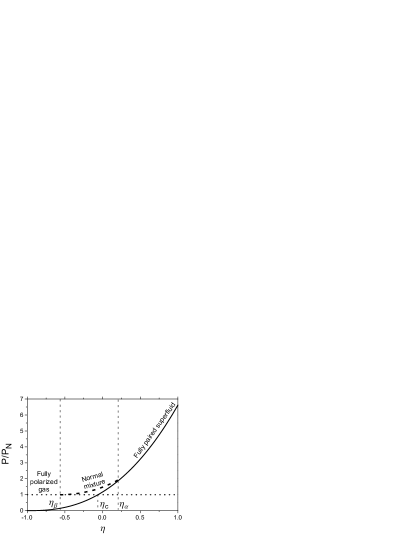
Figure 1: Comparison of the pressure of the various phases, normalized by the pressure $P_{N}$ of the fully polarized ideal Fermi gas, as a function of the chemical potential mismatch $\eta=\mu_{2}/\mu_{1}$. Dotted line: fully polarized phase. Full line: fully paired superfluid phase. The fully paired and fully polarized states meet for $\eta_{c}\sim-0.099$. Dashed line: sketch of the intermediate normal phase. $\eta_{\alpha}$ and $\eta_{\beta}$ designate the universal chemical potential thresholds for this phase.

Noting that the transition from the fully paired state to the intermediate one must happen before the transition to the fully polarized phase, we see graphically that we have necessarily $\eta_{\alpha}>\eta_{c}$, and, similarly, $\eta_{\beta}<\eta_{c}$. The upper bound on $\eta_{\beta}$ can be further improved by noting that at the threshold between the normal mixture and the fully polarized ideal gas, there are only a few atoms of the minority species. In principle, the value of $\eta_{\beta}$ should then be found by studying the N+1 body problem of a Fermi sea of N particles 1, in presence of a single minority atom. To address this problem, we use here a variational method inspired from first order perturbation theory, where we expect the ground state of the system to take the form

$$|\psi\rangle=\phi_{0}|{\rm FS}\rangle+\sum_{\bm{k},\bm{q}}\phi_{\bm{k},\bm{q}}|\bm{k},\bm{q}\rangle,$$

where $|{\rm SF}\rangle$ is a non interacting majority Fermi sea plus a minority atom with 0 momentum, and $|\bm{k},\bm{q}\rangle$ is the perturbed Fermi sea with a majority atom with momentum $\bm{q}$ (with $q$ lower than $k_{F}$) excited to momentum $\bm{k}$ (with $k>k_{F}$). To satisfy momentum conservation, the minority atom acquires a momentum $\bm{q}-\bm{k}$. The energy of this state with respect to the non interacting ground state is $\langle\widehat{\Delta}H\rangle=\langle\widehat{H}_{0}\rangle+\langle\widehat{V}\rangle$, with

$$\langle\widehat{H}_{0}\rangle=\sum_{\bm{k},\bm{q}}|\phi_{\bm{k},\bm{q}}|^{2}(\epsilon_{\bm{k}}+\epsilon_{\bm{q}-\bm{k}}-\epsilon_{\bm{q}}),$$

and

$$\langle\widehat{V}\rangle = \frac{g_{b}}{V}\left(\sum_{\bm{q}}|\phi_{0}|^{2}+\sum_{\bm{k},\bm{k}^{\prime},\bm{q}}\phi_{\bm{k}^{\prime},\bm{q}}\phi^{*}_{\bm{k},\bm{q}}+\sum_{\bm{k},\bm{q},\bm{q}^{\prime}}\phi_{\bm{k},\bm{q}}\phi^{*}_{\bm{k},\bm{q}^{\prime}}\right.$$

$$\left.+\sum_{\bm{q},\bm{k}}(\phi^{*}_{0}\phi_{\bm{k},\bm{q}}+\phi_{0}\phi^{*}_{\bm{k},\bm{q}})\right),$$

where the sums on $q$ and $k$ are implicitly limited to $q<k_{F}$ and $k>k_{F}$. As we will check later (see below, eqn. (3)), $\phi_{\bm{k},\bm{q}}\sim 1/k^{2}$ for large momenta, in order to satisfy the short range behavior $1/r$ of the pair wave function in real space. This means that most of the sums on $\bm{k}$ diverge for $k\rightarrow\infty$. This singular behavior is regularized by the renormalization of the coupling constant using the Lippman-Schwinger formula, thus yielding a vanishing $g_{B}$. As a consequence, since the third sum in $\langle\widehat{V}\rangle$ is convergent, it gives a zero contribution to the final energy when multiplied by $g_{B}$, and can therefore be omitted in the rest of the calculation.

The minimization of $\langle\widehat{H}\rangle$ with respect to $\phi_{0}$ and $\phi_{\bm{k},\bm{q}}$ is straightforward and yields the following set of equations

$$(\epsilon_{\bm{k}}+\epsilon_{\bm{q}-\bm{k}}-\epsilon_{\bm{q}})\phi_{\bm{k},\bm{q}}+\frac{g_{b}}{V}\sum_{\bm{k}^{\prime}}\phi_{\bm{k}^{\prime},\bm{q}}+\frac{g_{b}}{V}\phi_{0} = E\phi_{\bm{k},\bm{q}},$$

$$\frac{g_{b}}{V}\sum_{\bm{q}}\phi_{0}+\frac{g_{b}}{V}\sum_{\bm{q},\bm{k}}\phi_{\bm{k},\bm{q}} = E\phi_{0}$$

where $E$ is the Lagrange multiplier associated to the normalization of $|\psi\rangle$, and can also be identified with the trial energy. These equations can be solved self consistently by introducing an auxiliary function $\chi(\bm{q})=\phi_{0}+\sum_{\bm{k}}\phi_{\bm{k},\bm{q}}$ and we obtain

$$\phi_{\bm{k},\bm{q}}=\frac{g_{B}\chi(\bm{q})/V}{E-(\epsilon_{\bm{k}}+\epsilon_{\bm{q}-\bm{k}}-\epsilon_{\bm{q}})},$$ (3)

After a straightforward calculation, this yields

$$E=\sum_{q<k_{F}}\frac{1}{\sum_{k>k_{F}}\left(\frac{1}{\epsilon_{\bm{k}}+\epsilon_{\bm{q}-\bm{k}}-\epsilon_{\bm{q}}-E}-\frac{1}{2\epsilon_{\bm{k}}}\right)-\sum_{k<k_{F}}\frac{1}{2\epsilon_{\bm{k}}}}.$$

where we got rid of the bare coupling constant $g_{B}$ by using the Lippman-Schwinger equation (2). This equation can be solved numerically and yields $E=-0.3\hbar^{2}k_{F}^{2}/m$, i.e. $\eta_{\beta}<-0.6$ Lobo06 . Note that the same analytical result was obtained independently in Combescot06 .

III Trapped system and comparison with experiments

In the rest of the paper, we would like to show how experimental data from ref. Zwierlein06 permits to improve the determination of the parameters $\eta_{\alpha,\beta}$ . In this pursuit, we use the Local Density Approximation (LDA) to calculate the density profile of the cloud in a harmonic trap, which for simplicity we assume is isotropic. In this case, the chemical potentials $\mu_{1,2}$ of each species depends on position according to the law $\mu_{1,2}(\bm{r})=\mu_{1,2}^{0}-m\omega^{2}r^{2}/2$, where $\omega$ is the trap frequency.

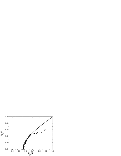
Figure 2: Comparison between experimental data of ref. Zwierlein06 (squares) and eq. (4) (full line). $R_{\alpha}$, $R_{\beta}$ and $R_{1}$ are respectively the radii of the superfluid, minority and majority components. The condensate vanishes for $R_{\alpha}=0$ at $q=R_{\beta}^{2}/R_{1}^{2}\sim 0.32$.

Using this assumption, the transition between the various phases will happen at radii $R_{\alpha}$ and $R_{\beta}$ given by $\mu_{2}(R_{\alpha,\beta})/\mu_{1}(R_{\alpha,\beta})=\eta_{\alpha,\beta}$. When these two equations are associated with the condition giving the radius $R_{1}$ of the majority component, $\mu_{1}(R_{1})=0$, we can eliminate both $\mu_{1}^{0}$ and $\mu_{2}^{0}$ from the equations, yielding the following close formula relating the radii $R_{\alpha}$, $R_{\beta}$ and $R_{1}$

$$\frac{R_{\alpha}}{R_{1}}=\sqrt{\frac{(R_{\beta}/R_{1})^{2}-q}{1-q}}.$$ (4)

Here, $q=(\eta_{\alpha}-\eta_{\beta})/(1-\eta_{\beta})$ corresponds to the value of the $R_{\beta}^{2}/R_{1}^{2}$ at which $R_{\alpha}$ vanishes, i.e. at which the superfluid fraction disappears. In Fig. 2, we compare the prediction of eq. 4 with the experimental finding of ref. Zwierlein06 , taking $q=0.32$ to match the superfluidity thresholds. We see that close to the threshold, the agreement between the two graphs is quite good. However, they depart from each other for $R_{\beta}/R_{1}\gtrsim 0.7$, corresponding to low population imbalance. One explanation for this discrepancy might involve finite temperature effects. Indeed, it was already noted in Fig. 4 of ref. Zwierlein05 that, although the superfluid fraction was very sensitive to temperature at small imbalances, the value of the critical population imbalance was more robust.

The superfluid phase disappears when $R_{\alpha}$ vanishes. From eq. 4, we see this happens for a ratio $R^{2}_{\beta}/R^{2}_{1}=q$. As seen in Fig. 2, $q$ can be extracted from the experimental data of ref. Zwierlein06 , which yield $q\sim 0.32$ and therefore constrain the possible values of $\eta_{\alpha}$ and $\eta_{\beta}$. Indeed, using this determination of $q$, as well as the rough upper and lower values for $\eta_{\alpha,\beta}$, one obtains

$$-0.10<\eta_{\alpha}<-0.088$$ (5)

$$-0.62<\eta_{\beta}<-0.60$$ (6)

These bounds can be compared to the values deduced by BCS theory, predicting $\eta_{\alpha}\sim 0.1$ and $\eta_{\beta}=0$. Our calculation excludes these values and explains why the width of the mixed normal state predicted by BCS theory is much narrower than observed in experiments.

IV Conclusion

In conclusion, we have presented an analysis of the experimental data of ref. Zwierlein06 providing stringent bounds on the values of the thresholds for quantum phase transitions in uniform unbalanced fermi gases. Since they were obtained using minimal assumptions (mainly zero temperature and LDA), these bounds are fairly robust. In particular, they do not depend precisely on the superfluid nature of the intermediate phase. Our results suggest interesting follow-ups. First, the full understanding of the system, and in particular of the density profile of the cloud, requires the knowledge of the state equation of the intermediate phase, whose exact nature then needs to be clarified. Second, the comparison with the data of ref. Partridge05 suggests an intriguing issue. Indeed, although the superfluidity threshold was not directly measured in this paper, the parameter $q$ can be inferred from the critical imbalance 0.7 measured by MIT. Rice’s experimental data yield at this value $q\sim 0.16$. Not only is this value very far from the one obtained here from the analysis of MIT’s experiments, but it also contradicts the theoretical bounds $\eta_{\alpha}>-0.10$ and $\eta_{\beta}<-0.60$ which imply $q>0.31$. As suggested in ref. Silva06b , this discrepancy may arise from surface tension effects provoked by the strong anisotropy of Rice’s trap. Another interpretation might be the onset of the intermediate phase due to finite temperature effects, as suggested by some mean-field scenarios. Finally, the $\eta_{\alpha,\beta}$ parameters can be evaluated experimentally using the value of $q$ associated with the measurement of the density discontinuity $\Delta n_{1,2}$ at $r=R_{\alpha}$, given by $\Delta n_{1}/\Delta n_{2}=-\eta_{\alpha}$ Footnote . The preliminary data presented in fig. 2.b of ref. Zwirlein06c suggest that the discontinuity $\Delta n_{1}$ is very weak, hence indicating a small value of $\eta_{\alpha}$, in agreement with the bounds obtained here.

- (1) B.S. Chandrasekhar, Appl. Phys. Lett. 1 ,7 (1962), A. M. Clogston, Phys. Rev. Lett. 9, 266 (1962); G. Sarma, Journal of Physics and Chemistry of Solids 24, 1029 (1963); P. Fulde, R. A. Ferrell, Phys. Rev. 135, A550 (1964); J. Larkin, Y. N. Ovchinnikov, Sov. Phys. JETP 20, 762 (1965).
- (2) R. Combescot, Europhys. Lett. 55 (2),150 (2001); C. Mora and R. Combescot, Phys. Rev. B. 71, 214504. (2005); P. Castorina, M. Grasso, M. Oertel, M. Urban, and D. Zappalà Phys. Rev. A 72, 025601 (2005); T. Mizushima, K. Machida, and M. Ichioka, Phys. Rev. Lett. 94, 060404 (2005); T. Mizushima, K. Machida, and M. Ichioka, Phys. Rev. Lett. 95, 117003 (2005); K. Machida, T. Mizushima, and M. Ichioka, Phys. Rev. Lett. 97, 120407 (2006) .
- (3) A. Sedrakian, J. Mur-Petit, A. Polls, and H. Müther, Phys. Rev. A 72, 013613 (2005).
- (4) W.V. Liu and F. Wilczek, Phys. Rev. Lett. 90, 047002 (2003).
- (5) P.F. Bedaque, H. Caldas, and G. Rupak, Phys. Rev. Lett. 91 247002 (2003); H. Caldas, Phys. Rev. A 69, 063602 (2004); T.D. Cohen, Phys. Rev. Lett. 95, 120403 (2005).
- (6) J. Carlson and S. Reddy, Phys. Rev. Lett. 95, 060401 (2005);
- (7) T.-L. Ho and H. Zai, cond-mat/0602568.
- (8) A. Bulgac, M. McNeil Forbes, and A. Schwenk, Phys. Rev. Lett. 97, 020402 (2006).
- (9) C.H. Pao, Shin-Tza Wu and S.-K. Yip, Phys. Rev. B 73, 132506 (2006); D.T Son and M.A. Stephanov, Phys. Rev. A 74, 013614 (2006); D.E. Sheehy and L. Radzihovsky, Phys. Rev. Lett. 96, 060401 (2006).
- (10) S. Jochim, M. Bartenstein, A. Altmeyer, G. Hendl, S. Riedl, C. Chin, J. H. Denschlag, and R. Grimm, Science 302, 2101 (2003); M. W. Zwierlein, C. A. Stan, C. H. Schunck, S. M. F. Raupach, S. Gupta, Z. Hadzibabic, and W. Ketterle, Phys. Rev. Lett. 91, 250401 (2003); M. Greiner, C. A. Regal, and D. S Jin, Nature 426, 537 (2003); J. Kinast, S. L. Hemmer, M. E. Gehm, A. Turlapov, and J. E. Thomas, Phys. Rev. Lett. 92, 150402 (2004); G. B. Partridge, K. E. Strecker, R. I. Kamar, M. W. Jack, and R. G. Hulet, Phys. Rev. Lett. 95, 020404 (2005).
- (11) T. Bourdel, L. Khaykovich, J. Cubizolles, J. Zhang, F. Chevy, M. Teichmann, L. Tarruell, S. J. J. M. F. Kokkelmans, and C. Salomon, Phys. Rev. Lett. 93, 050401 (2004).
- (12) M. W. Zwierlein, A. Schirotzek, C. H. Schunck, and W. Ketterle, Science 311, 492 (2006).
- (13) G. B. Partridge, W. Li, R. I. Kamar, Y. Liao, and R. G. Hulet, Science 311, 503 (2006).
- (14) M. W. Zwierlein, C. H. Schunck, A. Schirotzek, W. Ketterle, Nature 442, 54 (2006).
- (15) P. Pieri, G.C. Strinati, Phys. Rev. Lett. 96, 150404 (2006); W. Yi and L.-M. Duan, Phys. Rev. A 73, 031604(R) (2006); T. N. De Silva, and E. J. Mueller, Phys. Rev. A 73, 051602 (R) (2006); M. Haque, and H.T.C. Stoof, Phys. Rev. A 74, 011602 (2006); H. Hu and X.-J. Liu, Phys. Rev. A 73 051603(R) (2006).
- (16) F. Chevy, Phys. Rev. Lett. 96, 130401 (2006).
- (17) T.L. Ho Phys. Rev. Lett. 92, 090402 (2004).
- (18) A. Bulgac and M. McNeil Forbes, e-print cond-mat/0606043.
- (19) J. Carlson, S.-Y. Chang, V. R. Pandharipande, and K. E. Schmidt , Phys. Rev. Lett. 91, 050401 (2003).
- (20) G. E. Astrakharchik, J. Boronat, J. Casulleras, S. Giorgini, Phys. Rev. Lett. 93, 200404 (2004).
- (21) A. Perali, P. Pieri, G. C. Strinati, Phys. Rev. Lett. 93, 100404 (2004).
- (22) K. M. O’Hara, S. L. Hemmer, M. E. Gehm, S. R. Granade, and J. E. Thomas, Science 298, 2179 (2002); M. Bartenstein, A. Altmeyer, S. Riedl, S. Jochim, C. Chin, J. Hecker Denschlag, and R. Grimm, Phys. Rev. Lett. 92, 120401 (2004); J. Kinast, A. Turlapov, J. E. Thomas, Q. Chen, J. Stajic, and K. Levin, Science 307, 1296 (2005).
- (23) T.N. De Silva and E.J. Mueller, Phys. Rev. Lett. 97, 070402 (2006).
- (24) This result is obtained by assuming the universal form , with , and using the continuity of pressure and chemical potentials at the transition.
- (25) M.W. Zwierlein and W. Ketterle, e-print cond-mat/0603489.
- (26) We note that the upper bound found here is very close to the result of recent Monte Carlo simulations presented in C. Lobo C. Lobo, A. Recati, S. Giorgini, and S. Stringari, e-print cond-mat/0607730.
- (27) R. Combescot, private communication, to be published.