Finite temperature phase diagram of a polarised Fermi condensate

Abstract

The two-component Fermi gas is the simplest fermion system displaying superfluidity, and as such is relevant to topics ranging from superconductivity to QCD. Ultracold atomic gases provide an exceptionally clean realisation of this system, where interatomic interactions and atom spin populations are both independently tuneable. Here we show that the finite temperature phase diagram contains a region of phase separation between the superfluid and normal states that touches the boundary of second-order superfluid transitions at a tricritical point, reminiscent of the phase diagram of ³He-⁴He mixtures. A variation of interaction strength then results in a line of tricritical points that terminates at zero temperature on the molecular Bose-Einstein condensate (BEC) side. On this basis, we argue that tricritical points are fundamental to understanding experiments on polarised atomic Fermi gases.

Over the past decade, experimental progress in the field of cold atomic gases has resulted in unprecedented control over pairing phenomena in two-component Fermi gases. The ability to vary the effective interaction between atoms using magnetically tuned Feshbach resonances has already permitted the experimental investigation of the crossover from a BEC of diatomic molecules to the Bardeen-Cooper-Schrieffer (BCS) limit of weakly-bound Cooper pairs of fermionic atoms Regal et al. (2004); Zwierlein et al. (2004); Chin et al. (2004); Bourdel et al. (2004); Kinast et al. (2004); Zwierlein et al. (2005). A natural extension of these studies is an exploration of the Fermi gas with imbalanced spin populations, especially since this system has a far richer phase diagram than the equal spin case. As well as exhibiting a quantum phase transition between the superfluid and normal states, the polarized Fermi gas has been predicted to possess exotic superfluid phases such as the inhomogeneous Fulde-Ferrell-Larkin-Ovchinnikov (FFLO) state Fulde and Ferrell (1964); Larkin and Ovchinnikov (1965), where the pairing of fermions occurs at finite centre-of-mass momentum, and the deformed Fermi surface state Sedrakian et al. (2005). The exact nature of the superfluid states for the polarised Fermi gas is still the subject of considerable debate. However, atomic gases provide an ideal testing ground for this system, since the particle numbers can be varied independently from all other experimental parameters, and pioneering experiments have recently been performed Zwierlein et al. (2006a); Partridge et al. (2006); Zwierlein et al. (2006b); Shin et al. (2006). Contrast atomic gases with the case of superconductors, where the magnetic field used to generate a spin imbalance (via the Zeeman effect) also couples to orbital degrees of freedom.

In this work, we elucidate the finite temperature phase diagram of a polarised Fermi gas. While much insight has been gained from previous theoretical studies Bedaque et al. (2003); Carlson and Reddy (2005); Pao et al. (2006); Son and Stephanov (2006); Mizushima et al. (2005); Sheehy and Radzihovsky (2006); Mannarelli et al. ; Pieri and Strinati (2006); Liu and Hu (2006); Hu and Liu (2006); Chien et al. (2006); Gu et al. ; Martikainen (2006); Iskin and Sá de Melo ; De Silva and Mueller (2006a); Haque and Stoof (2006); Yi and Duan (2006a); Kinnunen et al. (2006), so far a key ingredient of the phase diagram has been overlooked: the tricritical point, at which the phase transition between superfluid and normal states switches from first to second order. By determining the behaviour of the tricritical point as a function of interaction strength, we can completely characterise the topology of the phase diagram without recourse to an extensive numerical treatment. Specifically, we shall focus on the uniform, infinite system, and concern ourselves almost exclusively with the phase boundary between the normal and homogeneous superfluid states. We will, however, discuss the ramifications of the inferred phase diagram for the trapped system.

I Formalism

Experiments to date exploit wide Feshbach resonances and are thus well described by the simplest single-channel Hamiltonian, where the two fermion species interact via an attractive contact potential

$$\hat{H}-\mu_{\uparrow}\hat{n}_{\uparrow}-\mu_{\downarrow}\hat{n}_{\downarrow}=\sum_{{\mathbf{k}}}\sum_{\sigma=\uparrow,\downarrow}\left(\epsilon_{{\mathbf{k}}}-\mu_{\sigma}\right)c_{{\mathbf{k}}\sigma}^{\dagger}c_{{\mathbf{k}}\sigma}\\ +\frac{g}{V}\sum_{{\mathbf{k}},{\mathbf{k}}^{\prime},{\mathbf{q}}}c_{{\mathbf{k}}+{\mathbf{q}}/2\uparrow}^{\dagger}c_{-{\mathbf{k}}+{\mathbf{q}}/2\downarrow}^{\dagger}c_{-{\mathbf{k}}^{\prime}+{\mathbf{q}}/2\downarrow}c_{{\mathbf{k}}^{\prime}+{\mathbf{q}}/2\uparrow}\;.$$ (1)

Here, $\epsilon_{{\mathbf{k}}}={{\mathbf{k}}}^{2}/2m_{f}$ (we set $\hbar=1$ and $k_{B}=1$), $V$ is the volume, and we define the chemical potential $\mu$ and ‘Zeeman’ field $h$ such that $\mu_{\uparrow}=\mu+h$ and $\mu_{\downarrow}=\mu-h$. At present, only pairing between different hyperfine species of the same atom has been explored experimentally, so we restrict ourselves to a single mass $m_{f}$. The interaction strength $g$ is expressed in terms of the s-wave scattering length $a$ using the prescription:

$$\frac{m_{f}}{4\pi a}=\frac{1}{g}+\frac{1}{V}\sum_{{\mathbf{k}}}\frac{1}{2\epsilon_{{\mathbf{k}}}}\;.$$

We also derive the Fermi momentum using the average density $n/2\equiv(n_{\uparrow}+n_{\downarrow})/2$, so that $k_{F}=(3\pi^{2}n)^{1/3}$. Throughout our calculations, we will keep $n$ fixed.

The full phase diagram is parameterised by just a few observables: the temperature $T\equiv 1/\beta$, the interaction strength $1/k_{F}a$, and the density difference or ‘magnetisation’ $m\equiv n_{\uparrow}-n_{\downarrow}$. To determine the position of the phase boundaries, we must minimise the mean-field free energy density

$$\Omega^{0}=-\frac{\Delta^{2}}{g}+\frac{1}{V}\sum_{{\mathbf{k}}}(\xi_{{\mathbf{k}}}-E_{{\mathbf{k}}})\\ -\frac{1}{\beta V}\sum_{{\mathbf{k}}}\left[\ln\left(1+e^{-\beta(E_{{\mathbf{k}}}-h)}\right)+\ln\left(1+e^{-\beta(E_{{\mathbf{k}}}+h)}\right)\right],$$ (2)

with respect to the BCS order parameter $\Delta$, where $\xi_{{\mathbf{k}}}=\epsilon_{{\mathbf{k}}}-\mu$ and $E_{{\mathbf{k}}}=\sqrt{\xi_{{\mathbf{k}}}^{2}+\Delta^{2}}$. Such a mean-field analysis provides a reasonable description of the zero temperature phase diagram, but at finite temperature, it neglects the contribution of non-condensed pairs to both the density $n=-\partial\Omega/\partial\mu$ and magnetisation $m=-\partial\Omega/\partial h$. This contribution is necessary to approach the transition temperature of an ideal Bose gas in the molecular limit, and can be included in the non-condensed phase ($\Delta=0$) through the Nozières-Schmitt-Rink (NSR) fluctuation correction to the energy Noziéres and Schmitt-Rink (1985)

$$\left.\Omega^{1}\right|_{\Delta=0}=\frac{1}{\beta V}\sum_{{\mathbf{q}},i\omega}\ln\Gamma^{-1}({\mathbf{q}},i\omega)\;,$$ (3)

with

$$\Gamma^{-1}({\mathbf{q}},i\omega)=-\frac{1}{g}\\ -\frac{1}{2V}\sum_{{\mathbf{p}}}\frac{\tanh{[\frac{\beta}{2}(\xi_{{\mathbf{p}}}+h)]+\tanh[\frac{\beta}{2}(\xi_{{\mathbf{p}}+{\mathbf{q}}}-h)]}}{i\omega+\xi_{{\mathbf{p}}}+\xi_{{\mathbf{p}}+{\mathbf{q}}}}\;.$$ (4)

This gives an estimate of the effect of pair fluctuations on the second order phase boundary (but not the first order boundary, where $\Delta\neq 0$).

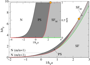
Figure 1: The zero temperature phase diagram within mean-field theory for both Zeeman field $h/\varepsilon_{F}$ and magnetisation $m/n$ (inset) versus interaction $1/k_{F}a$. There are four different phases: the normal (N) state, the phase-separated (PS) state, the ordinary superfluid (SF) and the magnetised superfluid (SF${}_{\textrm{M}}$). Above the line $h/\varepsilon_{F}=2^{-1/3}$, the normal state is completely polarised ($m/n=1$). The red and black lines enclosing the PS state are both first-order phase boundaries, while the SF${}_{\textrm{M}}$-N transition is second-order, and the SF-SF${}_{\textrm{M}}$ transition (green line) is at least third-order. The tricritical point is represented by orange circles at $1/k_{F}a=2.368$ with $h/\varepsilon_{F}=6.876$ or $m/n=1$.

II Phase diagram for the uniform case

Considerable insight can be gained by first examining the zero temperature mean-field phase diagram, as shown in Fig. 1. The general structure parallels that of the two-channel case found in Ref. Sheehy and Radzihovsky (2006). Since there is a gap in the quasiparticle excitation spectrum $E_{{\mathbf{k}}}$ of the unpolarised superfluid, the superfluid ground state will remain unchanged for $h<\mathrm{min}_{\mathbf{k}}E_{\mathbf{k}}$. We see that the $m=0$ superfluid line in the inset of Fig. 1 corresponds to an area in the $h/\varepsilon_{F}$ versus $1/k_{F}a$ diagram, which expands as $1/k_{F}a$ increases. A key feature of the strong coupling side is that for $1/k_{F}a\gtrsim 1$ the superfluid state is able to sustain a finite population of majority quasiparticles. This “gapless” Pao et al. (2006); Son and Stephanov (2006) superfluid phase is only stable for $\mu<0$ and it thus possesses only one Fermi surface. In the extreme BEC limit, this state is straightforwardly understood as an almost ideal mixture of bosonic pairs and fermionic quasiparticles. However, as we move towards unitarity, the bosons and fermions begin to interact more strongly, leading eventually to a first-order phase transition to the normal state. Here, a system with fixed $m$ will undergo phase separation into normal and superfluid regions if $m_{N}<m<m_{S}$, where $m_{N,S}$ denotes the magnetisation in the normal and superfluid phases at $h_{c}$, the critical field for the first-order transition. In the BCS limit ($\mu=\varepsilon_{F}$), $h_{c}=\Delta/\sqrt{2}$ which is less than the quasiparticle gap, so the superfluid state is unmagnetised $m_{S}=0$, and phase separation occurs for arbitrarily low magnetisation, consistent with Ref. Bedaque et al. (2003). For the moment we neglect the FFLO state, but will return to this point later.

A crucial observation is that the line $m/n=1$ to the right of the region of phase separation can be thought of as a continuous zero temperature transition at which the condensate is totally depleted. It is thus natural to identify the point on $m/n=1$ where phase separation starts as a tricritical point. Indeed a Landau expansion of the free energy both confirms this and identifies the tricritical point at $1/k_{F}a=2.368$.

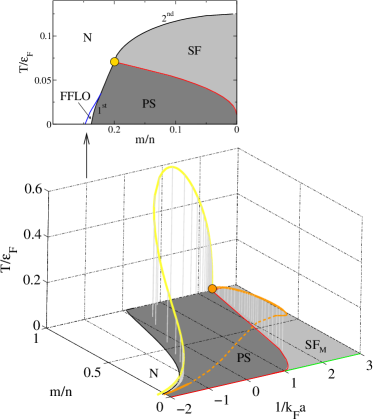
Figure 2: Finite temperature phase diagram as a function of magnetisation $m/n$ and interaction $1/k_{F}a$. The plane at temperature $T=0$ is the phase diagram in Fig. 1. The yellow line represents the locus of tricritical points calculated in the mean-field approximation, while the orange tricritical line corresponds to mean-field theory plus pair fluctuations. The fluctuation correction breaks down in the unitarity regime $-1<1/k_{F}a<1$, and is thus shown as a dotted line. The slice at $1/k_{F}a=-1$ is based on a mean-field calculation and it shows the region of phase separation terminating in a tricritical point (yellow circle) at finite temperature, followed by a second-order phase transition from the superfluid to normal state. Note that the boundary between the FFLO and normal states (blue line) defines a small region of FFLO phase confined to the BCS side of the crossover, as explained in the text.

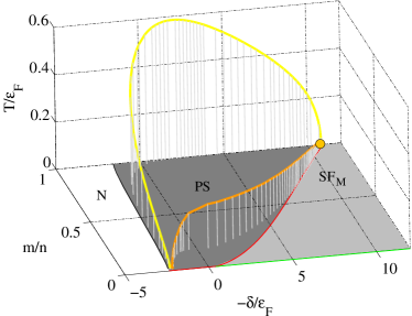
Figure 3: Finite temperature phase diagram for the two-channel model of a narrow Feshbach resonance, where the coupling between open and closed channels is weak: $\gamma=0.1$. The effective interaction is parameterised by the detuning $\delta/\varepsilon_{F}$. The colour scheme for tricritical lines is the same as in Fig. 2.

With this background, we now turn to the analysis of the fate of the tricritical point when temperature is finite, beginning with the mean-field description. It is well known that there exists a finite temperature tricritical point in the BCS limit $1/k_{F}a\to-\infty$, which is a natural consequence of having a first-order transition from the superfluid to normal state at $T=0$ and a second-order transition at $m=0$. First studied by Sarma in the context of superconductivity in the presence of a magnetic field Sarma (1963), the BCS tricritical point is located at $(T_{\textrm{crit}}/\Delta,h_{\textrm{crit}}/\Delta)=(0.3188,0.6061)$ Casalbuoni and Nardulli (2004), where $\Delta=\frac{8}{e^{2}}\varepsilon_{F}\exp\left[-\pi/2|k_{F}a|\right]$ (i.e. at weak coupling all energies scale with $\Delta$). This corresponds to a magnetisation $m=2\nu(\varepsilon_{F})h_{\textrm{crit}}$, where $\nu(\varepsilon_{F})=m_{f}^{3/2}\sqrt{\varepsilon_{F}}/\sqrt{2}\pi^{2}$ is the Fermi surface density of states. To investigate how the BCS tricritical point is related to the one at zero temperature, we must develop a perturbative expansion of Eq. (2) for small $\Delta$ and general $1/k_{F}a$. Doing so, one finds (Fig. 2) that the tricritical point at $m/n=1$ is connected to that in the BCS limit by a line of tricritical points that passes through a maximum somewhere in the ‘unitarity’ regime $-1<1/k_{F}a<1$. Moreover, for any given value of $1/k_{F}a\leq 2.368$, the $(T/\varepsilon_{F},m/n)$ phase diagram is highly reminiscent of the ³He-⁴He system, with $m/n$ playing the role of the fraction of ³He. This is not surprising, as the finite $m$ system corresponds in general to a mixture of bosonic pairs and fermionic quasiparticles. Note that even the gapped superfluid can be magnetised at finite temperature due to thermal excitation of quasiparticles. Of course, at $m=0$ the transition into the superfluid state is second order at any point in the BCS-BEC crossover.

It is interesting to examine how the FFLO phase fits in with the basic topology of the phase diagram. In the BCS limit, we already know that the point where the FFLO-normal phase boundary meets the normal-superfluid boundary asymptotes to the tricritical point Casalbuoni and Nardulli (2004). Assuming that the transition from the FFLO state to the normal state is second-order (although Ref. Combescot and Mora (2004) found it to be weakly first order, this will make a relatively small difference), and performing a mean-field analysis, we find that the FFLO point of intersection leaves the finite temperature tricritical point with increasing interaction (see Fig. 2), leading eventually to the extinction of the FFLO phase at $k_{F}a=-0.35$. Note that although this treatment is somewhat approximate, as we have taken the SF-FFLO boundary to be the same as the SF-N boundary in the absence of FFLO, the point of intersection will coincide with that derived from a complete mean-field analysis. Moreover, despite all our assumptions, we expect the detachment of the point of intersection from the tricritical point and the eventual disappearance of FFLO to be robust features, since in the BEC regime we essentially have a mixture of bosons and fermions.

The inclusion of the fluctuation contribution Eq. (3) is crucial for recovering the extreme BEC limit, where it is clear that the (second-order) transition temperature asymptotes to $T_{\mathrm{BEC}}(m)=T_{\mathrm{BEC}}\left(1-m/n\right)^{2/3}$ (with $T_{\mathrm{BEC}}\sim 0.218\varepsilon_{F}$), the ideal BEC temperature of a gas of bosons of density $n_{\downarrow}=(n-m)/2$ and mass $2m_{f}$. More importantly, we find that fluctuations shift the mean-field tricritical line to lower temperatures and magnetisations on the BEC side, while leaving the tricritical points on the BCS side largely unchanged, as expected. However, in a broad region around unitarity, we find that the approximation underlying Eq. (3) generally leads to non-monotonic behavior of $m(h)$, with $m(h>0)<0$ for small $h$. We interpret this behaviour as a breakdown of the NSR treatment, yielding an unphysical compressibility matrix $-\partial^{2}\Omega/\partial\mu_{\sigma}\partial\mu_{\sigma^{\prime}}$ that is not positive semi-definite.

To address this problem, we note that the NSR scheme is a controlled approximation when we introduce resonant scattering with a finite width, with the width being a small fraction of the Fermi energy Andreev et al. (2004). The simplest such description is provided by the two-channel model Timmermans et al. (2001); Holland et al. (2001). The two-channel description of scattering depends upon two parameters: a detuning $\delta/\varepsilon_{F}$ describing the distance from the resonance, and a width $\gamma$ of the resonance measured in units of the Fermi energy. The one-channel description is recovered in the $\gamma\to\infty$ limit, while the treatment of Gaussian fluctuations is essentially perturbative in $\gamma$, with $\Gamma^{-1}$ in Eq. (3) being replaced with $\frac{\mathbf{q}^{2}}{4m}-i\omega_{m}+\gamma\Gamma^{-1}(\mathbf{q},i\omega_{m})$, so in this case the NSR treatment is expected to be accurate. The resulting phase diagram is shown in Figure 3. The zero temperature phase diagram coincides with the result of Ref. Sheehy and Radzihovsky (2006). With fluctuations accounted for, and for sufficiently small $\gamma$, we now find a well-behaved line of tricritical points spanning the crossover region. We expect that the true phase boundary at $\gamma\to\infty$ is qualitatively similar.

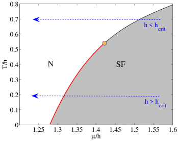
Figure 4: Phase diagram at $1/k_{F}a=0$ in the $\mu/h$-$T/h$ plane. The red and black lines are first- and second-order phase boundaries, respectively. The arrows at constant $T/h$ represent the trajectories followed when going from the centre to the edges of a trapped gas. The two trajectories correspond to two different magnetisations of the gas: one greater and one less than the tricritical point $h_{\textrm{crit}}$.

III Implications for experiment

We now discuss the consequences of our results for trapped gases studied in experiment. Modeling the trapped gas by the local density approximation (LDA), the spatial dependence of the density induced by the trapping potential $V({\mathbf{r}})$ is accounted for by a spatially-varying chemical potential $\mu({\mathbf{r}})=\mu-V({\mathbf{r}})$, with $h$ kept constant. In the $\mu/h$-$T/h$ plane, we thus move on a horizontal line (see Fig. 4). At sufficiently low temperatures, a trapped gas will consist of a superfluid core surrounded by the normal state. The transition between normal and superfluid states in the trap can be either second or first order, depending on whether $T/h$ is above or below the tricritical point. Moreover, as long as the temperature is non-zero, we can always find a sufficiently small $h$ so that $T/h$ lies above the tricritical point. This leads us to a key point: if a trapped gas at a given temperature and magnetisation has a first-order transition between its normal and superfluid phases, then we will always cross the tricritical point by decreasing the magnetisation at fixed temperature.

We emphasise that there are qualitative differences between first and second order transitions in a trap: the former yields a discontinuity in the density and magnetization at the phase interface, resulting in a form of phase separation as seen in recent experiments Zwierlein et al. (2006a); Partridge et al. (2006); Zwierlein et al. (2006b); Shin et al. (2006), while the latter possesses a density that varies smoothly in space. Therefore, the magnetisation and temperature at which a tricritical point is crossed should be detectable experimentally. In fact, a critical magnetisation for the onset of phase separation in a trap has been observed experimentally Partridge et al. (2006), and a calculation by Chevy supports the idea that this coincides with crossing a tricritical point Chevy (2006). In addition, the order of the transition will have an impact on experiments that use phase separation as a signature of superfluidity Zwierlein et al. (2006b).

The presence of a first-order transition in the trap can be even more pronounced if the density discontinuities result in a breakdown of LDA. Experiments on highly elongated traps already provide evidence for such a breakdown Partridge et al. (2006), and one requires the addition of surface energy terms at the phase interface to successfully model the trapped density profiles De Silva and Mueller (2006b).

An outstanding issue is the experimental detection of the gapless SF${}_{\textrm{M}}$ phase. While optically probing the momentum distribution of the minority species is one promising method for detecting SF${}_{\textrm{M}}$ Yi and Duan (2006b), another possibility is to study density correlations using, for example, shot noise experiments as suggested in Ref. Altman et al. (2004). A simple mean-field calculation gives (for the uniform system):

$$C_{\uparrow\downarrow}({\mathbf{k}_{1}},{\mathbf{k}_{2}}) \equiv\langle\hat{n}_{\uparrow}({\mathbf{k}_{1}})\hat{n}_{\downarrow}({\mathbf{k}_{2}})\rangle-\langle\hat{n}_{\uparrow}({\mathbf{k}_{1}})\rangle\langle\hat{n}_{\downarrow}({\mathbf{k}_{2}})\rangle$$

$$=\delta_{{\mathbf{k}_{1}},-{\mathbf{k}_{2}}}\frac{\Delta^{2}}{4E_{{\mathbf{k}_{1}}}^{2}}[1-f(E_{{\mathbf{k}_{1}}}+h)-f(E_{{\mathbf{k}_{1}}}-h)]^{2}$$

where $f(E)$ is the Fermi-Dirac distribution. At $T=0$, the result is a ‘hole’ in the correlation function for momenta less than the Fermi wavevector of the majority quasiparticles. Such a measurement would therefore constitute both a confirmation of the SF${}_{\textrm{M}}$ phase and a vivid demonstration of the blocking effect of quasiparticles on $\left(+\mathbf{k},-\mathbf{k}\right)$ pairing.

In conclusion, we have determined the structure of the finite temperature phase diagram of the two component Fermi gas, as a function of both interaction strength and population imbalance, finding a region of phase separation terminating in a tricritical point for general coupling in the BCS-BEC crossover. A secondary result of our work is the demonstration that the NSR scheme yields unphysical results in a broad region around unitarity. This is significant, as it is widely viewed as offering a smooth, albeit uncontrolled approximation throughout the crossover. We emphasize that there is no a priori reason to believe in the accuracy of the NSR scheme without introducing an additional parameter, as we have done here. The Ginzburg criterion governing the smallness of fluctuation corrections is satisfied in both the BCS limit where it takes the form $(T_{c}/\varepsilon_{F})^{2}\ll 1$, and in the BEC limit where $k_{F}a\ll 1$ is the relevant criterion. But at unitarity the shift in the transition temperature relative to the mean field value will be of order $\varepsilon_{F}$. At the same time the upper critical dimension at the tricritical point is three, so we may expect that our results there will be little changed.

Finally, we have argued that these tricritical points play an important role in experiments on trapped Fermi gases (see, also, the subsequent related work on trapped gases at unitarity by Gubbels et al. Gubbels et al. ). Indeed, a recent comprehensive study of the temperature dependence of the phase-separated state at unitarity has yielded experimental results consistent with the phase diagram outlined here Partridge et al. .