Fragmentation of Bose-Einstein Condensates

Abstract

We present the theory of bosonic systems with multiple condensates, unifying disparate models which are found in the literature, and discuss how degeneracies, interactions, and symmetries conspire to give rise to this unusual behavior. We show that as degeneracies multiply, so do the types of fragmentation, eventually leading to strongly correlated states with no trace of condensation.

I Bose-Einstein condensation, fragmented condensates, and strongly correlated states

Bose-Einstein condensation (BEC) is a very robust phenomenon. Because of Bose statistics, non-interacting bosons seek out the lowest single particle energy state and (below a critical temperature $T_{c}$) condense into it, even though many almost degenerate states may be nearby. At temperature $T=0$, the condensate contains all the particles in the system huang . Although this remarkable phenomenon was originally predicted by Einstein for non-interacting systems einstein , it became understood, starting with the work of F. London london , that it occurs in strongly interacting systems such as ⁴He. While interactions remove particles from the condensate into other states, the energy gain by macroscopically occupying the lowest energy state (or another state, such as a vortex) is sufficiently great that the interactions in a Bose condensed system manage only to deplete a fraction of the condensate, but not destroy it bogoliubov . This is the case for liquid ⁴He Penrose1956a as well as dilute gases of bosonic alkali atoms boseatoms .

In certain situations, however, a system does not condense into a single condensate nsj ; Nozieres1995a ; Wilkin1998a ; girardeau ; Koashi ; Ho1999a ; castin ; peth ; Rokhsar1998a ; spekkens ; jav ; dukelsky . In this paper we explore the physics of condensation when the ground state can contain several condensates – situations of fragmented condensation. This possibility arises naturally from the very concept of BEC – i.e., that the non-degenerate ground state of a single particle Hamiltonian $h_{0}$ is macroscopically occupied. How, instead, does condensation take place when the ground state of $h_{0}$ is degenerate, with two or more states competing simultaneously for condensation? What happens if the ground state degeneracy $G$ is not just of order unity, but of order $N$, the number of particles? And what happens if $G$ becomes much greater than $N$, or even approaches infinity? How do the bosons distribute themselves in these competing levels? In all these cases, interaction effects play an important role in determining the structure of the many-body ground state. Different types of interactions produce different fluctuations (such as those of phase, number, or spin) and lead to different classes of ground states.

Exact degeneracy is difficult to achieve, since small external fields or weak tunneling effects are generically present. Such energy-splitting effects lead to a non-degenerate ground state and therefore favor the formation of a single condensate. Only when interaction effects dominate over energy splittings can a single condensate break up.

Considerations of the effect of ground state degeneracies are not merely theoretical exercises. Rather, such degenracies occur in a wide range of current experiments in cold atoms. The cases where the degeneracy $G$ is of order unity are related to bosons with internal degrees of freedom. Examples include a pseudospin-1/2 Bose gas made up, e.g., of two spin states $|F=1,m=-1\rangle$ and $|F=2,m=1\rangle$) of ⁸⁷Rb jilaspinexp , and a spin-1 or spin-2 Bose gas such as ²³Na or ⁸⁷Rb in an optical trap spinexperiments . In the former case, even though the two spin states of ⁸⁷Rb are separated by a hyperfine splitting of order GHz, they can be brought to near degeneracy, with $G=2$, by applying an external rf field. In the spin-1 Bose gas, the three spin states are degenerate at zero external magnetic field, and $G=3$. The case of $G\sim N^{1/2}$ is encountered in one dimensional geometries 1dexp , where the density of states has a power law singularity at low energies. The case of $G\sim N$ is realized for bosons in optical lattices mott with $G$ sites each having a few bosons; in the limit of zero tunneling, $G$ equivalent sites compete for bosons. The case $G>>N$ is realized in rotating Bose gases with very large angular momentum, $L$, in a transverse harmonic trap hall ; wg . As $L$ increases, the rotation frequency $\Omega$ of the atom cloud approaches the frequency of the transverse harmonic trap, $\omega_{T}$, causing the single particle states to organize into Landau orbitals, which become infinitely degenerate as $\Omega\to\omega_{T}$. The great diversity of phenomena in these experiments is a manifestation of the physics of Bose condensation for varying degrees of degeneracy.

As we shall see, when the degeneracy is low ($G\sim 1$), a single condensate can break up into $G$ condensates. Following Nozières nsj ; Nozieres1995a , we refer to such a state as a fragmented condensate (define more precisely below). We caution, however, that there are many sorts of fragmented states. Even degeneracy as small as $G=2$ can give rise to fragmented condensates with distinct properties which depend on whether interaction effects favor phase or number fluctuations. System with larger degeneracies usually have a larger number of relevant interaction parameters and are more easily influenced by external fields. As a result, they have a greater variety of fragmented states. For degeneracies $G$ comparable to or much greater than the particle number, the system does not have enough particles to establish separate condensates. Instead, interactions effects tend to distribute bosons among different degenerate single particle states in a coherent way, establishing correlations between them. In such strongly correlated systems, interaction effects obliterate all traces of a conventional singly condensed state.

We stress at the outset that while interaction effects can cause fragmentation in the presence of degenerate single particle states, the presence of near degeneracies does not force the condensate to fragment. In many cases the ground state for a macroscopic Bose system is a conventional single condensate. Creating a fragmented state typically requires carefully tuning the parameters of the system, and whether such a state can occur in practice is very much dependent on the system. In optical lattices and double well systems, where the tunneling between wells can be tuned arbitrarily finely, a fragmented state can easily be achieved. Yet in other systems such as a spin-1 Bose gas in a single trap, or a rotating Bose gas, the parameter range allowing the existence of fragmented states scales like $1/N$, making it difficult to realize these ground states unless the number of particles is reduced to $\sim 10^{3}$ or fewer.

In this paper, we focus on fragmentation in the ground state of Bose systems. We consider a number of canonical examples (double-well systems, spin-1 Bose gases, and rotating Bose gases), which have increasing degeneracy in the single particle Hamiltonian. These examples illustrate the origin of fragmentation, the variety of fragmented states, and their key properties. We will not discuss here fragmentation in optical lattices or in dynamical processes, for they are a sufficiently large subject to require separate discussions. To begin, we first define condensate fragmentation more precisely, and the discuss general properties of certain classes of fragmented states.

II Definitions of condensation and fragmentation

The concept of Bose-Einstein condensation was generalized to interacting systems by Penrose and OnsagerPenrose1951a ; Penrose1956a in the 1950s, by defining condensation in terms of the single particle density matrix,

$$\rho^{(1)}({\bf r},{\bf r}^{\prime})=\langle\psi^{\dagger}({\bf r^{\prime}})\psi({\bf r})\rangle,$$ (1)

where $\psi^{\dagger}({\bf r})$ creates a scalar boson at position ${\bf r}$, and $\langle\rangle$ is the thermal average at temperature $T$. Since $\rho^{(1)}$ is a Hermitian matrix with indices ${\bf r}$ and ${\bf r^{\prime}}$, it can be diagonalized as,

$$\rho^{(1)}({\bf r},{\bf r}^{\prime})=\sum_{i}N_{i}(T)f_{i}({\bf r}^{\prime})^{\ast}f_{i}({\bf r}),$$ (2)

where the $N_{i}(T)$ are the eigenvalues and $f_{i}({\bf r})$ the orthonormal eigenfunctions of $\rho^{(1)}$; $\int f^{\ast}_{i}({\bf r})f_{j}({\bf r})=\delta_{ij}$. Setting ${\bf r}={\bf r}^{\prime}$ and integrating over ${\bf r}$ we have $\sum_{i}N_{i}(T)=N$, where $N$ is the number of particles. We label the eigenvalues in descending order, i.e., $N_{0}\geq N_{1}\geq N_{2}\geq\cdots$. Equation (2) implies that if one measures the number of bosons in the single particle state $f_{i}$, one finds $N_{i}$. This does not mean that the wavefunction of the many particle interacting system is a product of such single particle eigenstates. Unless there are special reasons (such as strict symmetry constraints, e.g., translational invariance), the eigenfunctions $\{f_{i}\}$ need not be the same as the single particle eigenstates $\{u_{i}\}$ of the single particle Hamiltonian of the non-interacting system. Two relevant examples are a homogeneous system of particles in free space, and a system in a harmonic trap. In the former case, where the momentum ${\bf k}$ is a good quantum number, we have $i={\bf k}$, and $\{f_{i}\}$ and $\{u_{i}\}$ are the same plane-wave momentum eigenstates. In an inhomogeneous trapped system, there is no simple relation between the $\{f_{i}\}$ and the $\{u_{j}\}$ dubois .

The usual situation of Bose condensation corresponds to the one eigenvalue $N_{0}$ being of order $N$, while other eigenvalues are of order unity, i.e.,

$${\rm BEC:}\,\,\,\,\,\,\,\,\,\,\rho^{(1)}({\bf r},{\bf r}^{\prime}) = N_{0}(T)f_{0}({\bf r}^{\prime})^{*}f_{0}({\bf r})+\cdots$$ (3)

$$\equiv \Psi^{(0)*}({\bf r}^{\prime})\Psi^{(0)}({\bf r})+\cdots\,,$$ (4)

or simply

$$\rho^{(1)}=N_{0}|\Psi^{(0)}\rangle\langle\Psi^{(0)}|+\cdots\,,$$ (5)

where $\Psi^{(0)}({\bf r})\equiv\sqrt{N_{0}}f_{0}({\bf r})$, and $(\cdots)$ denotes terms with eigenvalues $N_{i}\sim{\cal O}(1)$. Since the macroscopic term in Eq. (4) is identical to the density matrix of the pure single particle quantum state, $|\Psi^{(0)}\rangle$, the function $\Psi^{(0)}({\bf r})$ is often referred to as the “macroscopic wavefunction” of the system. Systems in which $\rho^{(1)}$ has only one macroscopic eigenvalue, Eq. (4), have single condensates. The advantage of the Penrose-Onsager characterization of BEC, Eq. (4), is that it applies to both interacting and non-interacting systems, since it makes no reference to dynamics. Penrose and Onsager also demonstrated the remarkable fact that Eq. (4) holds for a Jastrow function, which is a reasonable approximation to the ground state of a system of hard core bosons, therefore substantiating Eq. (4) as a general property of interacting Bose systems.

The Penrose-Onsager characterization can be easily generalized to bosons with internal degrees of freedom, labeled by an index $\mu$. With field operator $\psi^{\dagger}_{\mu}({\bf r})$, the single particle density matrix is

$$\rho^{(1)}({\bf r,\mu};{\bf r}^{\prime},\mu^{\prime}) = \Psi^{(0)*}_{\mu^{\prime}}({\bf r}^{\prime})\Psi^{(0)}_{\mu}({\bf r})+\cdots\,.$$ (6)

In a conventional noncondensed system, such as a zero temperature gas of non-interacting fermions, or a high temperature gas of bosons, all the occupation numbers are small: $N_{i}\sim{\cal O}(N^{0})$. A conventional singly condensed system has one large eigenvalue $N_{0}\sim{\cal O}(N)$, with all other eigenvalues small, $N_{i>0}\sim{\cal O}(N^{0})$. A fragmented system has $q>1$ large eigenvalues, $N_{i<q}\sim{\cal O}(N^{1})$. There is clearly a range of other possiblilites such as having an extremely large number $q\sim{\cal O}(N^{1/2})$ eigenvalues, each of which are of size $N_{i<q}\sim{\cal O}(N^{1/2})$. This latter case occurs in an interacting system of one dimensional bosons, and is associated with a phase incoherent quasicondensate lowd ; 1dexp .

II.1 Simple example of fragmentation and its relation with coherent states

Before examining the origin of fragmentation in detail, let us consider a basic example of fragmentation – the Nozières model Nozieres1995a . Consider a system of $N$ bosons each of which have available two internal states; 1 and 2. As we consider in detail later, this model can also be used to describe atoms in a double well potential. The Hamiltonian of Nozières’ model consists solely of an interaction between atoms in the two spin states,

$$H = \frac{g}{2}a^{\dagger}_{1}a^{\dagger}_{2}a_{2}a_{1}=\frac{g}{2}n_{1}n_{2},$$ (7)

where the $a^{\dagger}_{i}$ create bosons in state $i=1,2$, and $n_{i}=a^{\dagger}_{i}a_{i}$ is the number of particles in $i$. The interaction between the particles can be either repulsive ($g>0$) or attractive ($g<0$). The eigenstates have a definite number of particles in each well $|N_{1},N_{2}\rangle$, with $N=N_{1}+N_{2}$, and energy

$$E=\frac{g}{2}N_{1}N_{2}.$$ (8)

Clearly, for $g>0$, the ground state is two-fold degenerate, with $N_{1}=N,N_{2}=0$, or $N_{1}=0,N_{2}=N$; these states have single condensates, whose density matrices have eigenvalues 0 and $N$. On the other hand, for $g<0$, the state with $N_{1}=N_{2}=N/2\,$ has lowest energy. This Fock-state,

$$|F\rangle=\frac{a^{\dagger N/2}_{1}a^{\dagger N/2}_{2}}{(N/2)!}|0\rangle,$$ (9)

has a fragmented condensate; the corresponding single particle density matrix,

$$\rho^{(1)}=\langle a^{\dagger}_{\mu}a_{\nu}\rangle=\frac{N}{2}\left(\begin{array}[]{cc}1&0\\ 0&1\end{array}\right),$$ (10)

has two macroscopic eigenvalues.

One can contrast this fragmented state to the coherent state

$$|\phi_{N}\rangle=\frac{1}{\sqrt{2^{N}N!}}\left(e^{-i\phi/2}a^{\dagger}_{1}+e^{i\phi/2}a^{\dagger}_{2}\right)^{N}|0\rangle$$ (11)

in which $N$ bosons are condensed into the single particle state $(e^{-i\phi/2}a^{\dagger}_{1}+e^{i\phi/2}a^{\dagger}_{2})/\sqrt{2}$. The coherent state is an example of a single condensate, where the single particle density matrix, $\rho^{(1)}=\langle a^{\dagger}_{\mu}a_{\nu}\rangle$, is

$$\rho^{(1)} = \frac{N}{2}\left(\begin{array}[]{cc}1&e^{i\phi}\\ e^{-i\phi}&1\end{array}\right)$$ (14)

$$= \frac{N}{2}\left(\begin{array}[]{c}e^{-i\phi/2}\\ e^{i\phi/2}\end{array}\right)^{\ast}\begin{array}[]{cc}(e^{-i\phi/2}&e^{i\phi/2})\\ &\end{array}.$$ (19)

The difference between Eqs. (19) and (10) is the absence of the off-diagonal term $\langle a^{\dagger}_{1}a_{2}\rangle$ in the latter, which represents the loss of phase coherence in state (pseudospin) space.

II.2 Relation between Fock and coherent states

The Fock state (9) is an average over all coherent phase states $|\phi_{N}\rangle$, as we see from the relation,

$$|F\rangle = \frac{2^{N/2}}{\sqrt{N!}}\left(N/2\right)!\int^{\pi}_{-\pi}\frac{{\rm d}\phi}{2\pi}|\phi_{N}\rangle$$ (20)

$$\approx \left(\frac{\pi N}{2}\right)^{1/4}\int^{\pi}_{-\pi}\frac{{\rm d}\phi}{2\pi}|\phi_{N}\rangle;$$ (21)

the latter relation holds for $N>>1$. As we discuss in the next section, this connection is very useful for understanding the origin of various ground states. An important implication of this relation is that for a macroscopic system, the expectation value of any $p$-body operator, $\hat{O_{p}}\sim a^{\dagger}_{\mu_{1}}a^{\dagger}_{\mu_{2}}\dots a^{\dagger}_{\mu_{p}}a_{\nu_{p}}\dots a_{\nu_{2}}a_{\nu_{1}}$, in the Fock state is indistinguishable from that in an ensemble of coherent phase states $|\phi\rangle$, as long as $p\ll N$,

$$\langle F|\hat{O_{p}}|F\rangle=\int^{\pi}_{-\pi}\frac{{\rm d}\phi}{2\pi}\,\langle\phi_{N}|\hat{O_{p}}|\phi_{N}\rangle.$$ (22)

This equation, which we shall prove momentarily, shows that by measuring quantities associated with few body operators, one cannot distinguish a Fock state from an ensemble of coherent states with random phases Javmeasure ; castindalibard . An illustration of this effect is the interference of two condensates initially well separated from each other. Prior to any measurement process, the system is in a Fock state, Eq.(9), since there is no phase relation between the two condensates. Experimentally, in any single shot measurement (a photo of the interfering region), one finds an interference pattern consisting of parallel fringes whose location is specified by a phase $\phi$, as if the two far away condensates actually had a well defined relative phase with this value mitinterference . The value of $\phi$, however, varies randomly from shot to shot, so that if one averages over all the measurements, the interference fringes average out, as described simply by Eq. (22) puzzle .

To prove Eq. (22), we use Eq. (21) to write,

$$\langle F|\hat{O_{p}}|F\rangle=\sqrt{\frac{\pi N}{2}}\int^{\pi}_{-\pi}\frac{{\rm d}\phi^{\prime}}{2\pi}\frac{{\rm d}\phi}{2\pi}\,\langle\phi^{\prime}_{N}|\hat{O_{p}}|\phi_{N}\rangle;$$ (23)

it is then sufficient to show that $\langle\phi^{\prime}_{N}|\hat{O}_{p}|\phi_{N}\rangle$ vanishes unless the phases $\phi$ and $\phi^{\prime}$ are very close to each other. We note that

$$\langle\phi^{\prime}_{N}|\phi_{N}\rangle =\cos^{N}\left((\phi-\phi^{\prime})/2\right)\approx e^{-N(\phi-\phi^{\prime})^{2}/8}$$ (24)

$$\approx\sqrt{8\pi/N}\delta(\phi-\phi^{\prime}),$$

for $N>>1$. For $p$-body operators of the form $\hat{O}_{p}={a^{\dagger}_{1}}^{q^{\prime}}{a^{\dagger}_{2}}^{p-q^{\prime}}{a_{2}}^{p-q}{a_{1}}^{q}$,

$$\langle\phi^{\prime}_{N}|\hat{O}_{p}|\phi_{N}\rangle =$$ (25)

$$\frac{N!}{2^{p}(N-p)!}e^{i[\phi(p/2-q)-\phi^{\prime}(p/2-q^{\prime})]}\langle\phi^{\prime}_{N-p}|\phi_{N-p}\rangle.$$

For $N>>p$, we see from Eq. (24) that $\langle\phi^{\prime}_{N}|\hat{O}_{p}|\phi_{N}\rangle=\sqrt{8\pi/N}\langle\phi_{N}|\hat{O}_{p}|\phi_{N}\rangle\delta(\phi-\phi^{\prime})+{\cal O}(1/N)$, from which Eq. (22) follows.

III Characteristic examples of fragmentation

We now develop three different examples that illustrate the origin of fragmentation. These examples are chosen to illustrate the increasingly complex behavior of fragmentation when the number of degenerate single particle states increases.

III.1 Scalar bosons in double well

After the model of sec. II.1, the simplest model with a fragmented ground state is that of bosons in a double well potential with tunneling between the wells. Unlike in the previous example, this model produces two distinct types of fragmented states. We label the wells by $i=1,2$; we assume that there is only one relevant state in each well, and that particles within a given well have an interaction, $U$, which can be either repulsive ($U>0$) or attractive ($U<0$). We take the Hamiltonian to be

$$H=-t(a_{1}^{\dagger}a_{2}+a_{2}^{\dagger}a_{1})+\frac{U}{2}\left[n_{1}(n_{1}-1)+n_{2}(n_{2}-1)\right],$$ (26)

where the $a^{\dagger}_{i}$ creates a boson in well $i$, and $n_{i}=a^{\dagger}_{i}a_{i}$ is the number of particles in well $i$. The first term describes tunneling between the wells via a tunneling matrix element $t$ (which we assume to be real and positive). The form $Un_{i}(n_{i}-1)/2=Ua^{\dagger}_{i}a^{\dagger}_{i}a_{i}a_{i}/2$ is the usual contact interaction $(g/2)\int\psi^{\dagger}\psi^{\dagger}\psi\psi$ reduced to the single mode in each well. For fixed number of particles $n_{1}+n_{2}=N$, the interaction term can be written simply as

$$\hat{U}=\frac{U}{4}\left[\left(n_{1}-n_{2}\right)^{2}+N^{2}-2N\right]$$ (27)

This model, simple as it is, has wide applicability to many physical situations: atoms in a double well potential dwexp , internal hyperfine states coupled by electromagnetic fields jilaspinexp ; spinexperiments , atoms in a rotating toroidal trap uedaleggett , or wave packets in an optical lattice muellerswallowtails .

In solving this model it is useful to write Eq. (26) in the Wigner-Schwinger pseudospin representation lqm . We introduce the operators

$$J_{x} = (a^{\dagger}_{1}a_{2}+a^{\dagger}_{2}a_{1})/2,\,\,\,\,\,J_{y}=(a^{\dagger}_{1}a_{2}-a^{\dagger}_{2}a_{1})/2i,$$ (28)

$$J_{z}=(a^{\dagger}_{1}a_{1}-a^{\dagger}_{2}a_{2})/2,$$

which obey the angular momentum commutation relation $[J_{i},J_{j}]=i\epsilon_{ijk}J_{k}$, $i=x,y,z$, and satisfy

$${\bf J}^{2}=J_{x}^{2}+J_{y}^{2}+J_{z}^{2}=\frac{N}{2}\left(\frac{N}{2}+1\right).$$ (29)

The Hamiltonian (26) can be written in terms of ${\bf J}$ as

$$H=-2tJ_{x}+U(J_{z}^{2}+{\bf J}^{2}-N).$$ (30)

III.1.1 Mean-field solution

As we shall see, the Hamiltonian (26) can be solved exactly. Nonetheless, the mean-field solutions illustrate much of the physics of the true ground state. They also allow one to see the kind of fluctuations about the mean-field state that lead to condensate fragmentation.

The mean-field states are of the form of (pseudo)spinor condensates

$$|\theta,\phi\rangle=\frac{1}{\sqrt{N!}}(ua^{\dagger}_{1}+va^{\dagger}_{2})^{N}|0\rangle,$$ (31)

where $u=e^{-i\phi/2}\cos(\theta/2)$ and $v=e^{i\phi/2}\sin(\theta/2)$. The matrix elements of the density matrix in this state are $\langle a^{\dagger}_{1}a_{1}\rangle=\langle n_{1}\rangle=N\cos^{2}(\theta/2)$, $\langle a^{\dagger}_{2}a_{2}\rangle=\langle n_{2}\rangle=N\sin^{2}(\theta/2)$, and $\langle a^{\dagger}_{1}a_{2}\rangle=N\sin(\theta/2)\cos(\theta/2)e^{i\phi}$. The angles $\theta$ and $\phi$ therefore characterize the density and phase difference between the bosons in the two wells. In the pseudospin language, the state (31) describes a ferromagnet with total spin, $\langle{\bf J}\rangle=(N/2)\hat{\bf n}$, where $\hat{\bf n}=(\sin\theta\cos\phi,\sin\theta\sin\phi,\cos\theta)$ is the unit vector with polar angles $(\theta,\phi)$. According to Eq. (30), its energy is

$$E(\theta,\phi) = \langle\theta,\phi|H|\theta,\phi\rangle$$

$$= -tN\cos\phi\sin\theta+U\left(\frac{N^{2}}{4}(\cos^{2}\theta+1)-\frac{N}{2}\right).$$

For a repulsive interaction, $U>0$, $E(\theta,\phi)$ is minimum at $\phi=0$, $\theta=\pi/2$; or $\hat{\bf n}=\hat{\bf x}$. The mean-field approach therefore selects the non-interacting ground state $|C\rangle=(a^{\dagger}_{1}+a^{\dagger}_{2})^{N}|0\rangle/\sqrt{2^{N}N!}=|\hat{\bf x}\rangle$ as optimal. Condensates in the neighborhood of $|C\rangle$ have energy

$$E(\pi/2+\epsilon,\phi)=E(\pi/2,0)+\frac{1}{2}tN\phi^{2}+\frac{N}{4}(2t+UN)\epsilon^{2}+\dots.$$ (33)

From this result one can begin to see problems with the mean-field solution: as $t\to 0$ with fixed $U$, the energy of phase fluctuations ($\phi$) vanishes; therefore quantum fluctuations begin to mix in many nearly degenerate phase states, $|\pi/2,\phi\rangle$.

The mean-field solution for attractive $U$ is very different from that of repulsive $U$. The solution depends on whether $|U|N<2t$ or $|U|N>2t$. In the former case, $|C\rangle$ is locally stable since the energy of fluctuations, described by Eq. (33), remain positive definite. However, the stiffness constant for density fluctuations ($\epsilon$) is lower than that for phase fluctuations ($\phi$). Thus, as $|U|$ increases, density fluctuations become dominant. Note, however, that the condition $|U|N<2t$ only occurs for a bounded number of particles, and under ordinary circumstances is not expected to be achievable in macroscopic systems. On the other hand, when $|U|N>2t$, we see from Eq. (III.1.1) that the optimal states satisfy $\sin\theta=2t/|U|N$. There are two degenerate solutions: $\theta=\theta_{0}=\arcsin(2t/|U|N)$ and $\pi-\theta_{0}$. For $|UN|/2t>>1$, these two states approach $\sim a^{\dagger N}_{1}|0\rangle/\sqrt{N!}$ and $\sim a^{\dagger N}_{2}|0\rangle/\sqrt{N!}$, corresponding to all particles being in well 1 or 2 respectively.

III.1.2 Exact ground states

We now construct the exact ground state of the Hamiltonian, (26), and see how interactions can cause condensate fragmentation. At the same time, we can see how different types of interaction cause different types of fragmented states.

Non-interacting case: Let us first consider the simplest case of non-interacting bosons, with Hamiltonian $H=-t(a^{\dagger}_{1}a_{2}+{\rm h.c.})$. The single particle eigenstates are the symmetric state $(a_{1}+a_{2})/\sqrt{2}$ and antisymmetric state $(a_{1}-a_{2})/\sqrt{2}$ with energy $-t$ and $t$ respectively. For a system of $N$ bosons, the ground state is

$$|C\rangle=\frac{1}{\sqrt{2^{N}N!}}(a^{\dagger}_{1}+a^{\dagger}_{2})^{N}|0\rangle$$ (34)

with energy $-tN$. The single particle density matrix of this state is

$$\langle a^{\dagger}_{\mu}a_{\nu}\rangle_{{}_{C}}=\frac{N}{2}\left(\begin{array}[]{cc}1&1\\ 1&1\end{array}\right)=N\left(\begin{array}[]{c}\frac{1}{\sqrt{2}}\\ \frac{1}{\sqrt{2}}\end{array}\right)\begin{array}[]{cc}\left(\frac{1}{\sqrt{2}}\right.,&\left.\frac{1}{\sqrt{2}}\right),\\ &\end{array}$$ (35)

which has a single macroscopic eigenvalue $\lambda=N$. The ground state is therefore a single condensate with condensate wavefunction $\zeta^{T}_{\mu}=\sqrt{N/2}(1,1)$ (the superscript “$T$” stands for transpose).

Since the ground state $|C\rangle$ is a linear combination of number states $|n_{1},n_{2}\rangle=a^{\dagger n_{1}}_{1}a^{\dagger n_{2}}_{2}|0\rangle/\sqrt{n_{1}!n_{2}!}$, the number of particles in each well fluctuates.

We calculate the number fluctuations of the coherent state $|C\rangle$ by writing it in the number basis. For even $N$, we have

$$|C\rangle=\sum_{\ell=-N/2}^{N/2}\Psi^{(0)}_{\ell}|\ell\rangle,$$ (36)

where $|\ell\rangle\equiv|\frac{N}{2}+\ell,\frac{N}{2}-\ell\rangle$, and

$$\Psi^{(0)}_{\ell}=\left(\frac{N!}{2^{N}(\frac{1}{2}N+\ell)!(\frac{1}{2}N-\ell)!}\right)^{1/2}\approx\frac{e^{-\ell^{2}/N}}{(\pi N/2)^{1/4}}.$$ (37)

The number fluctuations are then

$$\langle\Delta N_{1}^{2}\rangle=\langle(N_{1}-\langle N_{1}\rangle)^{2}\rangle\approx\int{\rm d}\ell\,\frac{\ell^{2}e^{-2\ell^{2}/N}}{\sqrt{\pi N/2}}=N/4,$$ (38)

which, despite the approximations made in this derivation, coincides with the exact result.

Interacting Case: The many-body physics of this double well system is completely tractable. While one can calculate the properties the ground state numerically to arbitrary accuracy, we derive below all the essential features of the ground state by studying the effect of interactions on the non-interacting ground state, i.e., the coherent state $|C\rangle$. We shall see that depending on whether the interactions are repulsive or attractive, the coherent state can be turned into one of two distinct fragmented states: a ‘Fock-like’ state or a ‘Schrödinger cat-like’ state.

We first look at the Schrödinger equation of this system. Writing the ground state in the number basis,

$$|\Psi\rangle=\sum_{\ell=-N/2}^{N/2}\Psi_{\ell}|\ell\rangle,$$ (39)

we can write the Schrödinger equation, $H|\Psi\rangle=E|\Psi\rangle$, where $H$ is given by Eq. (26), as

$$E\Psi_{\ell}=-t_{\ell+1}\Psi_{\ell+1}-t_{\ell}\Psi_{\ell-1}+U\ell^{2}\Psi_{\ell},$$ (40)

$$t_{\ell}=t\sqrt{(N/2+\ell)(N/2-\ell+1)}.$$ (41)

The many-body problem then reduces to a one-dimensional tight binding model in a harmonic potential. The special feature of this model is that the tunneling matrix element $t_{\ell}$ is highly non-uniform spintrans : $t_{\ell}\sim N/2$ for $\ell\approx 0$, and $t_{\ell}\sim\sqrt{N/2}$ for $\ell\approx\pm N/2$. This non-uniformity is a consequence of bosonic enhancement, $a^{\dagger}|N\rangle=\sqrt{N+1}|N+1\rangle$ and $a|N\rangle=\sqrt{N}|N-1\rangle$, which increases the matrix element by a factor of $\sqrt{N}$ when removing a particle from a system with $N$ bosons. As a result, $\langle\ell+1|a^{\dagger}_{1}a_{2}|\ell\rangle$ is maximum when both wells have equal number of bosons (i.e., $\ell\sim 0$), and drops rapidly when the difference in boson numbers between the wells begins to increase, (i.e., $\ell>>1$). A consequence is that hopping favors wavefunctions $\Psi_{\ell}$ having large amplitudes near $\ell=0$. For example, in the non-interacting case the wavefunction, Eq. (37), is a sharply peaked Gaussian at $\ell=0$.

The interaction term, $U(n_{1}-n_{2})^{2}/4$, leads to a harmonic potential in Eq. (40). Repulsive interactions $(U>0)$ suppress number fluctuations, meaning that the Gaussian distribution [Eq. (37)] of the coherent state will be squeezed into an even narrower distribution. In the limit of zero number fluctuation,

$$\langle(\Delta n_{1})^{2}\rangle=\langle(\Delta n_{2})^{2}\rangle=0,$$ (42)

the system becomes the Fock state

$$|F\rangle=\frac{a^{\dagger N/2}_{1}a^{\dagger N/2}_{2}}{(N/2)!}|0\rangle,$$ (43)

which is clearly fragmented, since it is made up of two independent condensates. This fragmentation shows up clearly in the single particle density matrix,

$$\langle a^{\dagger}_{\mu}a_{\nu}\rangle = \frac{N}{2}\left(\begin{array}[]{cc}1&0\\ 0&1\end{array}\right)$$ (46)

$$= \frac{N}{2}\left(\begin{array}[]{c}1\\ 0\end{array}\right)\left(\begin{array}[]{cc}1&0\end{array}\right)+\frac{N}{2}\left(\begin{array}[]{c}0\\ 1\end{array}\right)\left(\begin{array}[]{cc}0&1\end{array}\right),$$ (53)

which has two macroscopic eigenvalues, corresponding to independent condensation in each well. The evolution from the coherent state $|C\rangle$ to the Fock state $|F\rangle$ can be captured by the family of states

$$\Psi_{\ell}(\sigma)=\frac{e^{-\ell^{2}/\sigma^{2}}}{(\pi\sigma^{2}/2)^{1/4}}.$$ (54)

As $1/\sigma^{2}$ varies from $1/N$ to much greater than unity, the initial coherent state $|C\rangle$ becomes more and more Fock-like. Indeed, exact numerical solution of Eq. (40) shows that Eq. (54) is an accurate description of the evolution from a coherent state towards a Fock state. During the collapsing process when the wavefunction $\Psi_{\ell}$ still extends over many number states (but fewer than $(N/2)^{-1/2}$), one can take the continuum limit of Eq. (40), which reduces to the equation for a particle in a harmonic oscillator potential. From its Gaussian ground state wavefunction, we extract $\sigma^{-2}=(2/N)(1+UN/t)^{1/2}$.

Using this continuum approximation, we calculate the off-diagonal matrix element,

$$\langle a^{\dagger}_{1}a_{2}\rangle = \sum_{\ell}\sqrt{(N/2-\ell)(N/2+\ell+1)}\Psi_{\ell+1}\Psi_{\ell}$$ (55)

$$\approx (N/2)e^{-1/(2\sigma^{2})},$$ (56)

which leads to a single particle density matrix

$$\langle a^{\dagger}_{\mu}a_{\nu}\rangle=\frac{N}{2}\left(\begin{array}[]{cc}1&e^{-1/2\sigma^{2}}\\ e^{-1/2\sigma^{2}}&1\end{array}\right).$$ (57)

The eigenvalues are $\lambda_{1}=\frac{N}{2}(1+e^{-1/\sigma^{2}})$, and $\lambda_{2}=\frac{N}{2}(1-e^{-1/\sigma^{2}})$. The relative number fluctuations are

$$\langle(\Delta n_{1})^{2}\rangle=\sigma^{2}/2.$$ (58)

As $1/\sigma^{2}$ varies from $1/N$ to a number much larger than unity, the eigenvalues $(\lambda_{1},\lambda_{2})$ varies from $(N,0)$ to $(N/2,N/2)$, and $\sqrt{\langle(\Delta n_{1})^{2}\rangle}$ varies from $\sqrt{N}$ to 0.

This transition of the coherent state into a Fock state, described by the family Eq. (54), is due to increasing phase fluctuations, as discussed in sec. III.1.1. The phase fluctuation effect can be seen by writing Eq. (54) in terms of phase states,

$$|\phi\rangle = \frac{1}{\sqrt{2^{N}N!}}\left(e^{i\phi/2}a^{\dagger}_{1}+e^{-i\phi/2}a^{\dagger}_{2}\right)^{N}|0\rangle$$ (59)

$$= \sum_{\ell}e^{i\phi\ell}\Psi^{(0)}_{\ell}|\ell\rangle,$$

where $\Psi_{\ell}^{(0)}$ are the coefficients given by Eq.(37). The family of q.(54) then becomes

$$|\Psi(\sigma)\rangle=\frac{(\pi\overline{\sigma}^{2})^{1/2}}{(\sigma^{2}/N)^{1/4}}\int^{\pi}_{-\pi}\frac{{\rm d}\phi}{2\pi}e^{-\overline{\sigma}^{2}\phi^{2}/4}|\phi\rangle$$ (60)

where $\overline{\sigma}^{-2}=\sigma^{-2}-N^{-1}$. As $\sigma^{-2}$ varies from $\sigma^{-2}\sim N^{-1}$ (coherent state) to $\sigma^{-2}>>1$, the Gaussian in Eq. (60) changes from a $\delta$-function, $\delta(\phi),$ to a uniform distribution, thereby driving the coherent state towards a Fock state.

Attractive Interaction: When $U<0$, the potential energy $U(n_{1}-n_{2})^{2}/4$ in Eq. (27) favors a large number difference between the two wells, in particular, the states $|\ell=N/2\rangle=|N,0\rangle$ and $|\ell=-N/2\rangle=|0,N\rangle$. It therefore acts in the opposite direction as hopping, which favors a Gaussian distribution of number states around $|\ell=0\rangle$. The effect of interaction is then to split the Gaussian peak of the coherence state Eq. (37) into two peaks, a process which can be described by the family of states HoCio ,

$$\Psi_{\ell}(a)=C\left(e^{-(\ell-a)^{2}/2\sigma^{\prime 2}}+e^{-(\ell+a)^{2}/2\sigma^{\prime 2}}\right)$$ (61)

where $2a$ is the separation between the peaks, $\sigma^{\prime}$ is the width of the peaks, and $C$ is the normalization constant. As $a$ varies from 0 toward $N/2$, and $\sigma^{\prime}$ shrinks at the same time from $1/\sqrt{N}$ to 0, the state $|\Psi(a)\rangle=\sum_{\ell}\Psi_{\ell}|\ell\rangle$ evolves from the coherent state $|C\rangle$ to a Schrödinger-cat state

$$|Cat\rangle=\frac{1}{\sqrt{2}}\left(|N,0\rangle+|0,N\rangle\right).$$ (62)

The Schrödinger-cat state is fragmented in the sense that its single particle density matrix has two large eigenvalues,

$$\langle a^{\dagger}_{\mu}a_{\nu}\rangle=\frac{N}{2}\left(\begin{array}[]{cc}1&0\\ 0&1\end{array}\right),$$ (63)

identical to that of Fock state. On the other hand, contrary to the Fock state, it has huge number fluctuations,

$$\langle(\Delta n_{1})^{2}\rangle=\langle(\Delta n_{2})^{2}\rangle=N^{2}/4.$$ (64)

Details of how $a$ and $\sigma^{\prime}$ depend on the ratio $U/t$ are found in HoCio , where it is also shown that the family Eq. (61) accurately represents the numerical solution of Eq. (40). This double-well example brings out the important point that fragmented condensates cannot be characterized by the single particle density matrix alone. Higher order correlation functions such as number fluctuations are needed. This example also shows how a coherent state can be brought into a Fock state (or Schrödinger-cat state) through the phase (or number) fluctuations caused by repulsive (or attractive) interaction.

III.2 Spin-1 Bose gas

The spin-1 Bose gas, which is only marginally more complicated, provides an excellent illustration of the role of symmetry in condensate fragmentation. Here the degeneracies that give rise to fragmentation are due to a symmetry: rotational invariance in spin space. We will see that in the presence of local antiferromagnetic interactions all low energy singly condensed states break this symmetry. The true ground state, which is a quantum superposition of all members of this degenerate manifold, is a fragmented condensate.

We consider a spin-1 Bose gas with $2N$ particles in the single mode approximation, where each spin state has the same spatial wavefunction. Several recent experiments have been carried out in this limit sengstock ; hirano ; Chapman (note that several of these experimental also explored regimes where the single mode approximation was not valid Saito ). For conceptual clarity we consider the extreme case where the trap is so deep that all particles reside in the lowest harmonic state, trivially leading to the single mode limit. In this extreme situation there are no particle fluctuations: the only relevant interaction is scattering between different spin states. We denote the creation operator of a boson with spin projection $\mu$ = (1,0,-1) in the lowest harmonic state by $a^{\dagger}_{\mu}$; the number of bosons with spin $\mu$ is $N_{\mu}=a^{\dagger}_{\mu}a_{\mu}$. The most general form of the scattering Hamiltonian which is rotational invariant in spin space is Ho

$$H=c{\bf S}^{2}$$ (65)

where ${\bf S}=\sum_{\mu\nu}a^{\dagger}_{\mu}{\bf S}_{\mu\nu}a_{\nu}$, with $S^{i}_{\mu\nu}$ the spin-1 matrices, ($i=x,y,z$), and $c$ the interaction constant. We consider the case $c>0$. More complicated Hamiltonians, with more interaction terms, are allowed for atoms with higher spins HoLan ; Ueda . The variety of fragmented states proliferate rapidly as the atomic spin increases.

To illustrate how condensate fragmentation is affected by external perturbations, we include the linear Zeeman effect, with Hamiltonian,

$$H_{Z}=-pS_{z}=-p(N_{1}-N_{-1}),$$ (66)

where $p$ is the Zeeman energy proportional to the external magnetic field $B$. To explain current experiments one also needs to include the quadratic Zeeman effect: the atomic energy levels of atoms are not linear in $B$ due to hyperfine interaction between electron spins and nuclear spins. We ignore these nonlinearities as they are irrelevant for describing fragmentation.

For later discussion, we also include a term of the form

$$H_{G}=\epsilon(a^{\dagger}_{1}a_{-1}+a^{\dagger}_{-1}a_{1}),$$ (67)

which mixes spin states $1$ and $-1$, where $\epsilon$ is a constant. Terms of this form can be generated by magnetic field gradients Ho1999a , in which case $\epsilon$ is proportional to the square of the field gradient. Since both $H$ and $H_{Z}$ conserve $S_{z}$, the density matrix $\langle a^{\dagger}_{\mu}a_{\nu}\rangle$ for the ground state is diagonal in the presence of these terms alone, and the system is generally fragmented unless the density matrix happens to have only one macroscopic eigenvalue. The effect of $H_{G}$ is to mix the 1 and -1 states, bringing the system into coherence, similar to the role of the tunneling term in the double well system.

III.2.1 Mean-field approach

Like the double well problem in the previous section, the Hamiltonian in Eq. (65) is exactly soluble. As previously, we first consider the mean-field solution so that we can relate the fragmented condensate to a linear combination of singly condensed states.

The general form of a singly condensed spinor Bose condensate is

$$|\zeta\rangle_{N}=\frac{1}{\sqrt{N!}}\left(\sum_{\mu}\zeta_{\mu}a^{\dagger}_{\mu}\right)^{N}|0\rangle,\,\,\,\,\,\,\,\,\sum_{\mu}|\zeta_{\mu}|^{2}=1.$$ (68)

Using the fact that $a_{\beta}a_{\nu}|\zeta\rangle_{N}=\sqrt{N(N-1)}\zeta_{\beta}\zeta_{\nu}|\zeta\rangle_{N-2}$, it is easy to see that the number fluctuations are $\langle N^{2}_{\nu}\rangle-\langle N_{\mu}\rangle^{2}=\langle N_{\nu}\rangle=N|\zeta_{\mu}|^{2}$. Writing the Hamiltonian as,

$$H={\bf S}_{\mu\nu}\cdot{\bf S}_{\alpha\beta}\,a^{\dagger}_{\mu}a^{\dagger}_{\alpha}a_{\beta}a_{\nu}+2\hat{N},$$ (69)

we have, up to terms ${\cal O}(N^{-1})$,

$$\langle H+H_{Z}\rangle_{|\zeta\rangle_{N}}=c\langle{\bf S}\rangle^{2}-p\langle S_{z}\rangle+2cN$$ (70)

where $\langle{\bf S}\rangle=N\sum_{\mu,\nu}\zeta^{\ast}_{\mu}{\bf S}_{\mu\nu}\zeta_{\nu}$. It is easy to see that Eq.(70) is minimized by

$$\zeta^{T}_{\phi}=e^{i\gamma}\left(e^{-i\phi}\sqrt{\frac{N_{1}}{N}},0,e^{i\phi}\sqrt{\frac{N_{-1}}{N}}\right),$$ (71)

where, as before, $T$ stands for transpose, $\phi$ is the relative phase between the 1 and $-1$ component, $N_{1}+N_{-1}=N$, and the difference $M=N_{1}-N_{-1}=\langle S_{z}\rangle$ is given by the nearest integer to $p/2c$. Note that $\langle S_{x}\rangle=\langle S_{y}\rangle=0$, and the entire family $\{\zeta_{\phi}\}$ is degenerate, reflecting the invariance of Eq. (70) under spin rotation about the $z$-axis. In the absence of a magnetic field, $p\rightarrow 0$, we have $\zeta^{T}_{\phi}\rightarrow e^{i\gamma}\left(e^{-i\phi},0,e^{i\phi}\right)/\sqrt{2}$. However, since Eq. (70) becomes fully rotationally invariant at zero field, any arbitrary rotation of the state $\left(1,0,1\right)/\sqrt{2}$ is also an optimal spinor condensate. The entire degenerate family (referred to as the “polar” family in literature) is given by

$$\zeta^{(0)}_{\phi}=e^{i\gamma}\left(\begin{array}[]{c}-\frac{1}{\sqrt{2}}e^{-i\phi}{\rm sin}\theta\\ {\rm cos}\theta\\ \frac{1}{\sqrt{2}}e^{i\phi}{\rm sin}\theta\end{array}\right),$$ (72)

with energy

$$\langle H\rangle_{\rm polar}=2cN.$$ (73)

Before discussing the exact ground states, we introduce the “Cartesian” operators

$$A_{x}=-\frac{a_{1}+a_{-1}}{\sqrt{2}},\,\,\,\,\,A_{y}=\frac{a_{1}-a_{-1}}{i\sqrt{2}},\,\,\,\,\,A_{z}=a_{0}.$$ (74)

The important properties of these operators is that that under a spin rotation $a_{\mu}\to U_{\mu\nu}a_{\nu}$, where $U={\rm exp}(-i\vec{\theta}\cdot{\bf S})$, ${\bf A}$ rotates like a Cartesian vector, i.e. $A_{i}\to R(\vec{\theta})_{ij}A_{j}$, where $R_{ij}(\vec{\theta})$ is a rotational matrix in Cartesian space ($xyz$). It is easily verified that $[A_{i},A^{\dagger}_{j}]=\delta_{ij}$, and

$${\bf S}=-i{\bf A}^{\dagger}\times{\bf A},\,\,\,\,\,\,\,\,N={\bf A}^{\dagger}\cdot{\bf A},$$ (75)

$$H=c\left[N^{2}-\Theta^{\dagger}\Theta\right],\,\,\,\,\,\,\,\,\,\,\,\Theta={\bf A}^{2}.$$ (76)

and the operator that creates a singlet pair is,

$$\Theta^{\dagger}={\bf A}^{\dagger 2}=-2a^{\dagger}_{1}a^{\dagger}_{-1}+a^{\dagger 2}_{0}.$$ (77)

The mean-field state Eq. (68) can now be written as

$$|\vec{\alpha}\rangle=\left(\vec{\alpha}\cdot{\bf A}^{\dagger}\right)^{N}|0\rangle/\sqrt{N!},\,\,\,\,\,\,\,\,\vec{\alpha}^{\ast}\cdot\vec{\alpha}=1.$$ (78)

which has average spin

$$\langle{\bf S}\rangle=-iN\vec{\alpha}^{\ast}\times\vec{\alpha}$$ (79)

The optimal mean-field state is determined by minimizing

$$\langle\vec{\alpha}|H|\vec{\alpha}\rangle=cN^{2}\left[1-|\vec{\alpha}\cdot\vec{\alpha}|^{2}\right]-ipN\hat{\bf z}\cdot\vec{\alpha}^{\ast}\times\vec{\alpha}.$$ (80)

In zero field ($p=0$), the optimal mean-field state is $\vec{\alpha}=\hat{\bf n}$, where $\hat{\bf n}$ is a real unit vector. The polar family mentioned above can now be conveniently represented by all possible directions of $\hat{\bf n}$, and the polar state in Eq. (72) corresponds to

$$|\hat{\bf n}\rangle=\frac{(\hat{\bf n}\cdot{\bf A}^{\dagger})^{N}}{\sqrt{N!}}|0\rangle.$$ (81)

III.2.2 Exact ground state in a uniform magnetic field:

In the absence of a magnetic field, $H=c{\bf S}^{2}$. Since $H$ is proportional to the angular momentum operator, the ground state for $C>0$ (with an even number of bosons $N$) is a singlet. The singlet state of a single mode spin-1 Bose gas is unique HoLan , and hence any manifestly rotationally invariant state must be the ground state. One can therefore obtain the ground state by forming singlet pairs, which for an even number of particles yields Koashi ; Law1998c ; Ho1999a

$$|S=0\rangle\propto({\bf A}^{\dagger}\cdot{\bf A}^{\dagger})^{N/2}|0\rangle.$$ (82)

Since this state is rotationally invariant, its single particle density matrix $\langle a^{\dagger}_{\mu}a_{\nu}\rangle$ is proportional to the identity matrix (Shur’s theorem). With the constraint $N=\sum_{\mu}a^{\dagger}_{\mu}a_{\mu}$, we then have

$$\langle a^{\dagger}_{\mu}a_{\nu}\rangle_{|S=o\rangle}=\frac{N}{3}\delta_{\mu\nu}$$ (83)

The condensate is therefore fragmented into three large pieces. The energy of the ground state is exactly zero, whereas that of the mean-field state is $2cN$ (as shown in Eq. (73)).

To relate the exact ground to the optimal mean-field state (the polar family $\{|\hat{\bf n}\rangle\}$), we note that

$$|S=0\rangle\propto\int\frac{{\rm d}\hat{\bf n}}{4\pi}\left(\hat{\bf n}\cdot{\bf A}^{\dagger}\right)^{N}|0\rangle,$$ (84)

i.e., the exact ground state is an average over the family of optimal mean field states. This is the analog of the symmetry averaging relation in Eq. (22). This averaging process represents the quantum fluctuations within the family of degenerate mean-field states; the effect of these fluctuations is to reduce the mean-field energy from $2cN$ to zero.

Next we consider the case of non-zero magnetic field $p\neq 0$. the Hamiltonian is $H+H_{Z}=c{\bf S}^{2}-pS_{z}$. The ground state is $|S,S_{z}=S\rangle$ or simply denoted as $|S,S\rangle$, where $S$ is an integer closest to $p/2c$. The state $|S,S\rangle$ can be easily obtained by changing a singlet pair into a triplet pair, and we have

$$|S,S\rangle={\cal D}a^{\dagger S}_{1}\left({\bf A}^{\dagger 2}\right)^{(N-S)/2}|0\rangle,$$ (85)

where ${\cal D}$ is a normalization constant, and Bose statistics require $S$ to be even if $N$ is even. Since the Hamiltonian $H+H_{Z}$ conserves $S_{z}$, the single particle density matrix remains diagonal, $\langle a^{\dagger}_{\mu}a_{\nu}\rangle=N_{\mu}\delta_{\mu\nu}$. As shown in Koashi ; Ho1999a , the eigenvalues $N_{\mu}$ have a very interesting behavior as a function of $S$, namely

$$N_{1}=\frac{N(S+1)+S(S+2)}{2S+3},$$ (86)

$$N_{-1}=\frac{(N-S)(S+1)}{2S+3},\,\,\,\,\,\,\,N_{0}=\frac{N-S}{2S+3}.$$ (87)

If $S$ is of order 1, all three eigenvalues, $N_{\pm 1},N_{0},$ are macroscopic. On the other hand, if $S$ becomes macroscopic, (i.e., $S/N$ is less than but of order 1), both $N_{1}$ and $N_{-1}$ remain macroscopic (with $N_{1}\rightarrow(N+S)/2$ and $N_{-1}\rightarrow(N-S)/2$) while $N_{0}$ becomes of order unity. This means as $S$ increases, the $S_{z}=0$ component is completely depleted. Although the system is still fragmented, the number of fragmented pieces is reduced from three to two, even for a tiny spin polarization. Further analysis Ho1999a shows that as one increases $S$, the fluctuations, $\langle\Delta N_{1}^{2}\rangle=\langle N_{1}^{2}\rangle-\langle N_{1}\rangle^{2}$, drop rapidly.

The reduction in the number of fragmented pieces mirrors the previously discussed reduction in the size of the space of degenerate mean-field states. In the absence of a magnetic field, polar states with arbitrary $\bf\hat{n}$ are degenerate, while a magnetic field in the $\bf\hat{z}$ direction favors those with $\bf\hat{n}$ pointing in the x-y plane.

To connect the exact polarized states to the mean-field states, we use the relation ${\bf A}^{\dagger 2}=-2a^{\dagger}_{1}a^{\dagger}_{-1}+a^{\dagger 2}_{0}$, Eq. (77), to write

$$({\bf A}^{\dagger 2})^{(N-S)/2}|0\rangle=\sum_{p=0}^{(N-S)/2}D_{p}|p,N-S-2p,p\rangle$$ (88)

where the exact form of $D_{p}$ is not important for our discussion. If we now act on $({\bf A}^{\dagger 2})^{(N-S)/2}|0\rangle$ by $a_{1}^{\dagger}$, the coefficients of the large $p$ states in Eq. (88) will be bosonically enhanced via $a^{\dagger}_{1}|N_{1}\rangle=\sqrt{(N_{1}+1)}|N_{1}+1\rangle$. Further acting on the same state by $a^{\dagger}_{1}$ eventually picks out the term with largest $p$, which is $|(N+S)/2,0,(N-S)/2\rangle$, in the sum Eq. (88). This process is equivalent to replacing $a^{\dagger S}_{1}(-2a^{\dagger}_{1}a^{\dagger}_{-1}+a^{\dagger 2}_{0})^{(N-S)/2}|0\rangle$ by $a^{\dagger S}_{1}(-2a^{\dagger}_{1}a^{\dagger}_{-1})^{(N-S)/2}|0\rangle$. We then have

$$|S,S\rangle \propto a^{\dagger S}_{1}({\bf A}^{\dagger 2})^{(N-S)/2}|0\rangle\approx a^{\dagger S}_{1}(-2a^{\dagger}_{1}a^{\dagger}_{-1})^{(N-S)/2}$$ (89)

$$\propto a^{\dagger(N+S)/2}_{1}a^{\dagger(N-S)/2}_{-1}|0\rangle.$$

From our previous analysis of the two-well system it is clear that this state is formed from an angular average of Eq. (71). The field gradient term (67) plays the role of tunneling in the two-well system and can drive the system from a fragmented to coherent state.

To complete the connection between these examples, we note that when the occupation of the $S_{z}=0$ state is negligible, we can set $a_{0}=0$, and only two spin states are required to describe the system. Under these conditions, the Hamiltonian for the spin 1 gas [Eqs. (65), (66),(67)] reduces to the two-well Hamiltonian (26) with $U=4C$, and $t=-\epsilon$, and an asymmetry between the wells given by $p$. This analogy breaks down when $p\to 0$ and the $S_{z}=0$ state becomes occupied.

III.3 Fast Rotating Bose Gas:

In the previous cases of pseudospin-1/2 and spin-1 Bose gases, the number of degenerate single particle states is of order unity, far fewer than the number of bosons. Bose gases with large amounts of angular momentum have just the opposite behavior; the number of nearly degenerate states can be much larger than the number of particles. As we shall see, for relatively small angular momentum, fragmentation similar to that in pseudospin-1/2 and spin-1 Bose gases can occur. However, for very large angular momentum, it is energetically more favorable for a repulsive Bose gas to organize itself into a quantum Hall state, which is an extreme form of fragmentation in which all traces of conventional condensation disappear. Before discussing the fragmentations of rotating Bose gas, we first discuss how the single particle energy levels of a rotating Bose gas turn into Landau levels and achieve high degeneracy as the angular momentum of the system increases. For simplicity, we limit the discussion to two dimensional systems.

III.3.1 Lowest Landau levels (LLL) and the general properties of many body wavefunctions in LLL:

The single particle Hamiltonian for a particle in the rotating harmonic trap is

$$h_{0}-\Omega L_{z}=\frac{{\bf p}^{2}}{2M}+\frac{1}{2}M\omega_{\perp}^{2}r^{2}-\Omega\hat{\bf z}\cdot{\bf r}\times{\bf p}.$$ (90)

where $\omega_{\perp}$ is the trap frequency, and $\Omega$ is the rotational frequency of the trap. Equation (90) can be written as

$$h_{0}-\Omega L_{z}=\frac{({\bf p}-M\omega_{\perp}\hat{\bf z}\times{\bf r})^{2}}{2M}+\frac{1}{2}M(\omega_{\perp}^{2}-\Omega^{2})r^{2}.$$ (91)

If one rewrites ${\bf p}-M\omega_{\perp}\hat{\bf z}\times{\bf r}$ as ${\bf p}-e{\bf B}\times{\bf r}/2c$, with $eB/Mc=2\omega_{\perp}$, one sees that Eq. (91) is identical to the Hamiltonian of an electron in a magnetic field $B\hat{\bf z}$ in a harmonic potential with reduced frequency $\omega^{2}_{\perp}-\Omega^{2}$. To diagonalize the single-particle Hamiltonian, Eq. (90), we begin by noting that the 2D simple harmonic oscillator $H_{0}={\bf p}^{2}/2M+M\omega^{2}_{\perp}r^{2}/2$ is diagonalized as $h_{0}=\hbar\omega_{\perp}(a^{\dagger}_{x}a_{x}+a^{\dagger}_{y}a_{y}+1)$, where $a_{x}=(d/\hbar)p_{x}-ix/d,a_{y}=(d/\hbar)p_{y}-iy/d$, $d^{2}=\hbar/m\omega_{\perp}$, and $L_{z}=-i\hbar(a^{\dagger}_{x}a_{y}-a^{\dagger}_{y}a_{x})$. Defining $a_{\pm}=(a_{x}\pm ia_{y})/\sqrt{2}$, we have

$$L_{z}=-\hbar(a^{\dagger}_{+}a_{+}-a^{\dagger}_{-}a_{-}),$$ (92)

and

$$h_{0}-\Omega L_{z}=\hbar(\omega_{\perp}+\Omega)a^{\dagger}_{+}a_{+}+\hbar(\omega_{\perp}-\Omega)a^{\dagger}_{-}a_{-}+\hbar\omega_{\perp}.$$ (93)

The eigenstates are therefore

$$|n,m\rangle=\frac{a^{\dagger n}_{+}}{\sqrt{n!}}\frac{a^{\dagger m}_{-}}{\sqrt{m!}}|0\rangle$$ (94)

with eigenvalues

$$E_{n,m}=\hbar(\omega_{\perp}+\Omega)n+\hbar(\omega_{\perp}-\Omega)m+\hbar\omega_{\perp},$$ (95)

where $n,m=0,1,2,\ldots$. The energy levels, shown in Fig. 1, are organized into Landau levels, labeled by $n$, separated by $\delta E_{1}=\hbar(\omega_{\perp}+\Omega)$. States within a given Landau level are labeled by $m$ with spacing $\delta E_{2}=\hbar(\omega_{\perp}-\Omega)$. At criticality, $\Omega=\omega_{\perp}$, each Landau level becomes infinitely degenerate.

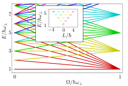
Figure 1: (Color online) Energy eigenvalues of a two dimensional harmonic oscillator as a function of angular velocity $\Omega$. For clarity only seven values of $m$ are shown, so that the infinite degeneracies at $\Omega=\omega_{\perp}$ appear to be only seven-fold. The inset shows the energy states at $\Omega=0$ as a function of their angular momentum $L$. (Colors: each Landau level is colored with a distinct hue.)

The many-body Hamiltonian, including a contact interaction $g$, is

$$H=\sum_{i=1}^{N}(h_{i}-\Omega L_{zi})+g\sum_{i>j}\delta({\bf r}_{i}-{\bf r}_{j})$$ (96)

As $\Omega\to\omega_{\perp}$, mixing is strongest among the states in the same Landau level. To simplify matters, we consider only extremely weak interactions, $gn<<2\hbar\Omega$. This limit is naturally reached when $\Omega$ is close to $\omega_{\perp}$, where the centrifugal potential largely cancels the trapping potential and the cloud becomes large and dilute. For such weak interactions, only the lowest Landau level is populated. The eigenfunctions $u_{n=0,m}({\bf r})$ in the lowest Landau level,

$$u_{m}({\bf r})=\frac{(z/d)^{m}}{\sqrt{\pi d^{2}m!}}{e^{-|z|^{2}/2d^{2}}}\equiv\langle{\bf r}|m\rangle,\,\,\,\,\,\,\,z\equiv x+iy,$$ (97)

are angular momentum eigenstates with $L=m$, and a spatial peak at $\sqrt{\langle m|r^{2}|m\rangle}=d\sqrt{2m+1}$.

The many-body wavefunction for a systems of $N$ bosons is then

$$\Psi({\bf r}_{1},...,{\bf r}_{N})=\sum_{[m]}C_{[m]}u_{m_{1}}({\bf r}_{1})...u_{m_{N}}({\bf r}_{N}),$$ (98)

where $\{m\}$ denotes the set of non-negative integers $(m_{1},m_{2},\dots m_{N})$. Since, apart from the Gaussian factor, the single particle wavefunctions are of the form $u_{m}\propto z^{m}$, the many-body wave function is

$$\Psi({\bf r}_{1},...,{\bf r}_{N})=f(z_{1},...,z_{N})e^{-\sum_{i=1}^{N}|z_{i}|^{2}/2d^{2}}$$ (99)

where $f$ is an analytic function which is symmetric in $z_{i}$. In particular, a Bose-condensed state corresponds to

$$\Psi_{w}({\bf r}_{1},...,{\bf r}_{N})=\prod_{i=1}^{N}w({\bf r}_{i}),\,\,\,\,\,\,\,\,w({\bf r})=\sum_{m}\alpha_{m}u_{m}({\bf r}).$$ (100)

If $\Psi$ is also an eigenstate of the total angular momentum $L_{z}=L$, then $f$ in Eq. (99) must be a homogeneous symmetric polynominal of $\{z_{i}\}$ of degree $L$. Moreover, the single particle density matrix in the angular momentum basis must be diagonal, i.e.,

$$\langle a^{\dagger}_{m}a_{n}\rangle=\delta_{mn}\langle a^{\dagger}_{m}a_{m}\rangle.$$ (101)

Thus a Bose condensed state (Eq. (100)) that is also an angular momentum eigenstate must be fully condensed into the single particles state $u_{m}$, i.e., $w({\bf r})=u_{m}({\bf r})$. The total angular momentum must then be $L=mN\hbar$. Such a coherent state, however, offers no flexibility to redistribute particles to lower the energy, and is therefore unlikely to be the ground state at fixed angular momentum or fixed rotational frequency $\Omega$, except for certain special cases in which parameters of the system are carefully tuned. A general Bose condensed state, Eq. (100), would be one where $w({\bf r})$ contains more than a single angular momentum state, $u_{m}$. Such states break rotational symmetry and are not angular momentum eigenstates. Furthermore, due to rotational symmetry, any rotation of $w$ ($w(r,\phi)\rightarrow w(r,\phi+\theta)$) will have the same energy and angular momentum, $L=\langle\Psi_{w}|L_{z}|\Psi_{w}\rangle$. One can therefore form an angular momentum eigenstate with angular momentum $L$ by forming the average

$$\Phi_{L}({\bf r}_{1},..{\bf r}_{N})=\int{\rm d}\theta e^{iL\theta}\Psi(\{r_{i},\phi_{i}+\theta\}).$$ (102)

Such averaging always lowers the energy of the system, and generically results in a fragmented state. Specific examples follow. Note that with small modification these arguments also apply in the general case when interactions are not weak.

III.3.2 Ground state of the rotating Bose gas with attractive interactions:

For the rotating Bose gas with attractive interaction, Wilkin, Gunn, and Smith Wilkin1998a pointed out the ground state with non-zero angular momentum is one with all angular momentum carried by the center of mass, and has the form

$$\Psi({\bf r}_{1},..{\bf r}_{N})=K(Z/d)^{L}e^{-\sum_{i=1}^{N}|z_{i}|^{2}/2d^{2}},$$ (103)

where $Z$ is the center of mass and $K$ is a normalization constant,

$$Z=\frac{1}{N}\sum_{i=1}^{N}z_{i},\,\,\,\,\,\,\,\,K=\frac{1}{\sqrt{L!(\pi d^{2})^{N}}}.$$ (104)

It is straightforward to show that the single particle density matrix of this state is

$$\langle a^{\dagger}_{m}a_{n}\rangle=\delta_{mn}N\left(\frac{L!(N-1)^{L-m}}{m!(L-m)!N^{L}}\right).$$ (105)

The ground state is fragmented because Eq. (105) has a distribution of large eigenvalues. Later, Pethick and Pitaevskii pp pointed out that this state is of the form

$$\Psi({\bf r}_{1},..{\bf r}_{N})=\Psi_{\rm CM}({\bf R})\phi_{rel}(\{\vec{\rho}_{i}\}),$$ (106)

where $\Psi_{\rm CM}({\bf R})=(Z/d)^{L}e^{-|Z|^{2}/2d^{2}}$ is the wavefunction of the center of mass ${\bf R}=\sum_{i=1}^{N}{\bf r}_{i}/N$, and $\phi_{rel}(\{\vec{\rho}_{i}\})=Ke^{-\sum_{i=1}^{N}|\vec{\rho}_{i}|^{2}/2d^{2}}$ is a product of single particle states, where the particle coordinates are $\{\vec{\rho}_{i}={\bf r}_{i}-{\bf R}\}$. Given this structure, it is natural to refer to this state as being singly condensed in the center of mass frame. Here, we show that this exact ground state can also be written as a symmetry average of broken symmetry states of the form Eq. (102), as in many of the previous examples.

Attractive interactions favor particles clumping together. In homogeneous systems, such clumping leads to collapse. In the fast rotating limit, however, the analyticity of the wavefunction in the lowest Landau level and the Gaussian factor impose strong constraints on the degree of localization possible. The most localized state is $u_{0}({\bf r})$, a Gaussian of a width given by the trap length $d$. A similar localized wave-packet at location $a\equiv a_{x}+ia_{y}$ is

$$\phi_{a}({\bf r}) = e^{(2a^{\ast}z-|z|^{2}-|a|^{2})/2d^{2}}/\sqrt{\pi}\,d,$$ (107)

$$= e^{-|z-a|^{2}/2d^{2}}e^{(a^{\ast}z-az^{\ast})/2d^{2}}/\sqrt{\pi}d,$$ (108)

which gives

$$|\phi_{a}({\bf r})|^{2}=e^{-|z-a|^{2}/2d^{2}}/\pi d^{2}.$$ (109)

A many-body coherent state formed from these single particle states is

$$\Psi({\bf r}_{1},...{\bf r}_{N})=\prod_{i=1}^{N}\phi_{a}({\bf r}_{i}).$$ (110)

This state carries angular momentum $\hbar L$ $=\langle\Psi|L_{z}|\Psi\rangle$ $=\langle\Psi|\int{\rm d}{\bf r}\psi^{\dagger}({\bf r}){\bf r}\times(\hbar\nabla/i)\psi({\bf r})|\Psi\rangle$, with

$$L=N\int{\rm d}{\bf r}|\phi_{a}({\bf r})|^{2}\left([r/d]^{2}-1\right)=N|a/d|^{2}.$$ (111)

The single particle density matrix is

$$\langle\psi^{\dagger}({\bf r^{\prime}})\psi({\bf r})\rangle=N\phi^{\ast}_{a}({\bf r^{\prime}})\phi_{a}({\bf r}),$$ (112)

in which

$$\langle a^{\dagger}_{m}a_{n}\rangle = \pi d^{2}Nu^{\ast}_{m}({\bf a})u_{n}({\bf a})$$ (113)

$$= N\left(\frac{L}{N}\right)^{m}\frac{e^{-L/N}}{m!}.$$

From this degenerate set of coherent states we construct an eigenstate of angular momentum by taking the superposition

$$\frac{1}{d^{L+2}N^{L}\sqrt{L!}}\int\frac{{\rm d}^{2}a}{2\pi}e^{-|a|^{2}/2d^{2}}a^{L}|a\rangle$$

$$=\frac{Z^{L}e^{-\sum_{i=1}^{N}|z_{i}|^{2}/2d^{2}}}{\sqrt{L!(\pi d^{2})^{N}}},$$ (114)

where $Z=\frac{1}{N}\sum_{i=1}^{N}z_{i}/d$ .

III.3.3 Fragmentation in a rotating Bose gas with repulsive interactions:

Similar fragmentation is found in the repulsive case, which for $L\ll N\hbar$ is described by a vortex lattice. A general mean field state is of the form Eq. (100), with $w({\bf r})=f(z)e^{-|z|^{2}/2d^{2}}$,

$$f(z)=\prod_{a}(z-a),$$ (115)

where the zeroes $a$ are the locations of the vortices hollvort . The angular momentum carried by this state can be obtained by noting that within the lowest Landau level,

$$\langle L_{z}\rangle=\hbar\langle\left((r/d)^{2}-1\right)\rangle,$$ (116)

which increases as the density of vortices increases. Following the arguments which we used for the attractive case, we are once again lead to a fragmented condensate (see liu for numerical studies).

The rotating Bose gas with repulsive interactions is, however, much richer than that with attractive interactions, since the mean-field picture breaks down in a fundamental way at large values of angular momentum. One sees this breakdown by first noting that with increase of the angular momentum, the vortex density increases and the particle density decreases hollvort ; baymllvort ; coresize . Eventually, the density of vortices is comparable to the density of particles and one can significantly improve the energy of the system by correlating the positions of the vortices with the positions of the particles. These correlations cannot be captured by any simple manipulation of the mean-field states; the general description of the system with large angular momentum is quite complicated hall ; wg .

Despite this complexity, there is a limit in which we can find the exact ground state. Imagine that the system is rotating with $\Omega$ sufficiently close to $\omega_{\perp}$ that the energy spacing within the lowest Landau level may be treated as a perturbation. One would find the ground state by first minimizing the interaction energy in the lowest Landau level, and then perturbatively including the level spacing. For short ranged interactions the energy is minimized by any state for which the wavefunction vanishes whenever two particles come together. Degenerate perturbation theory then says that the lowest energy state of all these wavefunctions is the one with lowest angular momentum. In the lowest Landau level, the lowest angular momentum bosonic wavefunction which vanishes when two particles touch is the $\nu=1/2$ Laughlin state,

$$\Psi([{\bf r}])=\prod_{i>j}(z_{i}-z_{j})^{2}e^{-|z_{i}|^{2}/2d^{2}}.$$ (117)

For an infinite system, one readily sees that

$$\langle a^{\dagger}_{m}a_{n}\rangle=(1/2)\delta_{mn}$$ (118)

for all $m$. Not only are there no eigenvalues of order $N$, but they are all less than unity. All traces of the conventional Bose condensation are obliterated.

IV Discussion

IV.1 Salient features

The examples shown in Sec. III share a number of common features. Many of the fragmentation processes we have discussed, such as those in Eqs. (60), (84), and (114), can be described by a family of quantum states that are weighted averages of broken symmetry states over the space of broken symmetry, typically of the form

$$|\Psi(\lambda)\rangle=\int{\rm d}\chi W(\chi,\lambda)|\chi\rangle_{c}\,\,\,,$$ (119)

where $|\chi\rangle_{c}$ is a coherent state with broken symmetry parameter $\chi$ (e.g., a spin direction), $W$ is a distribution function in the space of broken symmetry, and $\lambda$ is the parameter that controls the fragmentation of the system. If, as $\lambda$ changes, say, from $0$ to 1, $W$ changes from a distribution sharply peaked at $\chi_{0}$ to a completely uniform distribution, Eq. (119) will evolve from the coherent state $\chi_{0}$ to a fragmented state. Such changes in the distribution function reflect a growing fluctuation about the initial coherent state $\chi_{0}$ singled out by a tiny symmetry-breaking field in the coherent regime.

For example, in the case of repulsive Bose gas in a double well, $\chi$ is the relative phase between the condensates in the two wells and $\chi_{0}=0$. In the spin-1 Bose gas, $\chi$ is the vector $\hat{\bf n}$ and $\chi_{0}$ is a direction normal to an infinitesimal external magnetic field. In the rotating attractive Bose gas, $\chi$ is the location in space of the coherent state, and $\chi_{0}$ is the equilibrium location determined by, e.g., a weak potential that breaks rotational symmetry. Exactly how the fluctuations about $\chi_{0}$ grow depends on the specific dynamics of the system. Large fluctuations about $\chi_{0}$ directly reflect the competition different degenerate states for Bose condensation, the ultimate cause of fragmented structure, as discussed in the Introduction.

Another important feature of states of the type (119) is that, as a consequence of bosonic enhancement, the range of the control parameter $\lambda$ over which the system switches from a coherent to a fragmented state shrinks with particle number $N$. For a repulsive Bose gas in a double well, as discussed in Sec. III.A.2, the transition from a fragmented to a coherent takes place around $t/U>1/N$ HoCio . A similar situation occurs in the spin-1 Bose gas, where the singlet (fragmented) state gives way to a coherent state for field gradient $G>1/N$ Ho1999a . Since the window for fragmentation vanishes as $N$ increases, fragmented condensates will not be realized in condensed matter systems, with $N\sim 10^{23}$ particles. On the other hand, in mesocopic systems like quantum gases with typically $N\sim 10^{6}$ particles, fragmented states can exist in parameter ranges accessible to experiment.

Although our discussions have mainly focussed on the class of states Eq. (119), other fragmentation processes do not lead to states that are most naturally expressed in this manner, e.g., the Schrödinger-cat family in Eq. (61). One can have distinct fragmented states, such as the Fock state and the Schrödinger-cat state, with entirely different properties but identical single particle density matrices. Such different states are therefore indistinguishable within the Penrose-Onsager scheme. To tell them apart, it is necessary to examine second order correlation functions such as number fluctuations. Even higher order correlation functions are needed to distinguish the fragmented states of more complicated systems, such as those of $F=2$ Bose gases of ⁸⁷Rb, and the recently realized spin-3 Bose gas of ⁵²Cr pfau . In general, one can expect a large variety of fragmented states, differing from each other by high order correlation functions.

The relative number fluctuations of a fragmented state (such as those in the pseudo-spin 1/2 and spin-1 Bose gases discussed in Sec. III) are a measure of the stability of the state. Huge fluctuations, such as in the Schrödinger-cat state and the singlet state of the spin-1 Bose gas indicate that the system is easily damaged by external perturbations. Consider, for example, a perturbation of the form $H^{\prime}=\eta c^{\dagger}a_{1}+{\rm h.c.}$, where $a_{1}$ is a boson in one of the wells in the double well example, or a boson in the $S_{z}=1$ spin state of a spin-1 Bose gas, $c^{\dagger}$ adds a particle in a different atomic state of the same boson (e.g., a plane wave state in the background gas), and $\eta$ is a very small parameter. The perturbation $H^{\prime}$ acting on the Fock state $a^{\dagger N/2}_{1}a^{\dagger N/2}_{2}|0\rangle$ simply changes it to another Fock state, $c^{\dagger}a^{\dagger N/2-1}_{1}a^{\dagger N/2}_{2}|0\rangle$, which also has zero number fluctuations, $\langle N_{1}^{2}-\langle N_{1}\rangle^{2}\rangle=0$. In contrast, $H^{\prime}$ acting on the Schrödinger-cat state $(a^{\dagger N}_{1}+a^{\dagger N}_{2})|0\rangle$ collapses it into the state $c^{\dagger}a^{\dagger N-1}_{1}|0\rangle$, immediately reducing the enormous number fluctuations of the Schrödinger-cat state to zero. More generally, if the cat state $|\Psi_{\rm Cat}\rangle=|\Psi_{1}\rangle+|\Psi_{2}\rangle$ is a sum of two Gaussians in number space, as shown in Eq. (61), with one Gaussian ($|\Psi_{1}\rangle$) peaked at $|N_{+},N_{-}\rangle$ and the other ($|\Psi_{2}\rangle$) peaked at $|N_{-},N_{+}\rangle$, where $N_{+}+N_{-}=N$, and $N_{+}>>N_{-}$, the action of $H^{\prime}$ on $|\Psi_{\rm Cat}\rangle$ considerably enhances $|\Psi_{1}\rangle$ and suppresses $|\Psi_{2}\rangle$.

The large effect of the small perturbation $H^{\prime}$ is due to bosonic enhancement, which gives $H^{\prime}|N_{+},N_{-}\rangle=\sqrt{N_{+}}\,\,c^{\dagger}|N_{+}-1,N_{-}\rangle$ and $H^{\prime}|N_{-},N_{+}\rangle=\sqrt{N_{-}}\,\,c^{\dagger}|N_{-}-1,N_{+}\rangle$. Since $N_{+}>>N_{-}$, the norm of $H^{\prime}|N_{-},N_{+}\rangle$ is considerably smaller than that of $H^{\prime}|N_{+},N_{-}\rangle$. As a result, $H^{\prime}|\Psi_{\rm Cat}\rangle\approx H^{\prime}|\Psi_{1}\rangle\approx\sqrt{N_{+}}c^{\dagger}|N_{+}-1,N_{-}\rangle$, which is no longer a Schrödinger-cat state. In a spin-1 Bose gas, a similar action changes the singlet state $(2a^{\dagger}_{1}a^{\dagger}_{-1}-a^{\dagger 2}_{0})^{N/2}|0\rangle$ to one with much smaller relative number fluctuations.

Since Schrödinger cat-like states can collapse into Fock states with the slightest perturbation, and Fock states can easily be reassembled into a single condensate by any small amount of tunneling between different fragmented pieces, why should one bother with fragmented states? Is fragmentation relevant? The point, as mentioned before, is that even though fragmented states cannot be realized in macroscopic systems, the situation is different for mesoscopic systems like trapped quantum gases. The huge reduction in particle number considerably relaxes the constraint of formation of Fock states and Schrödinger cat-like states, and fragmented ground states become realizable. The phenomena of fragmentation becomes even richer if it takes place in both real and spin space, such as with high spin bosons in an optical lattices close to the Mott limit. The combined effect of spin degeneracy and spatial degeneracy (due to different isolated wells) produces a great variety of quantum phases as the spin of boson increases. In addition, the singlet ground state of a spin-1 Bose gas can also be viewed as a “resource” for singlets and may therefore be useful in developing quantum teleportation protocols in optical lattices with spin-1 bosons. Our understanding of the properties of fragmented states, and in particular their dynamics, is at such an early stage that it leaves open considerable room for inventive ideas, which is where the excitement lies.

We stress that we have described only the simplest types of fragmented states. Many other kinds which do not fall into the category we considered. The $\nu=1/2$ Laughlin state discussed in Sec. III.C.3 is an example at the other extreme. There are no large eigenvalues singled out in the density matrix. Instead, all the eigenvalues are identical and of order unity. In addition to level degeneracy, temperature effects can cause condensates to fragment, a subject to which we turn in the next section.

IV.2 Role of temperature

Up to this point, the examples of fragmentation given in this paper have focussed on the case where interaction-driven quantum fluctuations break up the condensate. It is intuitively clear that thermal fluctuations can play a similar role. A trivial example is given by a non-interacting Josephson junction, governed by the Hamiltonian

$$H=-t(a^{\dagger}b+b^{\dagger}a).$$ (120)

This Hamiltonian is diagonal in the basis of symmetric and asymmetric states, for which the creation operators are $(a^{\dagger}+b^{\dagger})/\sqrt{2}$, and $(a^{\dagger}-b^{\dagger})/\sqrt{2}$, so the single particle density matrix is diagonal in this basis. At zero temperature only the symmetric state is occupied – a single condensate. At very large temperature each of these states is equally occupied so the system is fragmented. For intermediate temperatures, the occupation of each of these states is

$$n_{\stackrel{{\scriptstyle\scriptscriptstyle\rm s}}{{\scriptscriptstyle\rm a}}} = \frac{\sum_{m=-N/2}^{N/2}(N/2\pm m)e^{2t\beta m}}{\sum_{m=-N/2}^{N/2}e^{2t\beta m}}$$

$$= \frac{N}{2}\mp\left(\frac{N+1}{2}\coth(\beta t(N+1))-\frac{1}{2}\coth(\beta t)\right).$$

The upper signs denote the symmetric state (s) and the lower the antisymmetric state (a). The crossover between the singly condensed state at $T=0$ and the fragmented state at $T\gg t$ is smooth. Extensions of this argument are relevant for spinor condensates in which one can, in principle, have a hierarchy of transition temperatures, where the $k=0$ mode becomes macroscopically occupied below some temperature $T_{c}$, but order in the spin-channel does not occur until a lower temperature isoshima2000a .

A vortex lattice provides a qualitatively different example of how finite temperature fragments a condensate. Imagine a bucket of ⁴He rotating at frequency $\Omega$. The ground state of the system contains a triangular array of vortices with $n_{\rm v}$ vortices per unit area. At finite temperature the vortex lattice is thermally excited, giving rise to a decay in the phase correlations across the sample. If we let $\psi(r)$ be the superfluid order parameter coarse-grained on a scale large compared to the vortex spacing, then according to baymvortex ; baymllvort , the correlation function $\langle\psi^{*}(r^{\prime})\psi(r^{\prime})\rangle$ decays as $|r-r^{\prime}|^{-\eta}$, for large separations. The exponent $\eta=1/(3\pi^{2}\rho r_{\rm v}\Lambda^{2})$ is proportional to the ratio of the distance between particles to the distance between vortices. Here the particle number density is $\rho$, the thermal wavelength is $\Lambda=\sqrt{2\pi/mk_{b}T}$ and the distance between vortices is $r_{\rm v}$. This algebraic decay of correlations in real space corresponds to an algebraic decay in momentum space. For $\eta<3$, the occupation of the $k=0$ mode scale as $N_{0}\sim L^{3-\eta}$, and as as $k\to 0$ the occupations of the $k\neq 0$ modes scale as $N_{k}\sim k^{\eta-3}$. Thus the number of macroscopically occupied modes scales as $L^{\eta}$, and for carefully chosen $L$ and $\eta$ a fragmented state can result.

For a typical helium experiment $\eta<10^{-8}$, and the depletion caused by this effect is negligible. Experiments on alkali gases, e.g., mitvort ; jilavort , create vortex lattices with $r_{\rm v}\sim 5\mu$m and a particle density $\rho\sim 10^{14}$ cm^-3, for which $\eta\sim 10^{-3}$, also a minor correction. Experiments with smaller vortex lattices in Paris Madison2000a have a similar vortex spacing $r_{\rm v}\sim 2\mu$m, and density $\rho\sim 10^{14}$ cm^-3, yielding a comparable value for $\eta$. Although vortex lattices in current experiments are not thermally fragmented, there does not appear to be any fundamental impediment to making $\eta$ larger.

IV.3 Other recent work

Not surprisingly, given the fascinating nature of fragmented states, several recent papers (all cited in the relevant sections of this paper) have been investigating models similar to those discussed here. As a guide to the reader, we briefly summarize these works, presenting them in roughly the same order as they appear in the main text.

The two-state system was explored by Nozières Nozieres1995a , who pointed out the existence of fragmentation in that system. The generic stability of a two-state fragmented condensate was considered by Rokhsar Rokhsar1998a . One realization of this model would be to place atoms in bonafide double-well potentials. Due to mode mixing such a system is not identical to a simple two-mode model, and several authors have explored more realistic models. Spekkens and Sipe spekkens used a variational approach to compare fragmented and singly condensed states in such potentials. More recently, Streltsov and Cederbaum streltsov , along with Moiseyev cedermos produced similar results through a multi-mode mean-field theory. The evolution of the ground state from a Fock state to a coherent state and from a coherent state to a Schrödinger-cat state was studied by Ho and Ciobanu HoCio . Experiments have recently produced a condensate confined in a double-well trap dwexp .

The fragmented nature of the ground state of the spin-1 Bose gas was first noted by Nozières and Saint James nsj . Later studies by Law, Pu, and Bigelow Law1998c investigated the ground state properties and the spin dynamics in terms of the basis used in Eq. (88). Ho and Yip Ho1999a showed that the fragmented singlet state has huge fluctuations; they also showed the relation between this fragmentation and spontaneous symmetry breaking. They explicitly showed how magnetic fields and field gradients drive the system into a singly condensed state. Similar considerations were addressed by Koashi and Ueda Koashi . Javanainen discussed Issues involving the measurement of the fragmented spin-1 ground state jav .

The rotating attractive gas was first studied by Wilkin et al. Wilkin1998a , who noted that the ground state was fragmented. The connection between this fragmentation and symmetry breaking was first discussed by Pethick and Pitaevskii pp .

There have been extensive studies of the properties of the rotating repulsive gas in the lowest Landau level – many of which have focussed on the structure of the order in the single particle density matrix. These works have mainly used a combination of exact diagonalization and variational techniques. A particularly relevant paper is the exact diagonalization study of Liu et al. liu , which focusses on the symmetry-breaking nature of the vortex states. A related paper by Jackson et al. jackson compares mean-field and exact wavefunctions at various values of the angular momentum. The Goldstone mode associated with vortex nucleation was discussed by Ueda and Nakajima UedaNakajima .

Fragmentation occurs in “clumped” bosonic systems with attractive interactions. Ueda and Leggett used a two-mode approximation uedaleggett to study fragmentation and soliton formation in a one dimensional attractive Bose gas. A quite thorough comparison of mean-field theory and exact diagonalzation is found in the articles by Kanamoto et al. kanamoto , as well as the closely related work of Kavoulakis kav2003 . Montina and Arecchi montina use a Monte-Carlo scheme to investigate the degree of fragmentation of this system. In three dimensions, Elgaroy and Pethick peth showed that a harmonically trapped gas of atoms with attractive interactions does not form a stable fragmented state.

Other systems with symmetry breaking and fragmentation include phase separated two-component gases esry1999 , and rotating gases during a phase-slip event muellerswallowtails . Boson ground states where the condensate is broken into a macroscopic number of pieces include the Mott insulator mott , fractional quantum Hall states hall ; wg , and the low dimensional Bose gas lowd ; twoquasi . Aspects of the dynamics of regaining phase coherence among condensates are discussed by Yi and Duan dynamics , a paper closely related to discussion of how the measurement process is influenced by fragmentation Javmeasure ; castindalibard .

Finally we mention the lecture notes produced by Castin and Herzog for the 2000 Cargèse Summer School castin , which lucidly introduces fragmentation and analyzes the case of spin-1 bosons and of the one-dimensional attractive gas. They included an extended discussion of the role of symmetry breaking.

V Summary

Bose condensation is remarkably robust. It is therefore exciting to search for zero-temperature bosonic states which are not condensed and to understand the process that breaks up the condensate. Fragmentation, where the condensate breaks up into a few pieces, is the first step in this journey, which eventually ends at strongly-correlated states possessing no trace of condensation.

We have described some of the canonical models which have fragmented ground states, and extracted their properties. We see that there is a rich variety of fragmented ground states. Often fragmentation is associated with restoring a broken symmetry. Sometimes it is accompanied by order in higher-order correlation functions. The one unifying feature appears to be a combination of near-degeneracies and interactions. The higher the degree of degeneracy, the more fragmented the condensate may become.

VI Acknowledgements

Parts of this research were performed at the Aspen Center for Physics and the Kavli Institute for Theoretical Physics in Santa-Barbara. The authors acknowledge the following support: EJM – NSF Grant PHY-0456261 and the Sloan foundation; TLH – NSF Grant DMR-0426149 and NASA GRANT-NAG8-1765; MU – Grants-in-Aids for Scientfic Research (Grant No. 17071005) and a CREST program of the JST; and GB – NSF Grant PHY03-55014 and PHY05-00914.

References

- (1) K. Huang, Statistical Mechanics (2nd Ed.), (Wiley, 1987).
- (2) A. Einstein, Ber. Berl. Akad. 261 (1924); 3 (1925).
- (3) F. London, Phys. Rev. 54, 947 (1938).
- (4) N. N. Bogoliubov, J. Phys. (USSR) 11, 23 (1947); reprinted in D. Pines, The Many-Body Problem, (W. A. Benjamin, New York, 1961).
- (5) O. Penrose and L. Onsager, Phys. Rev. 104, 576 (1956).
- (6) C. J. Pethick and H. Smith, Bose-Einstein Condensation in Dilute Gases, (Cambridge Univ. Press, Cambridge, 2002).
- (7) P. Nozières and D. Saint James, J. Physique 43, 1133 (1982).
- (8) P. Nozières, in Bose-Einstein Condensation, edited by A. Griffin, D. W. Snoke, and S. Stringari (Cambridge University Press, Cambridge, 1995).
- (9) N. Wilkin, J. Gunn, and R. Smith, Phys. Rev. Lett. 80, 2265 (1998).
- (10) M. Girardeau, Phys. Fluids 5, 1468 (1962).
- (11) M. Koashi and M. Ueda, Phys. Rev. Lett. 84, 1066 (2000).
- (12) T.-L. Ho and S. K. Yip, Phys. Rev. Lett. 84, 4031 (2000).
- (13) Y. Castin and C. Herzog, “Bose-Einstein condensates in symmetry breaking states”, Comptes Rendus de l’Academie des Sciences de Paris, tome 2, serie IV, 419 (2001). Also available as cond-mat/0012040.
- (14) O. Elgaroy and C. J. Pethick, Phys. Rev. A 59, 1711 (1999).
- (15) D. S. Rokhsar, Phase coherence and “fragmented” Bose condensates (1998), cond-mat/9812260.
- (16) R. W. Spekkens and J. E. Sipe, Phys. Rev. A 59, 3868 (1999).
- (17) J. Javanainen, J. Phys. B 33, 5493 (2000).
- (18) J. Dukelsky and P. Schuck, Phys. Rev. Lett. 86, 4207 (2001).
- (19) C.J. Myatt, E.A. Burt, R.W. Ghrist, E.A. Cornell and C.E. Wieman, Phys. Rev. Lett. 78, 586 (1997); M.R. Matthews, D.S. Hall, D.S. Jin, J.R. Ensher, C. Wieman, E.A. Cornell, F. Dalfovo, C. Minniti, and S. Stringari, Phys. Rev. Lett. 81, 243 (1998); D. S. Hall, M.R. Matthews, J.R. Ensher, C.E. Wieman, and E.A. Cornell, Phys. Rev. Lett. 81, 1539 (1998); D.S. Hall, M.R. Matthews, C.E. Wieman, and E.A. Cornell, Phys. Rev. Lett. 81, 1543 (1998); M.R. Matthews, B.P. Anderson, P.C. Haljan, D.S. Hall, M.J. Holland, J.E Williams, C.E. Wieman, E.A. Cornell, Phys. Rev. Lett. 83, 3358 (1999).
- (20) A. Görlitz, T.L. Gustavson, A.E. Leanhardt, R. Löw, A.P. Chikkatur, S. Gupta, S. Inouye, D.E. Pritchard, and W. Ketterle, Phys. Rev. Lett. 90, 090401 (2003); D.M. Stamper-Kurn, H.-J. Miesner, A.P. Chikkatur, S. Inouye, J. Stenger, and W. Ketterle: Phys. Rev. Lett. 83, 661 (1999). H.-J. Miesner, D.M. Stamper-Kurn, J. Stenger, S. Inouye, A.P. Chikkatur, and W. Ketterle: Phys. Rev. Lett. 82, 2228 (1999). J. Stenger, S. Inouye, D.M. Stamper-Kurn, H.-J. Miesner, A.P. Chikkatur, and W. Ketterle: Nature 396, 345 (1998). D.M. Stamper-Kurn, M.R. Andrews, A.P. Chikkatur, S. Inouye, H.-J. Miesner, J. Stenger, and W. Ketterle: Phys. Rev. Lett. 80, 2027 (1998); J. M. Higbie, L. E. Sadler, S. Inouye, A. P. Chikkatur, S.R. Leslie, K.L. Moore, V. Savalli, and D.M. Stamper-Kurn. Phys. Rev. Lett. 95, 050401 (2005); M.-S. Chang, C.D. Hamley, M.D. Barrett, J.A. Sauer, K.M. Fortier, W. Zhang, L. You, and M.S. Chapman, Phys. Rev. Lett. 92, 140403 (2004); H. Schmaljohann, M. Erhard, J. Kronjäger, M. Kottke, S. van Staa, L. Cacciapuoti, J.J. Arlt, K. Bongs, and K. Sengstock, Phys. Rev. Lett. 92, 040402 (2004); and T. Kuwamoto, K. Araki, T. Eno, and T. Hirano, Phys. Rev. A 69, 063604 (2004).
- (21) H. Moritz, T. Stöferle, M. Köhl, and T. Esslinger, Phys. Rev. Lett. 91, 250402 (2003); T. Stöferle, H. Moritz, C. Schori, M. Köhl, and T. Esslinger, Phys. Rev. Lett. 92, 130403 (2004).
- (22) M. Greiner, O. Mandel, T. Esslinger, T. W. Hansch, and I. Bloch, Nature, 415, 39 (2002); and M. P. A. Fisher, P. B. Weichmann, G. Grinstein, and D. S. Fisher, Phys. Rev. B 40, 546 (1989).
- (23) N.R. Cooper and N.K. Wilkin, Phys. Rev. B 60, R16279 (1999); S. Viefers, T.H. Hansson, and S.M. Reimann, Phys. Rev. A 62, 053604 (2000); N.R. Cooper, N.K. Wilkin, and J.M.F. Gunn, Rev. Lett. 87, 120405 (2001); B. Paredes, P. Fedichev, J.I. Cirac, and P. Zoller, Rev. Lett. 87, 010402 (2001); J.W. Reijnders, F.J.M. van Lankvelt, K. Schoutens, and N. Read, Phys. Rev. Lett. 89, 120401 (2002); B. Paredes, P. Zoller, and J.I. Cirac, Phys. Rev. A 66, 033609 (2002); N. Regnault, and Th. Jolicoeur, Phys. Rev. Lett. 91, 030402 (2003); and T. Nakajima and M. Ueda, Phys. Rev. Lett. 91, 140401 (2003).
- (24) N.K. Wilkin and J.M.F. Gunn, Phys. Rev. Lett. 84, 6 (2000).
- (25) O. Penrose, Phil. Mag. 42, 1373 (1951).
- (26) See, e.g., J.L. DuBois and H.R. Glyde, Phys. Rev. A 68, 033602 (2003).
- (27) T. Papenbrock, Phys. Rev. A 67, 041601(R) (2003); D.M. Gangardt, and G.V. Shlyapnikov, Phys. Rev. Lett. 90, 010401 (2003); M.D. Girardeau, E.M. Wright, and J.M. Triscari, Phys. Rev. A 63, 033601 (2001); D.S. Petrov, G.V. Shlyapnikov, and J.T.M. Walraven, Phys. Rev. Lett. 85, 3745 (2000); and A. Lenard, J. Math. Phys. 7, 1268 (1966).
- (28) J. Javanainen and S. M. Yoo, Phys. Rev. Lett. 76, 161 (1996).
- (29) Y. Castin and J. Dalibard, Phys. Rev. A 50, 4330 (1997).
- (30) M. R. Andrews, C. G. Townsend, H.-J. Miesner, D. S. Durfee, D. M. Kurn, and W. Ketterle, Science 275, 637 (1997); M. R. Andrews, D. M. Kurn, H.-J. Miesner, D. S. Durfee, C. G. Townsend, S. Inouye, and W. Ketterle, Phys. Rev. Lett. 79, 553 (1997); ibid. 80, 2967 (1998).
- (31) The real puzzle is why each single shot measurement yields an interference pattern of two phase-coherent condensates with an apparent relative phase . The explanation, which is not contained in Eq.(22), lies in quantum measurement theory; the very act of measurement actually establishes a phase between the two initially incoherent condensates, a phenomenon that is a consequence of bosonic enhancement castindalibard .
- (32) M. Albiez, R. Gati, J. Fölling, S. Hunsmann, M. Cristiani, and M.K. Oberthaler, Phys. Rev. Lett. 95, 010402 (2005).
- (33) M. Ueda and A.J. Leggett, Phys. Rev. Lett. 83, 1489 (1999).
- (34) E.J. Mueller, Phys. Rev. A 66, 063603 (2002).
- (35) G. Baym, Lectures on Quantum Mechanics, W. A. Benjamin, Inc., New York, 1969.
- (36) By a suitable change of variables one can make the hopping uniform, but at the cost of making the potential more complicated. See G. Scharf, W. F. Wreszinski, and J. L. van Hemmen, J. Phys. A: Math. Gen. 20, 4309 (1987).
- (37) T.-L. Ho and C.V. Ciobanu, J. Low Temp. Phys. 125, 257 (2004).
- (38) H. Schmaljohann, M. Erhard, J. Kronjäger, M. Kottke, S. van Staa, L. Cacciapuoti, J.J. Arlt, K. Bongs, and K. Sengstock, Phys. Rev. Lett. 92, 040402 (2004).
- (39) T. Kuwamoto, K. Araki, T. Eno, and T. Hirano, Phys. Rev. A 69, 063604 (2004).
- (40) W. Zhang, D.L. Zhou, M.-S. Chang, M.S. Chapman, and L. You, Phys. Rev. A 72, 013602 (2005); and M.-S. Chang, Q. Qin, W. Zhang, L. You, M.S. Chapman, cond-mat/0509341 (2005).
- (41) H. Saito and M. Ueda, Phys. Rev. A 72, 023610 (2005).
- (42) T.L. Ho, Phys. Rev. Lett. 81, 742 (1998).
- (43) T.-L. Ho and L. Yin, Phys. Rev. Lett. 84, 2302 (2000).
- (44) M. Ueda and M. Koashi, Phys. Rev. A 65, 063602 (2002).
- (45) C.K. Law, H. Pu, and N.P. Bigelow, Phys. Rev. Lett. 81, 5257 (1998).
- (46) C.J. Pethick and L. Pitaevskii, Phys. Rev. A 62, 033609 (2000).
- (47) T.-L. Ho, Phys. Rev. Lett. 87, 060403 (2001).
- (48) X.-J. Liu, H. Hu, L. Chang, W. Zhang, S.-Q. Li, and Y.-Z, Wang, Phys. Rev. Lett. 87, 030404 (2001).
- (49) G. Baym, Phys. Rev. A 69, 043618 (2004).
- (50) G. Baym and C.J. Pethick, Phys. Rev. A 69, 043619 (2004).
- (51) A. Griesmaier, J. Werner, S. Hensler, J. Stuhler, and T. Pfau, Phys. Rev. Lett. 94, 160401 (2005); cond-mat/0503044; and A. Griesmaier, J. Stuhler, and T. Pfau, cond-mat/0508423.
- (52) T. Isoshima, T. Ohmi, and K. Machida, J. Phys. Soc. Jpn. 69, 3864 (2000).
- (53) G. Baym, Phys. Rev. B 51, 11697 (1995).
- (54) J. R. Abo-Shaeer, C. Raman, J. M. Vogels, W. Ketterle, Science, 292, 476 (2001).
- (55) V. Schweikhard, I. Coddington, P. Engels, V. P. Mogendorff, and E. A. Cornell, Phys. Rev. Lett. 92, 040404 (2004); I. Coddington, P. C. Haljan, P. Engels, V. Schweikhard, S. Tung, and E. A. Cornell, Phys. Rev. A 70, 063607 (2004); and references therein.
- (56) K.W. Madison, F. Chevy, W. Wohlleben, and J. Dalibard, Phys. Rev. Lett. 84, 806 (2000).
- (57) A.I. Streltsov and L.S. Cederbaum, Phys. Rev. A 71, 063612 (2005).
- (58) A.I. Streltsov, L.S. Cederbaum, and N. Moiseyev, Phys. Rev. A 70, 053607 (2004).
- (59) A.D. Jackson, G.M. Kavoulakis, B. Mottelson, and S.M. Reimann, Phys. Rev. Lett. 86, 945 (2001).
- (60) M. Ueda and T. Nakajima, Phys. Rev. A 73, 043603 (2006).
- (61) R. Kanamoto, H. Saito, and M. Ueda, Phys. Rev. A 67, 013608 (2003); 68, 043619 (2003); and Phys. Rev. Lett. 94, 090404 (2005).
- (62) G. M. Kavoulakis, Phys. Rev. A, 67, 011601(R) (2003); 69, 023613 (2004).
- (63) A. Montina and F. T. Arecchi, Phys. Rev. A 71, 063615 (2005).
- (64) B. D. Esry, and C. H. Greene, Phys. Rev. A, 59, 1457 (1999).
- (65) Y. Kagan, V.A. Kashurnikov, A.V. Krasavin, N.V. Prokof’ev, and B.V. Svistunov, Phys. Rev. A 61, 043608 (2000); J.M. Kosterlitz and D.J. Thouless, J. Phys. C 6 1181 (1973); D.S. Petrov, M. Holzmann, and G.V. Shlyapnikov, Phys. Rev. Lett. 84, 2551 (2000); D.S. Fisher and P. C. Hohenberg, Phys. Rev. B, 37, 4936 (1988); V. N. Popov, Functional Integrals in Quantum Field Theory and Statistical Physics, (Reidel, Dordrecht, 1983).
- (66) W. Yi and L.-M. Duan, Phys. Rev. A 71, 043607 (2005).