Theory of vortex-lattice melting in a one-dimensional optical lattice

Abstract

We investigate quantum and temperature fluctuations of a vortex lattice in a one-dimensional optical lattice. We discuss in particular the Bloch bands of the Tkachenko modes and calculate the correlation function of the vortex positions along the direction of the optical lattice. Because of the small number of particles in the pancake Bose-Einstein condensates at every site of the optical lattice, finite-size effects become very important. Moreover, the fluctuations in the vortex positions are inhomogeneous due to the inhomogeneous density. As a result, the melting of the lattice occurs from the outside inwards. However, tunneling between neighboring pancakes substantially reduces the inhomogeneity as well as the size of the fluctuations. On the other hand, nonzero temperatures increase the size of the fluctuations dramatically. We calculate the crossover temperature from quantum melting to classical melting. We also investigate melting in the presence of a quartic radial potential, where a liquid can form in the center instead of at the outer edge of the pancake Bose-Einstein condensates.

I Introduction

Since the onset of experiments on Bose-Einstein condensates, vortices have attracted a lot of attention. When the Bose-Einstein condensate is rotated faster than some critical rotation frequency $\Omega_{c}$, a vortex appears in the gas Matthews99 ; Madison00 ; Fetter01_JP . Upon increasing the rotation frequency further, the number of vortices increases Hodby01 ; Hodby02 ; Rosenbusch02 ; Leanhardt02 ; Leanhardt03 , and the vortices order themselves in a hexagonal Abrikosov lattice Abo-Shaeer01 ; Abo-Shaeer02 ; Engels02 ; Engels03 ; Coddington03 ; Schweikhard04 ; Bretin04 . If the rotation frequency is increased even further, the very rapidly rotating ultracold bosonic gases have been predicted to form highly-correlated quantum states Wilkin98 ; Cooper99 ; Wilkin00 ; Cooper01 ; Ho02 . In these states, the Bose-Einstein condensate has been completely depleted by quantum fluctuations, and quantum liquids appear with excitations that can carry fractional statistics. Some of these states have been identified with (bosonic) fractional quantum Hall states Cooper01 ; Paredes02 ; Regnault03 , such as the Laughlin state Laughlin83 , the Moore-Read state Moore91 and various Read-Rezayi states Read99 ; Rezayi05 .

In this article we study the quantum fluctuations of vortices in a one-dimensional optical lattice. Optical lattices provide a powerful tool in manipulating a Bose-Einstein condensate. By using a three-dimensional optical lattice, the Bose-Hubbard model Jaksch98 was experimentally realized and the superfluid-Mott insulator transition was observed Greiner02 . Moreover, a two-dimensional optical lattice was used to create one-dimensional Bose-gases and to study the crossover between a superfluid Bose gas and the “fermionized” Tonks gas Paredes04 ; Kinoshita04 . Theoretically, the combination of a two-dimensional optical lattice and a single vortex was predicted to give interesting effects around the superfluid-Mott insulator transition Wu04 . Optical lattices can also be used to provide a pinning potential for vortices Reijnders04 ; Reijnders05 ; Pu05 ; Bhat06 ; Burkov06 , and experiments on this topic are ongoing Cornell05 . The physics of a single vortex line in a one-dimensional optical lattice is recently extensively studied Martikainen03 ; Martikainen03B ; Martikainen04 ; Martikainen04B ; Martikainen04C ; Isoshima05 . By putting fermions in the vortex core, this system can even be used to create a superstring in the laboratory Snoek05 .

A one-dimensional optical lattice divides the Bose-Einstein condensate into a stack of two-dimensional pancake condensates that are weakly coupled by tunneling as schematically shown in Fig. 1. An important consequence of this setup is that the modes of the on-site two-dimensional vortex lattice form Bloch bands as a function of the axial momentum. In this paper we pay special attention to the Tkachenko modes Tkachenko66 , which are the lowest-lying modes of the vortex lattice. Recently, these modes have been investigated for a single two-dimensional vortex lattice both experimentally Schweikhard04 ; Coddington03 and theoretically Baym03 ; Mizushima04 ; Baksmaty04 ; Baym04 ; Kim04 ; Cozzini04 ; Sonin05 ; Sonin05B .

The number of particles in a single pancake is much smaller than in a Bose-Einstein condensate in a harmonic trap, and hence the fluctuations are much larger. Therefore, this system is a promising candidate to reach the quantum Hall regime. The requirement for that is that the ratio $\nu=N/N_{v}$ of the number of atoms $N$ and the number of vortices $N_{v}$ is smaller than a critical value $\nu_{c}$. The ratio $\nu$ plays the role of the filling factor and estimates for the critical $\nu_{c}$ are typically around $8$ Cooper01 ; Sinova02 . However, observed filling factors are up till now always greater than 100, where almost perfect hexagonal lattices form and no sign of melting can be seen Schweikhard04 . These experiments are carried out with Bose-Einstein condensates consisting of typically $10^{5}$ particles, whereas the maximum number of vortices observed is around $300$. Decreasing the number of particles results in loss of signal, whereas the number of vortices is limited by the rotation frequency that has to be smaller than the transverse trapping frequency. Adding a quartic potential, which stabilizes the condensate also for rotation frequencies higher than the transverse trap frequency, has until now not improved this situation Bretin04 , although it has opened up the possibility of forming a giant vortex in the center of the cloud Lundh02 ; Kasamatsu02 ; Kavoulakis03 . Applying a one-dimensional optical lattice produces pancake condensates each containing typically 1000 particles, such that quantum fluctuations are strongly enhanced. Experimental signal is still conserved because of the combined signal of all the pancake. Moreover, because of the small number of particles in each pancake shaped Bose-Einstein condensate, finite-size effects become very pronounced in this setup. In particular, the critical filling factor for the melting of the lattice $\nu_{c}$ changes compared to the homogeneous situation. As a further consequence, melting is not expected to occur homogeneously but starts at the outside and then gradually moves inwards as the rotation speed increases Fischer04 . Therefore, phase coexistence is expected, where a vortex crystal is surrounded by a vortex liquid.

The optical lattice gives also the exciting possibility to study the dimensional crossover between two-dimensional melting and three-dimensional melting, by varying the coupling between the pancakes. This system also exhibits an intruiging similarity to the layered structure of the high-$T_{c}$ superconductors Rozhkov96 ; Col05 . Recently, the density profiles for quantum Hall liquids in this geometry have been calculated Cooper05 . Also the static properties of the lattice in a double and multilayer geometry have been investigated Zhai04 ; Zhang05 . Finally, classical melting between shells of vortices in a single two-dimensional Bose-Einstein condensate has also been studied recently Pogosov06 .

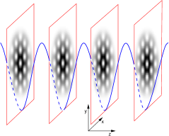
Figure 1: (Color online) Setup in which the melting of the vortex lattice is studied. An optical lattice along the $z$ direction divides the condensate into pancake condensate which are coupled by tunneling processes.

In this article we study this interesting physics by expanding on our previous work Snoek06 . The paper is organized as follows. In Sec. II we present the theoretical foundations of our work and derive the effective lagrangian for the vortex fluctuations. In Sec. III we discuss the excitation spectrum and we pay in particular attention to the Bloch bands of the Tkachenko modes. In Sec. IV we present result on the quantum melting, and in Sec. V we take into account the effects of a nonzero temperature. We calculate the crossover temperature from quantum melting to classical melting. In Sec. VI we present results on the addition of a quartic potential. We end up with conclusions in Sec. VII.

II Effective Lagrangian

In this section we derive the effective lagrangian for the vortex fluctuations. Using the ansatz that the condensates wavefunctions are part of the lowest Landau level, we find the classical groundstates and expand the action up to second order in the fluctuations.

II.1 Tight-binding approximation

We closely follow the approach in Ref. Martikainen04 for a single vortex, extending it to the case of a vortex lattice. Our starting point is a cigar-shaped Bose-Einstein condensate trapped by the potential

$$V({\bf r})=\frac{m}{2}(\omega_{\perp}^{2}r^{2}+\omega_{z}^{2}z^{2}),$$ (1)

where $m$ is the atomic mass and $\omega_{r}$ and $\omega_{z}$ are the radial and axial trapping frequencies, respectively. Since we assume a cigar-shaped trap, we have that $\omega_{z}\ll\omega_{\perp}$ and we neglect the axial trapping in the rest of this work. Experimentally this can also be realized by using end-cap lasers, which results in a box-like trapping potential in axial direction Strecker02 . In addition, the Bose-Einstein condensate experiences a one-dimensional optical lattice

$$V_{z}({\bf r})=V_{z}\sin^{2}\left(\frac{2\pi z}{\lambda}\right),$$ (2)

where $V_{z}$ is the lattice depth and $\lambda$ is the wavelength of the laser light. The lattice potential splits the condensate into $N_{s}$ two-dimensional condensates with a pancake shape. Each of the pancake Bose-Einstein condensates contains on average $N$ atoms, so the total number of atoms is $N_{s}N$. We consider a deep optical lattice, such that its depth is larger than the chemical potential of the two-dimensional condensate, but still we assume that there is full coherence across the condensate array. This means in particular that the lattice potential should not be so deep as to induce a superfluid-Mott insulator transition. Typically the required lattice depth to reach the superfluid-Mott insulator transition in a three-dimensional lattice with one particle per lattice site is of the order of $10E_{z}$, where $E_{z}$ is the recoil energy of an atom after absorbing a photon from the laser beam and given by

$$E_{z}=\frac{(2\pi\hbar/\lambda)^{2}}{2m}.$$ (3)

In a one-dimensional lattice the number of atoms in each lattice site is typically much larger than in a three-dimensional lattice and the transition into the insulating state requires a much deeper lattice Oosten03 . The superfluid-Mott insulator transition in a one-dimensional optical lattice has recently been observed Stoferle04 , but also in that case the number of particles per lattice site is of the order of one.

The action describing the system in the rotating frame is given by $S=\int dt\int d^{3}{\bf x}\;\mathcal{L}({\bf x},t)$, where the Lagrange density is given by

$$\mathcal{L}=\Psi^{*}\left(i\hbar\partial_{t}+\frac{\hbar^{2}\nabla^{2}}{2m}-V_{\rm ex}({\bf x})+\Omega L_{z}-\frac{g}{2}|\Psi|^{2}\right)\Psi.$$ (4)

Here $\Psi({\bf x},t)$ is the Bose-Einstein condensate wavefunction, and $\Omega$ is the rotation frequency. Moreover,

$$L_{z}=i\hbar(y\partial_{x}-x\partial_{y})$$ (5)

is the angular momentum operator, and $g=4\pi\hbar^{2}a/m$ is the interaction strength, with $a$ the three-dimensional scattering length.

Since we assume a deep optical lattice potential, we can perform a tight-binding approximation and write

$$\Psi({\bf x},t)=\sum_{i}\Phi(z-z_{i})\Phi_{i}(x,y,t),$$ (6)

where $i$ labels the lattice sites and $z_{i}=i\lambda/2$ is the position of the $i$th site. The wavefunction in the $z$ direction $\Phi(z)$ is chosen to be the lowest Wannier function of the optical lattice. Because of the deep optical lattice this wavefunction is well approximated by the ground-state wavefunction of the harmonic approximation to the lattice potential near the lattice minimum. The frequency associated with this harmonic trap is

$$\omega_{L}=\frac{2\pi}{\lambda}\sqrt{\frac{2V_{z}}{m}},$$ (7)

and the wavefunction $\Phi(z)$ is given by

$$\Phi(z)=(\pi\ell_{L}^{2})^{1/4}\exp\left(-\frac{z^{2}}{2\ell_{L}^{2}}\right),$$ (8)

where $\ell_{L}=\sqrt{\hbar/m\omega_{L}}$.

Writing the Lagrange density as $\mathcal{L}=\mathcal{T}-\mathcal{E}$, the time-derivative part of the Langrage density becomes

$$\mathcal{T}=\sum_{i}\mathcal{T}_{i}=\sum_{i}\frac{i\hbar}{2}\left(\Psi_{i}^{*}\partial_{t}\Psi_{i}-\Psi_{i}\partial_{t}\Psi_{i}^{*}\right).$$ (9)

Terms coupling wavefunctions on neighboring sites do not appear in this kinetic part of the lagrangian, because of the orthogonality of the Wannier functions on different sites. The energy part of the Lagrange density can be written as

$$\mathcal{E}=\sum_{i}\mathcal{E}_{i}+\sum_{\langle ij\rangle}\mathcal{J}_{ij},$$ (10)

with

$$\mathcal{E}_{i} = \Psi_{i}^{*}\left(-\frac{\hbar^{2}\nabla^{2}}{2m}+\frac{m\omega_{\perp}^{2}}{2}r^{2}-\Omega L_{z}-\frac{g^{\prime}}{2}|\Psi_{i}|^{2}\right)\Psi_{i},$$

$$\mathcal{J}_{ij} = -t\left(\Psi_{i}^{*}\Psi_{j}+\Psi_{j}^{*}\Psi_{i}\right),$$ (11)

and $\langle ij\rangle$ denotes that the sum is taken over nearest-neighboring sites. We have defined the effective two-dimensional coupling strength

$$g^{\prime}=g\int dz|\Phi(z)|^{4}=\frac{4\pi\hbar^{2}a}{\sqrt{2\pi}\ell_{L}m}$$ (12)

and the hopping amplitude

$$t=-\int d_{z}\Psi(z)\left[-\frac{\hbar^{2}\partial_{z}^{2}}{2m}+V_{z}(z)\right]\Psi(z+\lambda/2).$$ (13)

Using the Gaussian wavefunction from Eq. (8) to calculate this hopping amplitude underestimates the hopping amplitude, since this approximation is only good in the vicinity of the center of the wells of the optical lattice, and not in the classically forbidden regions where the overlap between the neighboring wavefunctions is maximal. Therefore, we use the result

$$t=4V_{z}^{3/4}E_{z}^{1/4}\exp[-2\sqrt{\frac{V_{z}}{E_{z}}}]/\sqrt{\pi}$$ (14)

which is exact for a deep optical lattice abromowitz . The parameters $g^{\prime}$ and $t$ are both fully determined by the microscopic details of the atoms and the optical lattice.

II.2 Lowest Landau level approximation

Melting is only expected for a Bose-Einstein condensate that is weakly interacting. The transverse wavefunction can then be taken to be part of the lowest Landau level Ho01 ; Watanabe04 . This implies that we describe the Bose-Eintein condensate as a compressible fluid. Thus we consider wavefunctions of the form

$$\Phi_{i}(x,y,t)\propto\prod_{n}(w-w_{ni}(t))\exp[-|w|^{2}/2],$$ (15)

where $w=(x+iy)/\ell$, $w_{ni}(t)=(x_{ni}(t)+iy_{ni}(t))/\ell$ and ${\bf x}_{ni}(t)=(x_{ni}(t),y_{ni}(t))$ is the position of the $n^{\rm th}$ vortex at site $i$. The vortex positions are the dynamical variables and are therefore time dependent. Here $\ell$ is the “magnetic length”, which is normally identified with the radial harmonic length $\ell_{\perp}=\sqrt{\hbar/m\omega_{\perp}}$. The validity of the lowest Landau level approximation can then in mean-field theory be estimated to be limited by the condition Stock05

$$\sqrt{8\pi}N\frac{a}{\ell_{L}}<\left(1-\frac{\Omega}{\omega_{\perp}}\right),$$ (16)

which is recently compared with exact diagonalization results for small numbers of particles Morris06 . To increase the validity of this study, we use $\ell$ as a variational parameter instead of fixed it to the radial harmonic length, such that our results are also valid for stronger interactions and slower rotation Mueller04 . The associated frequency is $\omega=\hbar/m\ell^{2}$. In practice, it turns out that $\omega$ is always well approximated by the rotation frequency $\Omega$.

Making use of the fact that the wavefunctions $\phi_{n}(w)={w^{n}}e^{-|w|^{2}/2}/\sqrt{\pi\ell^{2}n!}$ form a complete and orthonormal basis for the lowest Landau level wavefunctions, it is easy to derive that within these approximations we have that

$$\int\!\!d^{2}{\bf r}\;\Phi_{i}^{*}\left(-\frac{\hbar^{2}\nabla^{2}}{2m}\right)\Phi_{i}\!\!=\!\!\frac{\hbar\omega}{2\ell^{2}}\!\int\!\!d^{2}{\bf r}r^{2}n_{i}({\bf r}),$$ (17)

where the density $n_{i}({\bf r})$ is a function of the vortex positions ${\bf x}_{ni}(t)$.

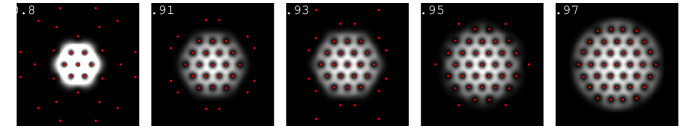
Figure 2: (Color online) Classical vortex lattice and density profile for rotation frequencies $\Omega/\omega_{\perp}=.8$, $.91$, $.93$ $.95$ and $.97$. Here $U=10$, which corresponds to $N=250$. White means high density, black low density. The vortex positions are indicated by a dot, such that also the vortices outside the condensate are visible.

From now on distances are rescaled by $\ell$, frequencies are scaled by the radial trapping frequency $\omega_{\perp}$, and we define a dimensionless interaction strength by means of

$$U=N\frac{mg^{\prime}}{4\pi\hbar^{2}}=N\frac{a}{\sqrt{2\pi}\ell_{L}}.$$ (18)

The on-site part of the energy functional can then be written as:

$$\frac{\mathcal{E}_{i}}{\hbar\omega_{\perp}N}=\frac{1}{2}\left(\omega+\frac{1}{\omega}-2\Omega\right)r^{2}n_{i}({\bf r})+2\pi\omega Un_{i}^{2}({\bf r}).$$ (19)

The lowest Landau level wavefunctions and, therefore, also the atomic density, are fully determined by the location of the vortices. To consider the quantum mechanics of the vortex lattice we, therefore, replace the functional integral over the condensate wavefunctions by a path integral over the vortex positions. This involves a non-trivial Jacobian, which does not change the results presented here, because we always consider the case that $N\gg 1$. In the calculations we take the scattering length of ⁸⁷Rb, $\lambda=700$ nm and $V_{z}/E_{z}=16$, which gives $U=25N$. The qualitative features, however, do not depend on the value of $U$.

II.3 Classical Abrikosov lattice

To determine the quadratic fluctuations around the Abrikosov lattice, we first have to find the classical groundstate. We calculated this groundstate for up to 37 vortices. The number of vortices in the condensate increases with the rotation frequency. For small numbers of vortices, the groundstate is distorted from the hexagonal lattice Aftalion05 ; Aftalion06 . In general, there are also vortices far outside the condensate. When there are more than 18 vortices in the condensate, there is generally one vortex in the center, while the other vortices order themselves in rings of multiples of six vortices. However, when a new ring of vortices enters the condensate, there is an instability towards an elliptic shape deformation. This is related to the elliptic shape deformation that occurs before a single vortex enters the condensate, and that has been investigated before theoretically Dalfovo01 ; Recati01 ; Sinha01 ; Kramer02 and has also been observed Madison01 . This shape instability plays an important role in the classical melting of the vortex lattice, as we show lateron. Pictures of the classical groundstate are given in Fig. 2 for fixed interaction $U$ and different rotation frequencies. The number of vortices within the condensate as a function of rotation frequency is plotted in Fig. 3, where we limited our study to vortex lattices that exhibit hexagonal symmetry around the origin. In the fluctuation calculation we only consider the regime where configurations consisting of one vortex in the center surrounded by rings of six vortices are stable. In that case, the coarse-grained atomic density is well approximated by a Thomas-Fermi profile Cooper04 .

\psfrag{Omega}{$\Omega$}\psfrag{N_v}{$N_{v}$}\includegraphics[scale={.66}]{fig_av.eps}

Figure 3: The number of vortices $N_{v}$ that is within the condensate as a function of the rotation frequency $\Omega$. Depending on the rotation frequency, the groundstate is either a vortex lattice with a vortex in the center surrounded by rings of a multiple of six vortices such that the number of vortices can be written as $1+6n_{r}$, or a configuration where there is no vortex in the center and the vortices order themselves in rings of multiples of three vortices, such that the total number of vortices in the condensate is a multiple of three. For $\Omega/\omega_{\perp}>.9$, the first situation is the groundstate (except for a small region, where the Bose-Einstein condensate becomes elliptically deformed) and we only calculate the fluctuations for this case. For this plot the condensate radius was defined as the radius where the angular averaged density drops below $0.003$.

II.4 Fluctuations

Next we study the quadratic fluctuations by expanding the action up to second order in the fluctuations ${\bf u}_{ni}={\bf x}_{ni}-\langle{\bf x}_{ni}\rangle$. This yields an action of the form

$$S=\sum_{i}{\bf u}_{i}\cdot({\bf T}i\partial_{t}-{\bf E})\cdot{\bf u}_{i}-t\sum_{\langle ij\rangle}{\bf u}_{i}\cdot{\bf J}\cdot{\bf u}_{j},$$ (20)

where ${\bf u}_{i}\equiv(\dots,{\bf u}_{ni},\ldots)$ is the total displacement vector of all the point vortices on site $i$. The matrices $\bf T$, $\bf E$ and $\bf J$ depend on $\Omega$, $U$, and the classical lattice positions $\langle{\bf x}_{ni}\rangle$, and are formally given by

$${\bf E}_{nm} = \left(\begin{array}[]{cc}E_{x_{ni}x_{mi}}&E_{x_{ni}y_{mi}}\\ E_{y_{ni}x_{mi}}&E_{y_{ni}y_{mi}}\end{array}\right)$$

$$= \int d^{2}{\bf r}\frac{\partial}{\partial{\bf x}_{ni}}\frac{\partial}{\partial{\bf x}_{mi}}\mathcal{E}_{i},$$

$${\bf T}_{nm} = \int d^{2}{\bf r}\frac{\partial}{\partial{\bf x}_{ni}}\frac{\partial}{\partial{\bf x}_{mi}}\mathcal{T}_{i},$$ (24)

$${\bf J}_{nm} = \int d^{2}{\bf r}\frac{\partial}{\partial{\bf x}_{ni}}\frac{\partial}{\partial{\bf x}_{mj}}\mathcal{J}_{ij}.$$

We also expand the density in the fluctuations by means of

$$n_{i}({\bf r})=\frac{n_{0}({\bf r})+\sum_{n}{\bf u}_{ni}\cdot{\bf n}_{n}({\bf r})+\sum_{nm}{\bf u}_{ni}\cdot{\bf n}_{nm}({\bf r})\cdot{\bf u}_{mi}}{1+\sum_{n}{\bf u}_{ni}\cdot{\bf n}_{ni}+\sum_{nm}{\bf u}_{ni}\cdot{\bf n}_{nm}\cdot{\bf u}_{mi}},$$ (25)

where $n_{0}({\bf r})$ is the equilibrium particle density associated with the classical lattice. We have defined the vectors

$${\bf n}_{n}({\bf r})=\left(\begin{array}[]{c}n_{x_{n}}({\bf r})\\ n_{y_{n}}({\bf r})\end{array}\right),$$ (26)

which form the dipole densities and are associated with linear variations around the classical solution, and the tensors

$${\bf n}_{nm}({\bf r})=\left(\begin{array}[]{c c}n_{x_{n}x_{m}}({\bf r})&n_{x_{n}y_{m}}({\bf r})\\ n_{y_{n}x_{m}}({\bf r})&n_{y_{n}y_{m}}({\bf r})\end{array}\right),\\$$ (27)

which form the quadrupole densities and are associated with the quadratic variations around the classical solution. Moreover,

$${\bf n}_{n}=\int d^{2}{\bf r}\;{\bf n}_{n}({\bf r})$$ (28)

and

$${\bf n}_{nm}=\int d^{2}{\bf r}\;{\bf n}_{nm}({\bf r}),$$ (29)

such that $n_{i}({\bf r})$ is always normalized to 1. The density $n_{0}({\bf r})$, and the tensors ${\bf n}_{n}({\bf r})$, ${\bf n}_{nm}({\bf r})$ are independent of time and the layer index $i$, since only the fluctuations in the vortex positions ${\bf u}_{i}(t)$ are taken as the dynamic variables. Making use of the fact that

$$n_{i}({\bf r})\propto\prod_{i}|w-w_{i}|^{2}\exp[-|w|^{2}],$$ (30)

the following expressions can be derived for the dipole density

$$n_{x_{n}}({\bf r}) = \frac{-2(x-\langle x_{ni}\rangle)}{|{\bf r}-\langle{\bf x}_{ni}\rangle|^{2}}n_{0}({\bf r}),$$ (31)

$$n_{y_{n}}({\bf r}) = \frac{-2(y-\langle y_{ni}\rangle)}{|{\bf r}-\langle{\bf x}_{ni}\rangle|^{2}}n_{0}({\bf r}).$$

For the quadrupole density for a single vortex we get

$$n_{x_{n}x_{n}}({\bf r}) = \frac{1}{|{\bf r}-\langle{\bf x}_{ni}\rangle|^{2}}n_{0}({\bf r}),$$ (32)

$$n_{x_{n}y_{n}}({\bf r}) = 0,$$

$$n_{y_{n}x_{n}}({\bf r}) = 0,$$

$$n_{y_{n}y_{n}}({\bf r}) = \frac{1}{|{\bf r}-\langle{\bf x}_{ni}\rangle|^{2}}n_{0}({\bf r}),$$

whereas for two different vortices we find

$$n_{x_{n}x_{m}}({\bf r}) = \frac{2(x-\langle x_{ni}\rangle)(x-\langle x_{mi}\rangle)}{|{\bf r}-\langle{\bf x}_{ni}\rangle|^{2}|{\bf r}-\langle{\bf x}_{mi}\rangle|^{2}}n_{0}({\bf r}),$$ (33)

$$n_{x_{n}y_{m}}({\bf r}) = \frac{2(x-\langle x_{ni}\rangle)(y-\langle y_{mi}\rangle)}{|{\bf r}-\langle{\bf x}_{ni}\rangle|^{2}|{\bf r}-\langle{\bf x}_{mi}\rangle|^{2}}n_{0}({\bf r}),$$

$$n_{y_{n}x_{m}}({\bf r}) = \frac{2(y-\langle y_{ni}\rangle)(x-\langle x_{mi}\rangle)}{|{\bf r}-\langle{\bf x}_{ni}\rangle|^{2}|{\bf r}-\langle{\bf x}_{mi}\rangle|^{2}}n_{0}({\bf r}),$$

$$n_{y_{n}y_{m}}({\bf r}) = \frac{2(y-\langle y_{ni}\rangle)(y-\langle y_{mi}\rangle)}{|{\bf r}-\langle{\bf x}_{ni}\rangle|^{2}|{\bf r}-\langle{\bf x}_{mi}\rangle|^{2}}n_{0}({\bf r}).$$

All matrices in the action for the fluctuations can be completely expressed in terms of these functions. From Eq. (19) we read off that

$${\bf E}_{nm} = \int d^{2}{\bf r}\left\{\frac{1}{2}(\omega+1/\omega-2\Omega)r^{2}\Bigl{[}({\bf n}_{n}{\bf n}_{m}-{\bf n}_{nm})n_{0}({\bf r})-\frac{1}{2}({\bf n}_{n}{\bf n}_{m}({\bf r})+{\bf n}_{m}{\bf n}_{n}({\bf r}))+{\bf n}_{nm}({\bf r})\Bigr{]}\right.$$

$$+2\pi\omega U\Bigl{[}(3{\bf n}_{n}{\bf n}_{m}-2{\bf n}_{nm}n_{0}^{2}({\bf r})-2\left({\bf n}_{n}{\bf n}_{m}({\bf r})n_{0}({\bf r})+{\bf n}_{m}{\bf n}_{n}({\bf r})n_{0}({\bf r})\right)+{\bf n}_{n}({\bf r}){\bf n}_{m}({\bf r})+2{\bf n}_{nm}({\bf r})n_{0}({\bf r})\Bigr{]}\biggr{\}}.$$

From a straightforward derivation we obtain also

$$T_{x_{n}x_{m}} = \frac{n_{y_{n}}n_{x_{m}}-n_{x_{n}}n_{y_{m}}}{4}+\frac{n_{y_{n}x_{m}}-n_{x_{n}y_{m}}}{2},$$ (35)

$$T_{x_{n}y_{m}} = \frac{n_{x_{n}}n_{x_{m}}+n_{y_{n}}n_{y_{m}}}{4}-\frac{n_{x_{n}x_{m}}+n_{y_{n}y_{m}}}{2},$$

$$T_{y_{n}x_{m}} = -T_{x_{n}y_{m}},$$

$$T_{y_{n}y_{m}} = T_{x_{n}x_{m}},$$

and

$$J_{x_{n}x_{m}} = -\frac{n_{x_{n}}n_{x_{m}}}{4}+\frac{n_{x_{n}x_{m}}+n_{y_{n}y_{m}}}{2},$$ (36)

$$J_{x_{n}y_{m}} = -\frac{n_{x_{n}}n_{y_{m}}}{4}+\frac{n_{x_{n}y_{m}}-n_{y_{n}x_{m}}}{2},$$

$$J_{y_{n}x_{m}} = -\frac{n_{y_{n}}n_{x_{m}}}{4}+\frac{n_{y_{n}x_{m}}-n_{x_{n}y_{m}}}{2},$$

$$J_{y_{n}y_{m}} = -\frac{n_{y_{n}}n_{y_{m}}}{4}+\frac{n_{x_{n}x_{m}}+n_{y_{n}y_{m}}}{2}.$$

The calculation is simplified considerably by making use of the hexagonal symmetry of the vortex lattice. Because of this symmetry the number of matrix elements to be calculated for each matrix is less then $12N_{v}^{2}+32N_{v}$ instead of $72N_{v}^{2}$, when all matrix elements are calculated independently.

II.5 Diagonalization

To diagonalize this action along the $z$ axis, we perform a Fourier transformation to obtain

$$S=\sum_{k}{\bf u}_{k}^{*}\cdot\left({\bf T}i\partial_{t}-{\bf E}-t[1-\cos(k\lambda/2){\bf J}]\right)\cdot{\bf u}_{k}.$$ (37)

Finally, we completely diagonalize this action by a transformation

$${\bf v}_{k}={\bf P}_{k}{\bf u}_{k},$$ (38)

that is normalized such that the action becomes

$$S=\sum_{k,\alpha}v_{k\alpha}^{*}(i\partial_{t}-\omega_{\alpha}(k))v_{k\alpha},$$ (39)

where $\omega_{\alpha}(k)$ are the mode frequencies of the vortex lattice. This means that the $v_{k\alpha}$, where $k$ labels the momentum in the $z$ direction and $\alpha$ labels the mode, correspond to bosonic operators with commutation relation $[v_{k\alpha},{v_{k^{\prime}\alpha^{\prime}}}^{\dagger}]=\delta_{kk^{\prime}}\delta_{\alpha\alpha^{\prime}}$. This allows us to calculate the expectation value for the fluctuations in the vortex positions, but also for the correlations between the various point vortices.

III Tkachenko modes

\psfrag{omega(k)}{$\omega(k)/\omega_{\perp}$}\psfrag{k}{$k\lambda/2$}\includegraphics[scale={.66}]{figure3}

Figure 4: Dispersion of the Tkachenko modes along the direction of the optical lattice. For this plot the parameters were chosen as: $U=10$, $t=1/10$, and $\Omega=.97$. One gapless linear mode and five gapped tight-binding-like modes can be identified. The gapless mode is the acoustic Goldstone mode associated with the broken $O(2)$-symmetry due to the presence of the vortex lattice. Note that these results were obtained in the lowest Landau level approximation, which corresponds to the compressible limit.

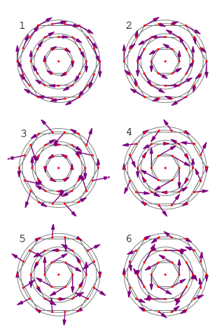
Figure 5: (Color online) Tkachenko modes. For this plot the parameters were chosen as: $U=10$, $\Omega=.97$, and $k=0$. Mode 1 is the Goldstone mode and corresponds to a pure rotation, while the modes 2-6 are gapped and ordered along increasing gap. They were previously called $s$-band modes in Ref. Coddington03 . As is visible, some of the vortices at the edge deviate from having a purely angular motion.

Figure 6: Node structure of the Tkachenko modes. The modes are ordered in the same way as in Fig. 5. Points are connected by straight lines to increase the visibility. When a wavelength is associated with the position of the nodes, it can be seen that for increasing gap the wavelength becomes shorter. This agrees qualitatively with the continuum theory of Ref. Sonin05 .

The Tkachenko modes are almost transverse modes of the vortex lattice. In a harmonic trap with cylindrical symmetry they become modes which are almost angular. In the radial direction their spectrum is discretized, because of the finite lattice size. The number of radial Tkachenko modes equals the number of rings in which the vortices have ordered themselves. For 37 vortices 6 Tkachenko modes can be identified. A close comparison with continuum theory for a finite-size system, where also a discrete spectrum was found Sonin05 , is possible but beyond the scope of this work. Moreover, the Tkachenko modes also have a dispersion in the $z$ direction. Without the optical lattice some aspects of these modes were recently investigated Chevy05 . For typical parameters this dispersion is plotted in Fig. 4, while the modes are displayed in Fig. 5. As can be seen in the latter figure, some of the vortices at the edge deviate from having a purely angular motion. As is clearly visible, there is one gapless mode, which is linear at long wavelengths, while the other modes are roughly just tight-binding-like. Moreover, various avoided crossings between these modes are clearly visible. The gapless mode is the Goldstone mode associated with the spontaneously broken rotational $O(2)$-symmetry due to the presence of the vortex lattice. When the tunneling rate is very small, the gapped modes have exactly a tight-binding dispersion and the gapless mode gets a dispersion proportional to $\sin(k\lambda/4)$. This can be understood by observing that in this case the modes are decoupled and the hamiltonian for the gapless mode reduces to the Josephson hamiltonian

$$\mathcal{H}=-E_{C}\sum_{i}\frac{\partial^{2}}{\partial\phi_{i}^{2}}+E_{J}\sum_{\langle ij\rangle}\cos(\phi_{i}-\phi_{j})^{2}.$$ (40)

Writing $p_{\phi}=-i\partial_{\phi}$, the action in momentum space thus reads after a quadratic expansion of the Josephson energy

$$\mathcal{S}=\sum_{k}\int d\omega\left(\!\begin{array}[]{c}\phi\\ p_{\phi}\end{array}\!\right)\left(\!\begin{array}[]{cc}2[1-\cos(k\lambda/2)]E_{J}&-i\omega\\ i\omega&E_{C}\end{array}\!\right)\left(\!\begin{array}[]{c}\phi\\ p_{\phi}\end{array}\!\right),$$ (41)

from which we deduce the dispersion

$$\omega^{2}(k)=2[1-\cos(k\lambda/2)]E_{J}E_{C}=4\sin^{2}(k\lambda/4)E_{J}E_{C}.$$ (42)

It is interesting to note that for a small rotation frequency, which implies a small vortex lattice, the Tkachenko modes are not the lowest-lying modes. For $U=10$, a Tkachenko mode becomes the lowest-lying gapped mode when $\Omega>0.978$, but there are many modes in between the second and the third Tkachenko mode. This confirms the expectation that increasing the vortex lattice will bring down the Tkachenko spectrum more and more.

IV Quantum melting

In this section we study vortex-lattice melting due to quantum fluctuations. We apply the Lindemann criterion to estimate the position of the melting transition. We study the influence of tunneling between the pancake condensates and compare with a local-density approximation. By looking at correlations between the vortices, we can distinguish between various phases, which are partially melted.

IV.1 Single-layer geometry

Quantum fluctuations of the vortices ultimately result in melting of the vortex lattice. To decide whether or not the lattice is melted, we use the Lindemann criterion, which in this inhomogeneous situation has to be applied locally. The Lindemann criterion means that the lattice is melted, when

$$\frac{\langle{\bf u}_{ni}^{2}\rangle}{\Delta_{ni}^{2}}>c_{L}^{2},$$ (43)

where $\Delta_{ni}$ is average distance to the neighboring vortices. The critical value $c_{L}$, is known as the Lindemann parameter. This parameter is a priori unknown, but values found from comparison with Monte Carlo simulations are typically in the range $c_{L}=0.1-0.3$. The value $c_{L}=0.1$ was recently found from elaborate calculations for a triangular vortex lattice in high-$T_{c}$ superconductors, which also compared well to experiments in that case Dietel05 . We, therefore, use this value in our calculations. Note that the results we obtain depend quantitatively on the value of the Lindemann parameter. Changing this value shifts the curves, but the qualitative features remain the same.

Due to the inhomogeneity of our system, we have to apply this criterion locally. Because the coarse-grained particle density decreases with the distance to the origin, vortices on the outside are already melted, while the inner part of the crystal remains solid Fischer04 . Therefore, a crystal phase in the inside coexists with a liquid phase on the outside. In Fig. 7 we compute the radius of the crystal phase $R_{\rm cr}$ normalized to the condensate radius $R$, as a function of the rotation frequency for fixed a number of particles and a fixed interaction strength $U$, but for various hopping strengths $t$. Also here we define the condensate radius $R$ as the radius for which the angularly averaged density drops below $0.003$. The crystal radius $R_{\rm cr}$ is defined as the radius of the innermost ring of vortices that is melted according to the Lindemann criterion. When according to this definition $R_{\rm cr}>R$, we set the crystal radius equal to the condensate radius, i.e., $R_{\rm cr}=R$.

\psfrag{N_v}{$N_{v}$}\psfrag{Omega}{$\Omega/\omega_{\perp}$}\psfrag{R_cr/R}{ $R_{\rm cr}/R$}\includegraphics[scale={.66}]{figure_melt}

Figure 7: Crystal radius $R_{\rm cr}$ normalized to the condensate radius $R$ as a function of the rotation frequency for $N=250$ and $U=10$. The solid line is for $t=0$ and the dashed lines are for $t=1/1000$ and $1/100$ (from left to right). The dotted lines are the result of the local-density approximation, where for the upper curve we took the criterion $N/N_{v}=6$ and for the lower curve $N/N_{v}=8$. In all the figures in this paper we have connected the points by straight lines. Due to the finite numerical resolution the jump between the plateau’s appears therefore not vertical.

The ratio $R_{\rm cr}/R$ shows discrete steps because of the ring-like structure in which the vortices order themselves.

IV.2 Local-density approximation

We compare this with a simple local density calculation, where the criterion $N/N_{v}=n(r)/n_{v}(r)=6$ Cooper01 or $N/N_{v}=n(r)/n_{v}(r)=8$ Sinova02 is applied locally, by making use of a Thomas-Fermi density profile to describe the coarse-grained atomic density. Substituting the Thomas-Fermi profile

$$n_{\rm TF}(r)=\frac{2}{\pi R_{\rm TF}^{2}}\left(1-\frac{r^{2}}{R_{\rm TF}^{2}}\right),$$ (44)

where $R_{\rm TF}$ is the Thomas-Fermi radius, in the on-site energy in Eq. (19), we obtain

$$\left(\omega+\frac{1}{\omega}-2\Omega\right)\frac{R_{\rm TF}^{2}}{6}+\frac{\beta 8\omega U}{3R_{\rm TF}^{2}}.$$

We have introduced here also the Abrikosov parameter $\beta={\int n^{2}({\bf r})}/{(\int n({\bf r}))^{2}}\simeq 1.1596$ for the hexagonal lattice. Minimizing for $R_{\rm TF}$ gives

$$R_{\rm TF}^{4}=\frac{16\beta U\omega^{2}}{1+\omega^{2}-2\omega\Omega},$$ (45)

which on substitution gives for the on-site energy

$$\frac{4}{3}\sqrt{\beta U}\sqrt{1+\omega^{2}-2\omega\Omega}.$$

This is minimized for

$$\omega=\Omega,$$ (46)

which sets the variational parameter $\ell$. The Thomas-Fermi radius is then given by

$$R_{\rm TF}^{4}=16\frac{\Omega^{2}\beta U}{1-\Omega^{2}}.$$ (47)

In lowest order the vortex density is given by

$$n_{v}({\bf r})=\frac{1}{\pi\ell^{2}}.$$ (48)

Solving now

$$\nu({\bf r})=\frac{n({\bf r})}{n_{v}({\bf r})}=\nu_{c},$$ (49)

we get for the crystal radius normalized to the Thomas Fermi radius the result

$$\frac{R_{\rm cr}}{R_{\rm TF}}=\sqrt{1-\frac{\nu_{c}R^{2}}{2N}}=\sqrt{1-\frac{2\nu_{c}}{N}\sqrt{\frac{\Omega^{2}\beta U}{(1-\Omega^{2})}}}.$$ (50)

For comparison this line is plotted in Fig. 7. As can be seen there are important finite-size corrections to the local-density approximation. The local-density approximation fails to take into account the discrete nature of the vortex positions. Moreover, it predicts the total melting of the crystal at considerable higher rotation frequencies than the exact answer.

In principle there are corrections to the vortex density due to the Thomas-Fermi profile of the particle density. A better approximation near the center of the trap is Ho01

$$n_{v}(r)=\frac{1}{\pi\ell^{2}}-\frac{1}{\pi R_{\rm TF}^{2}}\frac{1}{(1-r^{2}/R_{\rm TF}^{2})^{2}}.$$ (51)

However, this vortex density becomes zero well within the Thomas-Fermi radius. As a result the ratio $n({\bf r})/n_{v}({\bf r})$ diverges and is always bigger than 8. Higher-order contributes should be taken into account to solve this problem. Instead we compare with the constant vortex density

$$n_{v}(r)=\frac{1}{\pi\ell^{2}}-\frac{1}{\pi R_{\rm TF}^{2}},$$ (52)

which corresponds to a Gaussian distribution of the atomic density with radius $R_{\rm TF}$. Straightforward derivation gives then

$$\frac{R_{\rm cr}}{R_{\rm TF}} = \sqrt{1-\frac{\nu_{c}(R^{2}-1)}{2N}}$$ (53)

$$= \sqrt{1-\frac{2\nu_{c}}{N}\left(\sqrt{\frac{\Omega^{2}\beta U}{(1-\Omega^{2})}}-1\right)}.$$ (54)

This shifts the curves for the local-density theory in Fig. 7 a little bit upwards, and makes the comparison even less favourable.

IV.3 Multi-layer geometry

When the tunneling between pancakes is turned on, the fluctuations are also coupled in the axial direction. This decreases the fluctuations in the vortex displacements because the stiffness of the vortices increases. Hence melting occurs for higher rotation frequencies, as is visible in Fig. 7. In Fig. 8 we show the crystal radius for fixed rotation frequency and increasing hopping amplitude.

\psfrag{t}{$t$}\psfrag{R_cr/R}{ $R_{\rm cr}/R$}\includegraphics[scale={.66}]{figure_freezing}

Figure 8: Crystal radius $R_{\rm cr}$ normalized to the condensate radius $R$ as a function of the hopping amplitude $t$ for $N=250$, $U=10$ and $\Omega=.96$.

\psfrag{exp}{$e^{-\langle({\bf u}_{ni}-{\bf u}_{nj})^{2}\rangle}$}\psfrag{z}{$2z/\lambda$}\psfrag{t}{$t$}\includegraphics[scale={.66}]{figure_corr}

Figure 9: Axial correlation function $e^{-\langle({\bf q}\cdot({\bf u}_{ni}-{\bf u}_{nj}))^{2}\rangle/2}$ as a function of the distance along the axial direction for ${\bf q}=(1/\ell,1/\ell)$, $N=250$, $U=10$, and $\Omega=0.97$. The various curves have, from top to bottom, a hopping parameter $t=10^{-2}$, $t=10^{-3}$, $t=10^{-4}$, $t=10^{-5}$, and $t=10^{-6}$, respectively. The correlation function decays as a power law and in the inset the power is plotted as a function of the hopping amplitude $t$. The power thus scales with $1/\sqrt{t}$.

To determine the presence of crystalline order in the axial direction, we calculate the correlation function

$$\langle e^{i{\bf q}\cdot({\bf u}_{ni}-{\bf u}_{nj})}\rangle,$$

which is related to the static structure factor. For our gaussian theory, this reduces to

$$e^{-\langle[{\bf q}\cdot({\bf u}_{ni}-{\bf u}_{nj})]^{2}\rangle/2}.$$

For the central vortex the correlation function $\langle{\bf u}_{0i}{\bf u}_{0j}\rangle$ decays exponentially, which signals long-range order. For the other vortices $\langle[{\bf q}\cdot({\bf u}_{ni}-{\bf u}_{nj})]^{2}\rangle$ grows as a logarithm, such that $e^{-\langle[{\bf q}\cdot({\bf u}_{ni}-{\bf u}_{nj})]^{2}\rangle}$ decays algebraically. This is in agreement with the expectation for a one-dimensional system at zero temperature. In Fig. 9 we show the axial correlation function for one of the vortices outside the center.

Since the lattice spacing $\lambda/2$ is the only length scale in the $z$ direction, it also determines the axial correlation length. The power of the algebraic decay scales with $1/\sqrt{t}$. This can be understood when we assume that the gapless Tkachenko mode gives the dominant contribution to the axial correlation. Using the effective hamiltonian for this mode from Eq. (40), we obtain the following expression:

$$\langle({\bf u}_{in}-{\bf u}_{jn})^{2}\rangle\simeq\frac{r_{n}^{2}}{\sqrt{E_{J}E_{C}}}\times$$ (55)

$$\frac{2}{\pi}\int_{0}^{\pi}dk\sin^{2}(k(i-j)/2))\left(\frac{E_{C}}{\sin(k/2)}+E_{J}\sin(k/2)\right),$$

where we rescaled $k$ , in units of the lattice spacing $\lambda/2$, $r_{n}$ is the distance of the vortex to the origin and we used that $1-\cos(k(i-j))=2\sin^{2}(k(i-j)/2)$. Only the first term in the brackets is divergent for $k\rightarrow 0$, so we neglect the second term. We make the approximation $\sin(k/2)\simeq k/2$. When $i-j$ is large we can approximate the rapidly oscillating function $\sin^{2}(k(i-j)/2)$ by its average $1/2$, except for a region near $k=0$. We obtain then

$$\frac{4r_{n}^{2}}{\pi}\sqrt{\frac{E_{C}}{E_{J}}}\int_{0}^{\pi}dk\frac{\sin^{2}(k(i-j)/2)}{k}$$ (56)

$$=\frac{4r_{n}^{2}}{\pi}\sqrt{\frac{E_{C}}{E_{K}}}\left(\int_{0}^{\tfrac{4\pi}{i-j}}dk\frac{\sin^{2}(k(i-j)/2)}{k}+\frac{1}{2}\int_{\tfrac{4\pi}{i-j}}^{\pi}\frac{1}{k}\right)$$

$$=\frac{4r_{n}^{2}}{\pi}\sqrt{\frac{E_{C}}{E_{J}}}\left(\int_{0}^{4\pi}dk\frac{\sin^{2}}{k}+\frac{1}{2}\log 4(i-j)\right)$$

$$=\frac{2r_{n}^{2}}{\pi}\sqrt{\frac{E_{C}}{E_{J}}}\left(\log 4(i-j)+C_{1}\right),$$

where the constant $C_{1}=\gamma+\log(8\pi)+{\rm Ci}(8\pi)\simeq 3.80296$. Using now the fact that $E_{J}\propto t$, we conclude that indeed the power of the algebraic decay of $e^{-\langle({\bf q}\cdot({\bf u}_{ni}-{\bf u}_{nj}))^{2}\rangle/2}$ scales with $1/\sqrt{t}$.

For nonzero temperatures we obtain a linear rise of the correlation function $\langle({\bf u}_{ni}-{\bf u}_{nj})^{2}\rangle$, which can be understood from the same argument, since then we have to add the Bose-Einstein distribution, which for very low temperatures can be approximated by

$$\frac{1}{e^{\omega(k)/k_{B}T}-1}\simeq\frac{k_{B}T}{\omega(k)}=\frac{k_{B}T}{2\sqrt{E_{J}E_{C}}\sin(k\lambda/4)}.$$ (57)

When we again rescale the momentum by the lattice constant $\lambda/2$ and approximate $\sin k/2\simeq k/2$, we observe that the $1/k$-factor in the intergrand of Eq. (56) is replaced by $1/k^{2}$. This gives that up to a constant $\langle({\bf u}_{in}-{\bf u}_{jn})^{2}\rangle\propto i-j$ and $e^{-\langle({\bf q}\cdot({\bf u}_{ni}-{\bf u}_{nj}))^{2}\rangle/2}$ decays exponentially.

IV.4 Correlations

Melting for small arrays of electrons in quantum dots that are composed of two or three shells Bedanov94 ; Schweigert95 ; Belousov98 ; Filinov01 , and of vortex lattice shells Lozovik98 ; Pogosov06 is predicted to occur in two stages. First the oriental order between different shells is destroyed, while after that the radial order is destroyed. We also find this behavior for the vortex lattice. For that we compute the correlation function between various vortices and decompose it in radial and angular fluctuations. A shell structure is found, where vortices with almost (but not necessarily exactly) the same distance group together. Between these shells angular fluctuations dominate, while within the shell angular fluctuations are suppressed and radial fluctuations dominate. This can be understood if we assume that the Tkachenko modes dominate the fluctuations, because they leave the rings intact, but change the relative angle between the rings.

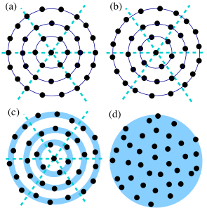
Figure 10: (Color online) Phases that can be distinguished by looking to radial and angular correlations between vortices on the same and on different shells: a) a solid, b) a solid of solid shells, c) a hexatic liquid, d) a liquid.

To quantify this, we introduce the following order parameter to measure fluctuations in the relative angle of neighboring shells

$$\Gamma_{nm}^{\rm SS}=\left(\frac{{\bf u}_{ni}^{\rm ang}}{r_{n}}-\frac{{\bf u}_{mi}^{\rm ang}}{r_{m}}\right)^{2},$$ (58)

for neighboring vortices $n$ and $m$ on different shells, where $r_{n}$ is the distance of vortex $n$ to the origin and only the angular part of the fluctuations in the displacement field is considered. Let $N_{v}^{\rm max}$ be the maximum number of vortices on either of the two shells. The shells are decoupled with respect to each other if

$$\Gamma_{nm}^{\rm SS}>\frac{2\pi}{N_{v}^{\rm max}}c_{L}^{2},$$ (59)

with $c_{L}=0.1$ the same Lindemann parameter. Furthermore we introduce the correlation function

$$\Gamma_{nm}=\frac{\langle({\bf u}_{ni}-{\bf u}_{mi})^{2}\rangle}{2\Delta_{mn}^{2}},$$ (60)

where $\Delta_{mn}$ is the distance between the neighboring vortices $m$ and $n$ and we split this up in a radial and angular component. Moreover we distinguish between the case when $n$ and $m$ are on the same shell, which we denote by $\Gamma_{r}^{\rm rad}$ and $\Gamma_{r}^{\rm ang}$, or on different shells, denoted by $\Gamma_{rr^{\prime}}^{\rm rad}$ and $\Gamma_{rr^{\prime}}^{\rm ang}$. We use the definition that order is destroyed if the order parameters exceeds the Lindemann parameter, i.e., $\Gamma>c_{L}^{2}=0.01$. When the fluctuations are small, the vortex lattice is in the crystal phase. This phase is defined as $\Gamma_{nm}=\Gamma_{nm}^{\rm rad}+\Gamma_{nm}^{\rm ang}<c_{L}^{2}$, for $n$ and $m$ on the same shell and on different shells. In particular, there is positional order of the radii of the different shells. However, we can distinguish between the case that there exists oriental order between the shells, in which case the relative angle is locked and $\Gamma_{nm}^{\rm SS}<\frac{2\pi}{N_{v}^{\rm max}}c_{L}^{2}$. This we call the solid phase (S). When the oriental order between the shells is destroyed we call this phase the solid of solid shells (SS). The melted phase is charactarized by $\Gamma_{nm}=\Gamma_{nm}^{\rm rad}+\Gamma_{nm}^{\rm ang}>c_{L}^{2}$, and in particular the positional order in the radii of the different shells is destroyed. Within this phase it is still possible to have a well-defined angle between vortices on the same shell, i.e., $\Gamma_{r}^{\rm ang}<c_{L}^{2}$. This we call the hexatic liquid (HL), whereas when this order is destroyed we call it the liquid (L). These phases are schematically indicated in Fig. 10.

These criteria should again be applied locally because of the inhomogeneous density, and we define the phase boundaries in analogy to the previous definition as the radius of the innermost ring that is partly melted. For our parameters it turns out that the angle between neighboring vortices on the same ring is always well-defined, but we can identify the transition between the solid, the solid of solid shells, and the hexatic liquid. The result of this calculation is presented in Fig. 11. In agreement with known theory for vortex lattices, the hexatic symmetry is a very robust phenomenon.

\psfrag{Omega}{$\Omega/\omega_{\perp}$}\psfrag{R_Gamma/R}{ $R_{\Gamma}/R$}\includegraphics[scale={.66}]{melting2}

Figure 11: Phase boundaries between the solid (S), the solid of solid shells (SS), and the hexatic liquid (HL) as a function of radial distance and rotation frequency for $N=250$ and $U=10$. The solid line is for $t=0$ and the dashed line is for $t=1/100$.

V Classical melting

The Bose-Einstein temperature for a two-dimensional noninteracting Bose gas in a harmonic trap is given by

$$k_{B}T_{c}=\omega_{\perp}\sqrt{\zeta(2)/N},$$ (61)

where $\zeta(x)$ is the Riemann zeta function and $\zeta(2)\simeq 1.28$. When the temperatures are much lower than this temperature, there is no thermal cloud present in the gas and we can easily extend our analysis to this regime. This is experimentally relevant, because the zero-temperature limit is difficult to reach Cornell . However, according to the Mermin-Wagner theorem, a two-dimensional crystal cannot exist for nonzero temperatures. For an infinite hexagonal vortex lattice this can be seen as follows. Let ${\bf u}({\bf x},t)$ be the displacement field of the vortex lattice. We define

$$u_{L}({\bf q},t) = (q_{x}u_{x}({\bf q},t)+q_{y}u_{y}({\bf q},t))/q,$$ (62)

$$u_{T}({\bf q},t) = (q_{x}u_{y}({\bf q},t)-q_{y}u_{x}({\bf q},t))/q,$$ (63)

as the longitudinal and transverse fluctuations in the displacement field, respectively. For long wavelengths the action for the vortex lattice is then given by

$$S=\int dt\int\frac{d^{2}{\bf q}}{(2\pi)^{2}}\;\left(\bar{n}\;u_{L}\hbar\partial_{t}u_{T}-c_{1}q^{2}|u_{L}|^{2}-c_{66}q^{2}|u_{T}|^{2}\right),$$ (64)

where $\bar{n}$ is the average atomic density and $c_{1}$ and $c_{66}$ are the compressional modulus and the shear modulus of the vortex lattice, respectively. We have used that the vortex-vortex interaction decays faster than $1/r^{2}$, since the condensate is assumed to be weakly interacting. From this action we read off that the dispersion of the (almost transverse) Tkachenko mode is quadratic, i.e.,

$$\omega({\bf q})=2\sqrt{c_{1}c_{66}}q^{2}/\bar{n}.$$ (65)

The fluctuations in the vortex positions can then be calculated as

$$\langle u^{2}\rangle=\int\frac{d^{2}{\bf q}}{(2\pi)^{2}}\frac{1}{2\bar{n}}\left(\sqrt{\frac{c_{1}}{c_{66}}}+\sqrt{\frac{c_{66}}{c_{1}}}\right),$$ (66)

which is a converging integral if we realize that the integration is over the first Brillouin zone. However, for nonzero temperature, we have to add the Bose-Einstein distribution $1/(e^{\beta\omega(k)}-1$), which for long wavelengths can be approximated by $k_{B}T/\omega(k)$. The temperature fluctuations are therefore given by

$$\langle u^{2}\rangle_{T}=k_{B}T\int\frac{d^{2}{\bf q}}{(2\pi)^{2}}\frac{1}{2\bar{n}q^{2}}\left(\frac{1}{c_{1}}+\frac{1}{c_{2}}\right),$$ (67)

which diverges logarithmically in the infrared. Therefore, the usual Lindemann criterion always predicts melting for infinite isolated two-dimensional vortex lattices. For a finite system there is a natural infrared cut-off of the divergence, but still there are large contributions from low-lying modes. Any finite amount of tunneling, however, will turn the system into a three-dimensional system, where the Mermin-Wagner theorem does not apply any more. If $k$ denotes the momentum in the $z$ direction, we can then define

$$u_{L}({\bf q},k,t) = (q_{x}u_{x}({\bf q},k,t)+q_{y}u_{y}({\bf q},k,t)/q,$$ (68)

$$u_{T}({\bf q},k,t) = (q_{x}u_{y}({\bf q},k,t)-q_{y}u_{x}({\bf q},k,t))/q.$$ (69)

Tunneling results in an additional term in the action that for long wavelengths is given by

$$\int dt\int\frac{dk}{2\pi}\int\frac{d^{2}{\bf q}}{(2\pi)^{2}}\;Jk^{2}(|u_{L}|^{2}+|u_{T}|^{2}),$$

where $J$ is an effective hopping parameter. This still gives a quadratic dispersion, but with an anisotropic mass, i.e.,

$$\omega({\bf q},k)=2\sqrt{(c_{1}q^{2}+Jk^{2})(c_{66}q^{2}+Jk^{2})}/\bar{n}.$$ (70)

Writing ${\bf p}=(q_{x},q_{y},k)$ and using spherical coordinates the dispersion becomes

$$\omega({\bf p})=2p^{2}\sqrt{(c_{1}\sin^{2}\theta+J\cos^{2}\theta)(c_{66}\sin^{2}\theta+J\cos^{2}\theta)}/\bar{n}.$$ (71)

The fluctuations can therefore be calculated as

$$\langle u^{2}\rangle_{T}=k_{B}T\int\frac{dpd\phi}{(2\pi)^{2}}\frac{p^{2}\sin\theta}{2\bar{n}p^{2}}\times$$ (72)

$$\left\{\frac{1}{\sqrt{(c_{1}\sin^{2}\theta+J\cos^{2}\theta)(c_{66}\sin^{2}\theta+J\cos^{2}\theta)}}\times\right.$$

$$\left.\left(\sqrt{\frac{c_{1}\sin^{2}\theta+J\cos^{2}\theta}{c_{66}\sin^{2}\theta+J\cos^{2}\theta}}+\sqrt{\frac{c_{66}\sin^{2}\theta+J\cos^{2}\theta}{c_{1}\sin^{2}\theta+J\cos^{2}\theta}}\right)\right\}.$$

which clearly converges in the infrared and the fluctuations remain finite. For a system of coupled pancake Bose-Einstein condensates we can therefore still use the usual Lindemann criterion.

In Fig. 12 the vortex-crystal radius is plotted as a function of the rotation frequency for a fixed and strong tunneling and various temperatures. In the regime $\Omega/\omega_{\perp}\in[.938,.941]$ there is a dynamical instability towards elliptic shape deformation. This is indicated by a shaded region in the plotted figures. We did not calculate the fluctuations in this regime. This is related to the elliptic shape deformation that occurs before a single vortex enters the condensate, and that has been investigated before theoretically Dalfovo01 ; Recati01 ; Sinha01 ; Kramer02 and has also been observed Madison01 . Because the unstable mode crosses zero, this causes huge fluctuations in the neighborhood of this instability.

\psfrag{Omega}{$\Omega/\omega_{\perp}$}\psfrag{R_cr}{ $R_{\rm cr}/R$}\psfrag{omega}{ $\omega(\Omega)$}\includegraphics[scale={.66}]{fig_melt_temp}

Figure 12: Crystal radius $R_{\rm cr}$ normalized to the condensate radius $R$ as a function of the rotation frequency for $N=250$, $U=10$, $t=1/20$, and $T=T_{c}/40$ (dotted line), $T=T_{c}/50$ (dashed line), and $T=T_{c}/100$ (solid line). In the shaded region there is a dynamical instability towards elleptic shape deformation. In the inset the frequency of the unstable mode is plotted.

In Fig. 13 we calculate the temperature for which quantum fluctuations of the vortex crystal are equal to the temperature fluctuations, which defines the crossover temperature between quantum and classical melting. The temperature should be chosen much lower to observe the effects of quantum melting.

\psfrag{T_cross}{$T_{c}/T_{\rm cross}$}\psfrag{Omega}{$\Omega/\omega_{\perp}$}\includegraphics[scale={.66}]{fig_crosstemp}

Figure 13: Inverse of the crossover temperature $T_{\rm cross}$ a function of $\Omega/\omega_{\perp}$ for $N=250$ and $U=10$. Lines are for $t=1/20$ (solid line) and $t=0$ (dashed line). As in Fig. 12, the shaded region is excluded because of the presence of a dynamical instability.

In Fig. 14 the vortex-crystal radius is plotted as a function of temperature for a fixed rotation frequency.

\psfrag{T_c/T}{$T_{c}/T$}\psfrag{R_cr}{ $R_{\rm cr}/R$}\includegraphics[scale={.66}]{fig_temp}

Figure 14: Crystal radius $R_{\rm cr}$ normalized to the condensate radius $R$ as a function of $T_{c}/T$ for $N=250$, $U=10$, and $\Omega/\omega_{\perp}=0.93$. From left to right the lines have hopping parameter $t=1$, $t=0.1$, $t=0.05$, and $t=0.01$, respectively.

\psfrag{Omega}{$\Omega/\omega_{\perp}$}\psfrag{R_Gamma/R}{ $R_{\Gamma}/R$}\includegraphics[scale={.66}]{hexaticT_20}

\psfrag{Omega}{$\Omega/\omega_{\perp}$}\psfrag{R_Gamma/R}{ $R_{\Gamma}/R$}\includegraphics[scale={.66}]{hexaticT_35}

\psfrag{Omega}{$\Omega/\omega_{\perp}$}\psfrag{R_Gamma/R}{ $R_{\Gamma}/R$}\includegraphics[scale={.66}]{hexaticT_100}

Figure 15: Phase boundaries between the solid of solid shells (SS), hexatic liquid (HL) and liquid (L), as a function of radial distance and rotation frequency for $N=250$, $U=10$, and $t=0$ (dashed line) and $t=1/20$ (solid lines). The figures are for a) $T=T_{c}/20$, b) $T=T_{c}/35$, and c) $T=T_{c}/100$.

When tunneling between sites is suppressed, the correlation between neighboring vortices

$$\frac{\langle({\bf u}_{in}-{\bf u}_{im})^{2}\rangle}{2\Delta_{mn}^{2}},$$ (73)

where $\Delta_{mn}$ is the distance between the vortex $n$ and $m$ at site $i$, has been proposed as an appropriate order parameter, with unchanged Lindemann parameter Zahn99 ; Baym04 ; Kierfeld04 ; Dietel06 . In this order parameter the diverging small momentum contributions are subtracted. Nevertheless, it turns out that we have to go to low temperatures to see any crystalline order. The same phases as in the case of zero temperature can be distinguished. The result of this calculation is plotted in Fig. 15. Note that a true solid phase of the vortex lattice is not observable in these phase diagrams, not even for the lowest temperature of $T=T_{c}/100$.

VI Anharmonic radial confinement

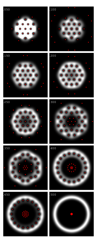
Figure 16: (Color online) Classical vortex lattice and density profile for rotation frequencies $\Omega/\omega_{\perp}=1.05,1.1,\ldots,1.5$ in the presence of a quartic potential. Parameters are chosen as $U=10$ and $\lambda=0.01$. White means high density, black low density. The vortex positions are indicated by a dot, such that also the vortices outside the condensate are visible.

\psfrag{Omega}{$\Omega/\omega_{\perp}$}\psfrag{R}{ $R$}\includegraphics[scale={.66}]{fig_radii}

Figure 17: Inner and outer radius of the condensate as a function of the rotation frequency for $N=250$, $U=10$, $\lambda=0.01$, and $t=0$. The solid line is the result of a calculation using the lowest Landau approximation and with 37 vortices taken into account. The dashed line is the result of the approximation that the density profile is described by a quartic polynomial.

The inclusion of a quartic potential, in addition to the usual harmonic potential, has attracted interest for several reasons. The quartic potential plays an important role in the understanding of vortex nucleation Fetter01 ; Gosh04 . For our purposes, however, it is more important that in this way rotation frequencies larger than the trap frequency can be applied. This causes the density to be lower in the center of the trap, and eventually gives rise to the formation of giant vortices, i.e., multiple quantized vortices, in the center of the trap Lundh02 ; Kasamatsu02 ; Kavoulakis03 . Experiments in this setup were performed and it was observed that the vortex lattice became disordered, but no giant vortex was observed Bretin04 . Giant vortex formation was observed by artificially removing the inner part of a fast rotating condensate by means of a laser beam Engels02 . Shape oscillations of a vortex lattice in an anharmonic potential were also studied experimentally Stock04 . Theoretically, the phase diagram of this system was studied intensively to identify the parameter space where giant vortex formation can take place Aftalion04 ; Jackson04 ; Fetter04 . Other aspects that are studied are the dynamics of forming the giant vortex Tsubota03 ; Fu05 , oscillations of the vortex lattice Cozzini05 , aspects on observation Danaila05 ; Cozzini06 , and stability of quantum fluctuations Kim05 .

It is straightforward to extend our analysis to this case. We first of all add the quartic potential

$$V_{4}(r)=\lambda\frac{r^{4}}{\ell_{\perp}^{4}},$$ (74)

where $\ell_{\perp}$ is the harmonic length associated with the radial trapping. We again use lowest Landau level wavefunctions and make the ansatz that there is one vortex in the center and that the rest of the vortices order themselves in rings of multiples of six. The resulting density profiles for 37 vortices are plotted in Fig. 16 as a function of the rotation frequency. We compare these density profiles with the Thomas-Fermi-like density profiles of the form

$$n(r)\propto\left(\frac{r^{2}}{R_{1}^{2}}\pm 1\right)\left(\frac{r^{2}}{R_{2}^{2}}-1\right),$$ (75)

that come from minimizing the on-site energy functional without paying attention to the lowest Landau level constraint. When the minus sign is chosen there appears a hole in the density, and the condensate shape is annular with inner radius $R_{1}$ and outer radius $R_{2}$. We compare the values coming from this ansatz with the inner and outer radius coming from the lowest Landau level densities in Fig. 17. They agree quite well.

We also calculate the quantum fluctuations of the vortices. This is only possible in a limited regime, where the ansatz of a central vortex surrounded by rings of six vortices is dynamically stable. In this regime, the inner part of the vortex crystal is melted, although the particle density is nonzero there. We define the liquid radius $R_{\rm L}$ as the radius of the innermost vortex that is part of the vortex crystal. In the region $\Omega/\omega_{\perp}\in[1.155,1.25]$ the ansatz is stable against fluctuations. We find that the liquid radius in this region is almost constant and given by $R_{\rm L}/R\simeq.58$. There is a second radius which separates the vortex crystal from the vortex liquid that is at the outside of the condensate, which corresponds to the crystal radius $R_{\rm cr}$ defined before. In this region this radius is always equal to the condensate radius or $R_{\rm cr}/R=1.0$.

VII Conclusions and outlook

In this article we derived the theory of vortex fluctuations in a one-dimensional optical lattice. We showed that in this configuration the modes of the vortex lattice get a dispersion in the axial direction. In particular we discussed the Bloch bands of the Tkachenko modes. Based on the Lindemann criterion we studied the melting of the vortex lattice. Because of the inhomogeneous density the melting occurs from the outside inwards. Comparison with a local density-approximation yields important finite-size corrections, because the local-density theory does not take into account the discrete nature of the vortices and overestimates the rotation frequency that is needed for total melting of the vortex lattice. Tunneling between the sites of the optical lattices decreases the fluctuations and causes freezing of the vortex lattice. Temperatures on the other hand increases the fluctuations considerably. The crossover temperature from classical to thermal melting is very low, which makes it an experimentally difficult problem to see the effects of quantum fluctuations. By looking into the correlations between the vortices, several phases can be distinguished, where part of the order is destroyed by quantum fluctuations.

In the one-dimensional optical lattice there is a clear experimental signal for both the fluctuations in the vortex position and the liquid. The fluctuations can be measured in analogy with the situation of a single vortex in an optical lattice. By imaging in axial direction one will see the vortex cores distributed themselves in a gaussian distribution around their equilibrium position, from which the size of the fluctuations can be extracted Martikainen04 . In the liquid the vortices are no longer individually visible, which is a clear distinction from the vortex crystal. An interesting question is whether the liquid will completely restore the rotation symmetry that is broken by the presence of the vortex lattice, or the liquid is partly pinned because of the interaction between the vortex liquid and the vortex crystal.

It remains a challenging problem to describe the coexisting crystal-liquid. This will allow to decide on the occurrence of melting based on energy considerations and thus shed more light on the accuracy of the application of the Lindemann criterion in this inhomogeneous situation. This also applies to the phases where partial melting takes place. It is not only important to find a good description of these phases themselves, but also the predicted phase coexistence between them raises interesting new questions.

References

- (1) M. R. Matthews, B. P. Anderson, P.C. Haljan, D.S. Hall, C.E. Wieman and E.A. Cornell, Phys. Rev. Lett. 83, 2498 (1999).
- (2) K. W. Madison, F. Chevry, W. Wohlleben and J. Dalibard, Phys. Rev. Lett. 84, 806 (2000).
- (3) A. Fetter and A. Svidzinsky, J. Phys.: Condens. Matter 13, R135 (2001).
- (4) E. Hodby, O.M. Maragò, G. Hechenblaikner, and C.J. Foot, Phys. Rev. Lett. 86, 2196 (2002).
- (5) E. Hodby, G. Hechenblaikner, S.A. Hopkins, O. M. Maragò and C.J. Foot, Phys. Rev. Lett. 88, 010405 (2002).
- (6) P. Rosenbusch, V. Bretin, and J. Dalibard, Phys. Rev. Lett. 89, 200403 (2002).
- (7) A. E. Leanhardt, A. Görlitz, A. P. Chikkatur, D. Kielpinski, Y. Shin, D. E. Pritchard, and W. Ketterle, Phys. Rev. Lett. 89, 190403 (2002).
- (8) A. E. Leanhardt, Y. Shin, D. Kielpinski, D. E. Pritchard, and W. Ketterle, Phys. Rev. Lett. 90, 140403 (2003)
- (9) J.R. Abo-Shaeer, J. M. Vogels, and W. Ketterle, Science 292, 467 (2001).
- (10) J. R. Abo-Shaeer, C. Raman, and W. Ketterle, Phys. Rev. Lett. 88, 070409 (2002).
- (11) P. Engels, I. Coddington, P. C. Haljan, and E. A. Cornell, Phys. Rev. Lett. 89, 100403 (2002).
- (12) P. Engels, I. Coddington, P. C. Haljan, V. Schweikhard, and E. A. Cornell Phys. Rev. Lett. 90, 170405 (2003)
- (13) I. Coddington, P. Engels, V. Schweikhard, and E. A. Cornell, Phys. Rev. Lett. 91, 100402 (2003).
- (14) V. Schweikhard,1 I. Coddington, P. Engels, V. P. Mogendorff, and E. A. Cornell, Phys. Rev. Lett. 92, 040404 (2004).
- (15) V. Bretin, S. Stock, Y. Seurin, and J. Dalibard, Phys. Rev. Lett. 92, 050403 (2004).
- (16) N.K. Wilkin, J.M.F. Gunn, and R.A. Smith, Phys. Rev. Lett. 80, 2265 (1998);
- (17) N.R. Cooper and N.K. Wilkin, Phys. Rev. B 60, R16279 (1999).
- (18) N.K. Wilkin and J.M.F. Gunn, Phys. Rev. Lett. 84, 6 (2000).
- (19) N.R. Cooper, N.K. Wilkin, and J.M.F. Gunn, Phys. Rev. Lett. 87, 120405 (2001).
- (20) T.-L. Ho and E.J. Mueller, Phys. Rev. Lett. 89, 050401 (2002).
- (21) B. Paredes, P. Zoller, and J.I. Cirac, Phys. Rev. A 66, 033609 (2002).
- (22) N. Regnault and Th. Jolicoeur, Phys. Rev. Lett. 91, 030402 (2003).
- (23) R. B. Laughlin, Phys. Rev. Lett. 50, 1395 (1983).
- (24) G. Moore and N. Read, Nucl. Phys. B 360, 362 (1991).
- (25) N. Read and E. Rezayi, Phys. Rev. B 59, 8084 (1999).
- (26) E.H. Rezayi, N. Read, and N.R. Cooper, Phys. Rev. Lett. 95, 160404 (2005).
- (27) D. Jaksch, C. Bruder, J. I. Cirac, C. W. Gardiner, and P. Zoller, Phys. Rev. Lett. 81, 3108 (1998).
- (28) M. Greiner, O Mandel, T. Esslinger, T.W. Hänsch and I. Bloch, Nature 415, 39 (2002).
- (29) B. Paredes, A. Widera, V. Murg, O. Mandel, S. Fölling, I. Cirac, G. V. Shlyapnikov, T. W. Hänsch, and I. Bloch. Nature 429, 277 (2004).
- (30) T. Kinoshita, T. Wenger, and D. S. Weiss, Science 305, 1125 (2004).
- (31) C. Wu, H.-D. Chen, J.-P. Hu, and S.-C. Zhang, Phys. Rev. A 69, 043609 (2004).
- (32) J. W. Reijnders and R. A. Duine, Phys. Rev. Lett. 93, 060401 (2004).
- (33) J. W. Reijnders and R. A. Duine, Phys. Rev. A 71, 063607 (2005)
- (34) H. Pu, L. O. Baksmaty, S. Yi, and N. P. Bigelow, Phys. Rev. Lett. 94, 190401 (2005).
- (35) R. Bhat, L. D. Carr, and M. J. Holland, Phys. Rev. Lett. 96, 060405 (2006).
- (36) A.A. Burkov and E. Demler, Phys. Rev. Lett. 96, 180406 (2006).
- (37) E. Cornell and V. Schweikhard, private communication.
- (38) J.-P. Martikainen and H.T.C. Stoof, Phys. Rev. Lett. 91, 240403 (2003).
- (39) J.-P. Martikainen and H. T. C. Stoof, Phys. Rev. A 68, 013610 (2003).
- (40) J.-P. Martikainen and H.T.C. Stoof, Phys. Rev. A 69, 053617 (2004).
- (41) J.-P. Martikainen and H. T. C. Stoof, Phys. Rev. A 70, 013604 (2004).
- (42) J.-P. Martikainen and H. T. C. Stoof, Phys. Rev. Lett. 93, 070402 (2004).
- (43) T. Isoshima, cond-mat/0503509.
- (44) M. Snoek, M. Haque, S. Vandoren, and H. T. C. Stoof, Phys. Rev. Lett. 95, 250401 (2005).
- (45) V.K. Tkachenko, Zh. Eksp. Teor. Fiz. 50, 1573 (1996) [Sov. Phys. JETP 23, 1049 (1966)].
- (46) G. Baym, Phys. Rev. Lett. 91, 110402 (2003).
- (47) T. Mizushima, Y. Kawaguchi, K. Machida, T. Ohmi, T. Isoshima, and M. M. Salomaa, Phys. Rev. Lett. 92, 060407 (2004).
- (48) L. O. Baksmaty, S. J. Woo, S. Choi, and N. P. Bigelow, Phys. Rev. Lett. 92, 160405 (2004).
- (49) G. Baym, Phys. Rev. A 69, 043618 (2004).
- (50) J.K. Kim and A. L. Fetter, Phys. Rev. A 70, 043624 (2004).
- (51) M. Cozzini, L. P. Pitaevskii, and S. Stringari, Phys. Rev. Lett. 92, 220401 (2004).
- (52) E. B. Sonin, Phys. Rev. A 71, 011603(R) (2005).
- (53) E. B. Sonin, Phys. Rev. A 71, 021606(R) (2005).
- (54) J. Sinova, C.B. Hanna and A.H. MacDonald, Phys. Rev. Lett. 89, 030403 (2002).
- (55) E. Lundh, Phys. Rev. A 65, 043604 (2002).
- (56) K. Kasamatsu, M. Tsubota, and M. Ueda, Phys. Rev. A 66, 053606 (2002).
- (57) George Kavoulakis and Gordon Baym, New Journal of Physics 5, 51 (2003).
- (58) U.R. Fischer, P.O. Fedichev, and Al. Recati, J. Phys. B 37 S301 (2004).
- (59) A. Rozhkov and D. Stroud, Phys. Rev. B 54, 126979(R), 1996.
- (60) A. De Col, V.B. Geshkenbein, G. Blatter, Phys. Rev. Lett. 94, 097001 (2005).
- (61) N.R. Cooper, , F.J.M. van Lankvelt, J.W. Reijnders, and K. Schoutens, Phys. Rev. A 72, 063622 (2005).
- (62) H. Zhai, Q. Zhou, R. Lü, and L. Chang, Phys. Rev. A 69, 063609 (2004)
- (63) J. Zhang and H. Zhai, Phys. Rev. Lett. 95, 200403 (2005)
- (64) W.V. Pogosov and K. Machida, cond-mat/0601604.
- (65) M. Snoek and H.T.C. Stoof, cond-mat/0601695.
- (66) K. S. Strecker, G. B. Partridge, A. G. Truscott, and R. G. Hulet, Nature 417, 150 (2002).
- (67) D. van Oosten, P. van der Straten, and H. T. C. Stoof Phys. Rev. A 67, 033606 (2003).
- (68) T. Stöferle, H Moritz, C. Shori, M. Köhl and T. Esslinger, Phys. Rev. Lett. 92, 130403 (2004).
- (69) Abramowitz, A. & Stegun, I.A. Handbook of Mathematical Functions (Dover Publications, Inc., New York, 1970).
- (70) T.L. Ho, Phys. Rev. Lett. 87, 060403 (2001).
- (71) G. Watanabe, G. Baym, C. J. Pethick, Phys. Rev. Lett. 93 190401 (2004).
- (72) S. Stock, B. Battelier, V. Bretin, Z. Hadzibabic, and J. Dalibard, Laser Phys. Lett. 2, 275.
- (73) A.G. Morris and D.L. Feder, cond-mat/0602037.
- (74) E.J. Mueller, Phys. Rev. A 69, 033606 (2004).
- (75) A. Aftalion, X. Blanc, and J. Dalibard, Phys. Rev. A 71, 023611 (2005)
- (76) A. Aftalion, X. Blanc, and F. Nier, Phys. Rev. A 73, 011601 (2006).
- (77) F. Dalfovo and S. Stringari, Phys. Rev. A 63, 011601 (2001).
- (78) A. Recati, F. Zambelli, and S. Stringari, Phys. Rev. Lett. 86, 377 (2001).
- (79) S. Sinha and Y. Castin, Phys. Rev. Lett. 87, 190402 (2001).
- (80) M. Kramer, L. Pitaevskii, S. Stringari, and F. Zambelli, Laser Phys. 12, 113 (2002).
- (81) K. W. Madison, F. Chevy, V. Bretin, and J. Dalibard, Phys. Rev. Lett. 86, 4443 (2001).
- (82) N. R. Cooper, S. Komineas, and N. Read, Phys. Rev. A 70, 033604 (2004).
- (83) F. Chevy, cond-mat/0511547.
- (84) J. Dietel and H. Kleinert, cond-mat/0511710.
- (85) V.M. Bedanov and F.M. Peeters, Phys. Rev. B 49, 2667 (1994).
- (86) V.A. Schweigert and F.M. Peeters, Phys. Rev. B 51, 7700 (1995).
- (87) A. I. Belousov and Yu. E. Lozovik, JETP Letters 68, 858 (1998).
- (88) A.V. Filinov, M. Bonitz, and Ye. E. Lozovik, Phys. Rev. Lett. 86, 3851 (2001).
- (89) Yu. E. Lozovik and E.A. Rakoch, Phys. Rev. B 57, 1214 (1998).
- (90) V. Schweikhard, private communication.
- (91) K. Zahn, R. Lenke, and G. Maret, Phys. Rev. Lett 82, 2721.
- (92) J. Kierfeld and V. Vinokur, Phys. Rev. B 96, 024501 (2004).
- (93) J. Dietel and H. Kleinert, Phys. Rev. B 73, 024113 (2006).
- (94) A.L. Fetter, Phys. Rev. A 64, 063608 (2001).
- (95) T. K. Gosh, Phys. Rev. A 69, 043606 (2004).
- (96) S. Stock, V. Bretin, F. Chevy and J. Dalibard, Europhys. Lett. 65, 594 (2004).
- (97) A. Aftalion and I. Danaila, Phys. Rev. A 69, 033608 (2004).
- (98) A. D. Jackson and G. M. Kavoulakis, Phys. Rev. A, 70 023601 (2004).
- (99) A. L. Fetter, B. Jackson, and S. Stringari, Phys. Rev. A 71, 013605 (2005).
- (100) M. Tsubota, K. Kasamatsu, and T. Araki, Recent Res. Devel. Physics 4, 631 (2003).
- (101) H. Fu and E. Zaremba, Phys. Rev. A 73, 013614 (2006).
- (102) M. Cozzini, A. L. Fetter, B. Jackson, and S. Stringari, Phys. Rev. Lett. 94, 100402 (2005).
- (103) I. Danaila, Phys. Rev A 72, 013605 (2005).
- (104) M. Cozzini, B. Jackson, and S. Stringari, Phys. Rev. A 73, 013603 (2006).
- (105) J. Kim and A. L. Fetter, Phys. Rev. A 70, 043624 (2004).