Nanotube field of C${}_{\text{60}}$ molecules in carbon nanotubes: atomistic versus continuous tube approach

Abstract

We calculate the van der Waals energy of a C${}_{\text{60}}$ molecule when it is encapsulated in a single-walled carbon nanotube with discrete atomistic structure. Orientational degrees of freedom and longitudinal displacements of the molecule are taken into account, and several achiral and chiral carbon nanotubes are considered. A comparison with earlier work where the tube was approximated by a continuous cylindrical distribution of carbon atoms is made. We find that such an approximation is valid for high and intermediate tube radii; for low tube radii, minor chirality effects come into play. Three molecular orientational regimes are found when varying the nanotube radius.

I Introduction

The discovery of carbon nanotubes (CNTs) by Iijima Iij and their subsequent large-scale production Ebb was followed by the synthesis of CNTs filled with atoms and/or molecules. These novel hybrid materials often exhibit one-dimensional characteristics and are presently the subject of fundamental studies as well as research aiming at their application in nanotechnology. For a review on CNTs and their filling we refer to Refs. Saibook, ; Har, and Slo, ; Mon, , respectively. Self-assembled chains of C${}_{\text{60}}$ fullerene molecules inside single-walled carbon nanotubes (SWCNTs), the so-called peapods Smi , provide a unique example of such nanoscopic compound materials, and feature unusual electronic Hor and structural properties. High-resolution transmission electron microscopy observations on CNTs filled sparsely with C${}_{\text{60}}$ molecules Smi2 demonstrate the motion of the fullerene molecules along the tube axis and imply that the interaction between C${}_{\text{60}}$ molecules and the surrounding nanotube wall is due to weak van der Waals forces and not to chemical bonds.

Recently, the way the C${}_{\text{60}}$ molecules of a (C${}_{\text{60}}$)_N@SWCNT peapod Smi ; Bur — $N$ C${}_{\text{60}}$ molecules inside in a SWCNT — are packed in the encapsulating tube has been investigated both experimentally and theoretically Pickett ; Hod1 ; Khl ; Troche ; MicVerNikPRL ; MicVerNikEPJB . Obviously, the structure of a peapod is governed by the interactions between the C${}_{\text{60}}$ molecules, and by the way a C${}_{\text{60}}$ molecule interacts with the surrounding tube wall. Already when considering the stacking of cylindrically confined hard spheres, a possible rudimentary description of a (C${}_{\text{60}}$)_N@SWCNT peapod, various chiral structures of the spheres stacking for varying tube radius are obtained Pickett . In Ref. Hod1, , Hodak and Girifalco calculated lowest-energy (C${}_{\text{60}}$)_N@SWCNT peapod configurations by means of a continuum approach for the C${}_{\text{60}}$-tube interaction: both a SWCNT and a C${}_{\text{60}}$ molecule are approximated as a homogeneous surface — cylindrical and spherical, respectively. Although in doing so any effect of tube chirality and/or molecular orientation can not be accounted for, such a model provides useful information about the spatial arrangement of the spherical molecules in the tube. Ten different stacking arrangements were obtained for the tube radius $R_{\text{T}}$ ranging from $6.27$ Å to $13.57$ Å. The simplest configuration (C${}_{\text{60}}$ “spheres” aligned linearly along the tube axis) occurs for the smallest tubes ($6.27$ Å $\leq R_{\text{T}}\leq 7.25$ Å). Other phases consist of zig-zag patterns or C${}_{\text{60}}$ balls forming helices. Some of the predicted phases have been observed experimentally Khl . Interestingly, experimental observations of similar structures formed by C${}_{\text{60}}$ molecules inside BN nanotubes have been reported as well Mickelson . An atomistic molecular dynamics study on the arranging of C${}_{\text{60}}$ molecules inside SWCNTs was carried out by Troche et al. Troche ; the C${}_{\text{60}}$-tube interaction was modelled by adding carbon-carbon Lennard-Jones 6-12 potentials. Troche et al. Troche concluded that the chirality of the encapsulating SWCNT has only a minor effect on the lowest-energy configuration of the C${}_{\text{60}}$ molecules and their obtained arrangements, thus depending on the tube radius only, are in full agreement with those of Hodak and Girifalco Hod1 . Conclusions on the individual orientations of C${}_{\text{60}}$ molecules inside a SWCNT were not given by Troche et al. Troche — their goal was to study the packing of several molecules. Molecular orientation effects are expected to come into play at sufficiently low temperatures when orientational motion is frozen, and indeed do so as was shown in Refs. MicVerNikPRL, and MicVerNikEPJB, , where the potential energy of a single C${}_{\text{60}}$ molecule confined to the tube axis of a SWCNT, called “nanotube field”, was calculated by treating the tube as a homogeneous cylindrical carbonic surface density but retaining the icosahedral features of a C${}_{\text{60}}$ molecule. A specific dependence on the tube radius was found; three distinct molecular orientations were observed within the range $6.5\lesssim R_{\text{T}}\lesssim 8.5$ Å. It is our opinion that, for calculating tube-C${}_{\text{60}}$ interactions, taking the detailed molecular structure of a C${}_{\text{60}}$ molecule into account has priority over the chiral structure of a nanotube. Replacing a SWCNT by a continuous cylindrical distribution of carbon atoms is intuitively justifiable, but treating a C${}_{\text{60}}$ molecule as a sphere (as in Ref. Hod1 ) with no further structure is a more questionable approximation. Indeed, whereas the carbon-carbon bonds in a CNT are of one type, a C${}_{\text{60}}$ molecule features longer (“single”) and shorter (“double”) bonds, arranged in pentagons — electron-poor regions — and hexagons — electron-rich regions. The importance of taking the detailed molecular structure properly into account follows from Refs. MicVerNikPRL, and MicVerNikEPJB, ; but the neglect of the discrete atomistic structure of the tube when considering C${}_{\text{60}}$-tube interactions, although intuitively plausible, requires solid grounds. The goal of this paper is to answer the question how good a smooth-tube approximation really is, and to confirm the relevance of the precise structure of a C${}_{\text{60}}$ molecule, i.e. the importance of allowing for molecular orientational degrees of freedom.

The content of the paper is as follows. In Sec. II, we discuss formulas for the calculation of the nanotube field of an encapsulated C${}_{\text{60}}$ molecule for both a “continuous” and a “discrete” tube. Then (Sec. III), we plot nanotube fields for a selection of representative nanotubes and make preliminary visual comparisons between the two approaches. In Sec. IV, we present an all-variable treatment and apply it for tubes with intermediate and small tube radii. Finally, general conclusions are given (Sec. V).

II Nanotube field

We consider a C${}_{\text{60}}$ molecule in a SWCNT, the molecule assuming a centered position in the tube, and set up a cartesian system of axes $(x,y,z)$ so that the $z$-axis coincides with the tube’s long axis and contains the molecule’s center of mass (Fig. 1). The potential energy $V$ of the C${}_{\text{60}}$ molecule then depends on the orientation of the molecule, which can be characterized by three Euler angles $(\alpha,\beta,\gamma)$, on the position of the molecule along the tube, i.e. the $z$-coordinate of the molecular center of mass for which we write $\zeta$, and on the tube indices Saibook $(n,m)$:

$$V\equiv V(\alpha,\beta,\gamma;\zeta;n,m).$$ (1)

For the Euler angles we use the convention of Ref. BraCrack : a coordinate function $f\bigl{(}\vec{r}=(x,y,z)\bigr{)}$ is transformed as ${\mathfrak{R}}(\alpha,\beta,\gamma)f(\vec{r}\,)=f\bigl{(}{\mathfrak{R}}^{-1}(\alpha,\beta,\gamma)\vec{r}\,\bigr{)}$, where ${\mathfrak{R}}(\alpha,\beta,\gamma)={\mathfrak{R}}_{z}(\gamma){\mathfrak{R}}_{y}(\beta){\mathfrak{R}}_{z}(\alpha)$ stands for the succession of a rotation over $0\leq\alpha<2\pi$ about the $z$-axis, a rotation over $0\leq\beta\leq\pi$ about the $y$-axis, and a rotation over $0\leq\gamma<2\pi$ about the $z$-axis again. The $x$-, $y$- and $z$-axes are kept fixed. Note that the coordinate transform associated with the Euler angles reads $\vec{r}\,^{\prime}={\mathfrak{R}}^{-1}(\alpha,\beta,\gamma)\vec{r}={\mathfrak{R}}_{z}(-\alpha){\mathfrak{R}}_{y}(-\beta){\mathfrak{R}}_{z}(-\gamma)\vec{r}$ and that the rotation of the C${}_{\text{60}}$ molecule over $-\alpha$ about the $z$-axis is performed last. As the starting orientation [$(\alpha=0,\beta=0,\gamma=0)$] we take the so-called standard orientation [Fig. 2(a)]: twofold molecular symmetry axes then coincide with the cartesian axes and every cartesian axis intersects two opposing double bonds. (We recall that the carbon-carbon bonds of a C${}_{\text{60}}$ molecule can be divided into two categories: 60 single bonds, fusing pentagons and hexagons, and 30 double bonds, fusing hexagons. The latter are somewhat longer than the former DavNature .) Bearing in mind the results of Refs. MicVerNikPRL, and MicVerNikEPJB, and anticipating the results obtained in the present work, we point out two more molecular orientations of importance. The first is the “pentagonal” orientation class, obtained by the Euler transformation $(\alpha\text{ arbitrary},\beta=\cos^{-1}\frac{2}{\sqrt{10+2\sqrt{5}}}\approx 58^{\circ},\gamma=0)$, resulting in two opposing pentagons of the C${}_{\text{60}}$ molecule being perpendicular to the $z$-axis [Fig. 2(b)]. The second is the category of “hexagonal” orientations, a result of the Euler transformation $(\alpha\text{ arbitrary},\beta=\cos^{-1}\frac{1+\sqrt{5}}{2\sqrt{3}}\approx 21^{\circ},\gamma=0)$, making two opposing hexagons lie perpendicular to the $z$-axis [Fig. 2(c)]. The angle $\beta_{0}=\cos^{-1}\frac{1+\sqrt{5}}{2\sqrt{3}}$ is related to the dihedral angle $\psi$ (the inner angle between adjacent faces) of a regular icosahedron: $\psi=\pi-2\beta_{0}$. Other $(\beta,\gamma)$ pairs yield “pentagonal”, “hexagonal” and “double-bond” orientations as well: 12 pairs correspond to a “pentagonal”, 20 pairs to a “hexagonal”, and 30 pairs to a “double-bond” orientation since a C${}_{\text{60}}$ molecule has 12 pentagons, 20 hexagons and 30 double bonds.

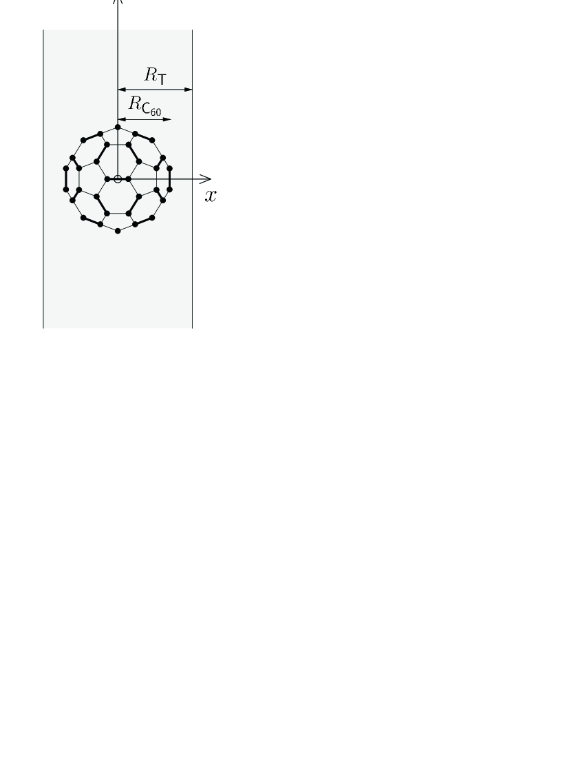
Figure 1: A single C${}_{\text{60}}$ molecule (radius $R_{\text{C${}_{\text{60}}$}}$) in a SWCNT (radius $R_{\text{T}}$). Shown is a projection onto the $(x,z)$-plane. The center of mass of the C${}_{\text{60}}$ molecule is chosen as the coordinate system’s origin. The tube’s long axis coincides with the $z$-axis; the C${}_{\text{60}}$ molecule is put in the standard orientation.

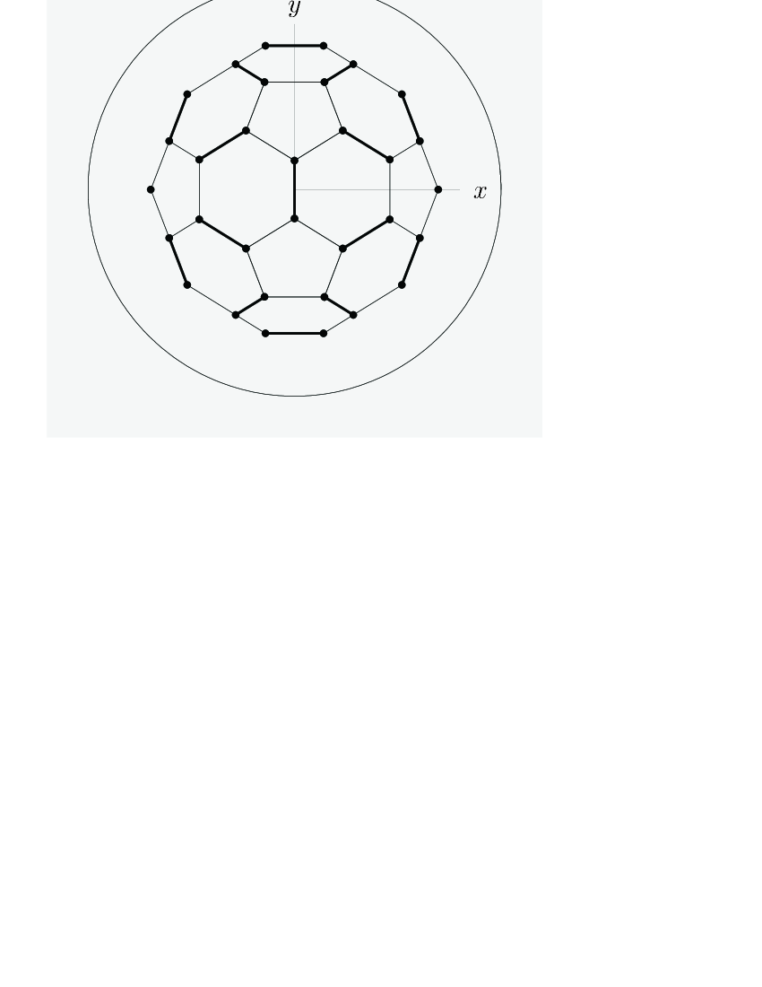
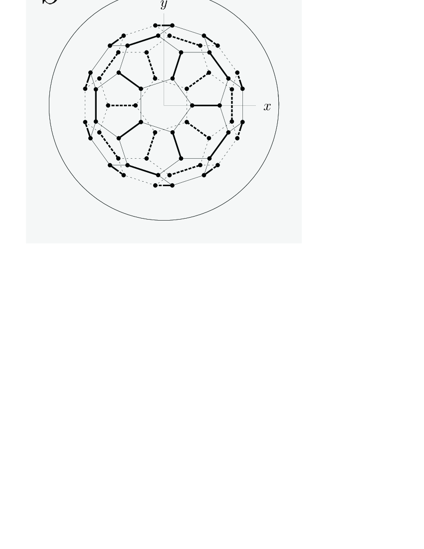
Figure 2: Special orientations of the C${}_{\text{60}}$ molecule: (a) standard orientation ($\alpha=\beta=\gamma=0$, double bonds perpendicular to the $z$-axis), (b) “pentagonal” orientation (pentagons perpendicular to the $z$-axis), (c) “hexagonal” orientations (hexagons perpendicular to the $z$-axis). Double bonds are drawn bolder than single bonds; dashed lines are located “beneath” the $(x,y)$-plane ($z\leq 0$). The surrounding tube is represented as a circular projection onto the $(x,y)$-plane. Note that a rotation about the $z$-axis over $-\alpha$ does not change double bonds, pentagons or hexagons — for Figs. (a), (b) and (c), respectively — being perpendicular to the $z$-axis.

For the description of the interaction between the C${}_{\text{60}}$ molecule and the nanotube we follow earlier work LamZeitschrift and treat the C${}_{\text{60}}$ molecule as a rigid cluster of interaction centers (ICs). Not only C atoms (‘a’) act as ICs, but also double bonds (‘db’) and single bonds (‘sb’). We label the 60 atoms by the index $\lambda_{\text{a}}=1,\ldots,60$. In the center of every of the 60 single bonds an IC is put, labelled by the index $\lambda_{\text{sb}}=1,\ldots,60$. On each of the 30 double bonds, 3 ICs dividing the bond in four equal parts are put, totalling to 90 db ICs, labelled $\lambda_{\text{db}}=1,\ldots,90$. Such a construction was originally introduced for modelling intermolecular interactions in solid C${}_{\text{60}}$ (C${}_{\text{60}}$ fullerite); having three ICs per double bond reflects the electronic density being smeared out along a double bond LamZeitschrift .

Every IC of the C${}_{\text{60}}$ molecule interacts with every atom of the nanotube via a pair interaction potential $v^{\text{t}}\bigl{(}|\vec{r}_{\tau}-\vec{r}_{\lambda_{\text{t}}}|\bigr{)}$, depending on the type of IC (‘t’ = ‘a’, ‘db’, ‘sb’). The total potential energy is then obtained by summing over all pair interactions:

$$V=\sum_{\tau}\sum_{\text{`t'}=\text{`a'},\text{`db'},\text{`sb'}}\sum_{\lambda_{\text{t}}}v^{\text{t}}\bigl{(}|\vec{r}_{\tau}-\vec{r}_{\lambda_{\text{t}}}|\bigr{)},$$ (2a)

where $$\tau \vec{r}_{\tau}$$ indexes the atoms of the tube and stands for their respective coordinates. As in Refs. MicVerNikPRL, and MicVerNikEPJB, , we use Born–Mayer–van der Waals pair interaction potentials:

$$v^{\text{t}}(r)=C_{1}^{t}e^{-C_{2}^{t}r}-\frac{B^{t}}{r^{6}}.$$ (2b)

Again, the use of such pair potentials was originally introduced for studying C$${}_{\text{60}} {}_{\text{60}} {}_{\text{60}} C_{1}^{t} C_{2}^{t} B^{t} \tau \vec{r}_{\tau}=(x_{\tau},y_{\tau},z_{\tau}) {}_{\text{60}}$$ - C interactions in C fullerite LamZeitschrift ; it lead to a crystal field potential and a structural phase transition temperature 124 ; 130 in good agreement with experiments. The potential constants , and used are those of Ref. MicVerNikEPJB, . In Eq. (2a), the sum over tube atoms, labelled by the index and having coordinates , can be restricted to atoms in a certain vicinity of the C molecule, realized by imposing the criterion

$$z_{\text{min}}\leq z_{\tau}\leq z_{\text{max}},$$ (2c)

with $z_{\text{min}}$ and $z_{\text{max}}$ cut-off values ensuring convergence.

In Refs. MicVerNikPRL and MicVerNikEPJB , a smooth-tube approximation to Eq. (2a) was presented. The actual network of carbon atoms making up the SWCNT is replaced by a homogeneous, cylindrical “carbonic” surface density with value $\sigma$ (units Å^-2). The C${}_{\text{60}}$ molecule-nanotube interaction energy is then rewritten as

$$V_{\text{smooth}}\\ =\sigma R_{\text{T}}\int_{0}^{2\pi}d\Phi\int_{-\infty}^{+\infty}dZ\sum_{\text{`t'}=\text{`a'},\text{`db'},\text{`sb'}}\sum_{\lambda_{\text{t}}}v^{\text{t}}\bigl{(}|\vec{\rho}-\vec{r}_{\lambda_{\text{t}}}|\bigr{)},$$ (3)

where $\vec{\rho}=(R_{\text{T}},\Phi,Z)$ is the cylindrical coordinate of a point on the tube ($x=R_{\text{T}}\cos\Phi$, $y=R_{\text{T}}\sin\Phi$, $z=Z$) and $R_{\text{T}}$ is the tube radius. The motivation for introducing approximation (3) is twofold. One reason is the dependence of $V_{\text{smooth}}$ on the tube radius $R_{\text{T}}$ rather than on the tube indices $(n,m)$. Indeed, $R_{\text{T}}$ remains the only relevant tube-characteristic parameter and as such simplifies a systematic investigation of carbon nanotubes. A further consequence of the tube’s cylindrical symmetry is the irrelevance of the Euler angle $\alpha$ (a final rotation of the C${}_{\text{60}}$ molecule over $-\alpha$ about the tube axis doesn’t matter) and of the $z$-coordinate $\zeta$ (for infinite or long-enough tubes). A second advantage of the smooth-tube ansatz is the possibility of performing an expansion of $V_{\text{smooth}}$ into symmetry-adapted rotator functions, a point we will return to in Sec. V. We stress the limited dependence of $V_{\text{smooth}}$ by writing

$$V_{\text{smooth}}\equiv V_{\text{smooth}}(\beta,\gamma;R_{\text{T}}).$$ (4)

To distinguish the smooth-tube approximation from the discrete case, we add the subscript ‘discrete’:

$$V\equiv V_{\text{discrete}}(\alpha,\beta,\gamma;\zeta;n,m),$$ (5)

where the actual expression is given by Eqs. (2a) – (2c).

In this paper we test the validity of smooth-tube approximation (3) by comparing $V_{\text{discrete}}$ and $V_{\text{smooth}}$ for a selection of tubes. Bearing in mind the three qualitatively different radii ranges ($R_{\text{T}}\lesssim 7$ Å, $7$ Å $\lesssim R_{\text{T}}\lesssim 7.9$ Å and $7.9$ Å $\lesssim R_{\text{T}}$) obtained in Ref. MicVerNikEPJB , we have selected zig-zag, armchair and chiral tubes with radii around $R_{\text{T}}=6.5$ Å, $R_{\text{T}}=7.5$ Å and $R_{\text{T}}=8.5$ Å. We have generated $(n,m)$ tubes starting from a graphene sheet with basis vectors $\vec{a}_{1}=a\vec{e}_{X}$ and $\vec{a}_{2}=a\frac{1}{2}\vec{e}_{X}+a\frac{3}{2}\vec{e}_{Y}$, where $\vec{e}_{X}$ and $\vec{e}_{Y}$ are planar cartesian basis vectors, and performing the roll-up along the vector $\vec{C}(n,m)=n\vec{a}_{1}+m\vec{a}_{2}$ Ham ; Saibook . The tube is then positioned so that the C atom originally (before rolling up) at $0\vec{e}_{X}+0\vec{e}_{Y}$ lies in the $(x,y)$ plane with $x$-coordinate $0$ and $y$-coordinate $R_{\text{T}}$ and that the cylinder containing the C atoms has its long axis coinciding with the $z$-axis. The C${}_{\text{60}}$ molecule is initially positioned so that its center of mass lies at the origin ($\zeta=0$); a translation along the $z$-axis away from the initial position is measured via the center of mass’ $z$-coordinate $\zeta$. The radius of the tube with indices $(n,m)$ reads $R_{\text{T}}=\frac{a}{2\pi}\sqrt{n^{2}+nm+m^{2}}$, with $a=2.49$ Å Ham ; Saibook ; the corresponding surface density has the value

$$\sigma=\frac{4}{\sqrt{3}a^{2}}=0.372\text{ {\AA}${}^{-2}$}.$$ (6)

A further tube parameter is its translational periodicity $\Delta z$, relevant when considering the $\zeta$-dependence of V${}_{\text{discrete}}$. While $\Delta z$ is small for non-chiral — i.e. zig-zag, $\Delta z=\sqrt{3}a$, and armchair, $\Delta z=a$ — tubes, the translational period can get very large for chiral tubes Saibook . A tube may also have an $s$-fold symmetry axis (coinciding with the $z$-axis) and therefore a rotational period $\Delta\alpha=2\pi/s$. When considering a tube with $s$-fold rotational symmetry it suffices to examine the interval $0\leq\alpha<\Delta\alpha$. The periodicities and other tube characteristics of our selected tubes are listed in Table 1.

Table 1: Characteristics of selected $(n,m)$ tubes. Tubes of all types (zig-zag, chiral and armchair) with radii $R_{\text{T}}$ as close to $6.5$ Å, $7.5$ Å and $8.5$ Å as possible were chosen. The angle $\Delta\alpha$ is the rotational period of the tube when performing a rotation about the $z$-axis. An expression for the calculation of the translational periodicity $\Delta z$ is given in Ref. Saibook, .

$(n,m)$	chirality	$R_{\text{T}}$ (Å)	$\Delta\alpha$	$\Delta z$ (Å)
$(16,0)$	zig-zag	$6.3407$	$2\pi/16$	$\sqrt{3}a=4.3128$
$(14,4)$	chiral	$6.4876$	$2\pi/2$	$35.3018$
$(9,9)$	armchair	$6.1176$	$2\pi/9$	$a=2.49$
$(19,0)$	zig-zag	$7.5296$	$2\pi/19$	$\sqrt{3}a$
$(16,5)$	chiral	$7.5296$	$2\pi$	$81.9433$
$(11,11)$	armchair	$7.5504$	$2\pi/11$	$a$
$(21,0)$	zig-zag	$8.3222$	$2\pi/21$	$\sqrt{3}a$
$(21,1)$	chiral	$8.5273$	$2\pi$	$92.8005$
$(12,12)$	armchair	$8.2369$	$2\pi/12$	$a$

III Mercator maps

To get a preliminary idea of how $V_{\text{smooth}}$ and $V_{\text{discrete}}$ compare, we have simply plot $V_{\text{smooth}}(\beta,\gamma,R_{\text{T}})$ and $V_{\text{discrete}}(\alpha=0,\beta,\gamma;\zeta=0;n,m)$ for each of the selected $(n,m)$ tubes in the form of Mercator maps Mercator . We stress that $(\alpha=0,\zeta=0)$ is but a particular case and that final conclusions should be made not only on the variation of $\beta$ and $\gamma$ but on the varying of $\alpha$ and $\zeta$ as well, as we will do later on. We do point out, however, that we expect the $\alpha$- and $\zeta$-dependencies to be of a lesser magnitude than the $\beta$- and $\gamma$-dependencies since the former correspond to a (final) rotation of the molecule about the $z$-axis (tube axis) over $-\alpha$ and a translation of the molecule along the $z$-axis, respectively, and hence relate to the tube structure rather than to the molecule structure. (As argued in the Introduction, a carbon nanotube can be regarded as being more “continuous” than a C${}_{\text{60}}$ molecule.)

As for the cut-off values, we have found — for $\zeta=0$ — that $z_{\text{min}}=-50$ Å and $z_{\text{max}}=50$ Å yield sufficient convergence. Note that the choice of $z_{\text{min}}$ and $z_{\text{max}}$ fixes the numbers $N_{\text{T}}$ of atoms to be taken into account in sum (2a). In principle, the tube fragment of length $L=z_{\text{max}}-z_{\text{min}}$ has a surface density $\tilde{\sigma}=N_{\text{T}}/(2\pi R_{\text{T}}L)$, differing from $\sigma$. We observe that differences between $\sigma$ and $\tilde{\sigma}$ are small, however. Although possibly (slightly) enhancing the agreement between $V_{\text{discrete}}$ and $V_{\text{smooth}}$, we have chosen not to calculate $V_{\text{smooth}}$ with $\tilde{\sigma}$ since it somehow relates to the tube structure — $N_{\text{T}}$ depends on $(n,m)$ — hence surpassing the smooth-tube approach’s underlying basic idea ($R_{\text{T}}$-dependence rather than $(n,m)$-dependence).

The Mercator maps $V_{\text{smooth}}(\beta,\gamma)\equiv V_{\text{smooth}}(\beta,\gamma;R_{\text{T}})$ and $V_{\text{discrete}}(\beta,\gamma)\equiv V_{\text{discrete}}(\alpha=0,\beta,\gamma;\zeta=0;n,m)$, respectively calculated via Eqs. (2a) – (2c) and (3) and both based on pair potential (2b), are shown as Figs. 3 – 5 for the tubes listed in Table 1. Figs. 3, 4 and 5 are for tubes with radii around $6.5$ Å, $7.5$ Å and $8.5$ Å, respectively. Within each figure, Subfigs. (a), (b) and (c) refer to zig-zag, chiral and armchair tubes; the left plot is $V_{\text{discrete}}$, the right $V_{\text{smooth}}$. Only the variation is plotted; for each plot the lowest occurring energy value, for which we write $V^{0}$, has been subtracted to make the minima lie at zero. The $V^{0}$ values for $V_{\text{discrete}}$ and $V_{\text{smooth}}$ and the the upper bounds of the left and right plots in Figs. 3 – 5 exhibit discrepancies. They originate from the intrinsic impossibility of the smooth-tube approximation to correctly account for the actual distribution of the carbon atoms on the cylinder. The wider the tube, the more atoms (the higher $N_{\text{T}}$), and the smaller the discrepancy: the $(9,9)$ tube ($V^{0}_{\text{smooth}}=70111.5$ K, $V^{0}_{\text{discrete}}=-79117.2$ K) exhibits the largest difference $V^{0}_{\text{discrete}}-V^{0}_{\text{smooth}}$ while for the $(21,1)$ tube the values $V^{0}_{\text{discrete}}$ and $V^{0}_{\text{smooth}}$ get very close ($V^{0}_{\text{smooth}}=-31028.6$ K, $V^{0}_{\text{discrete}}=-31033.9$ K). We point out that any continuum approach suffers from such a discrepancy, and that it can not be resolved by replacing $\sigma$ in Eq. (3) by the adjusted density $\tilde{\sigma}=N_{\text{T}}/(2\pi R_{\text{T}}2z_{\text{max}})$, a notion we illustrate in Appendix A. Nevertheless, it is not senseless at all to perform a smooth-tube approach, because conclusions are to be drawn based on the potential energy variation: of interest are the locations of energy minima, corresponding to molecular orientations which are most stable.

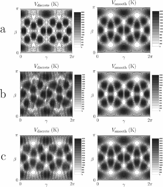
Figure 3: Mercator maps $V_{\text{discrete}}(\beta,\gamma)$ (left) and $V_{\text{smooth}}(\beta,\gamma)$ (right), units K: (a) $(n,m)=(16,0)$, (b) $(n,m)=(14,4)$, (c) $(n,m)=(9,9)$. The absolute minima values have been subtracted.

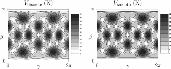
Figure 4: Mercator maps $V_{\text{discrete}}(\beta,\gamma)$ (left) and $V_{\text{smooth}}(\beta,\gamma)$ (right), units K, for the $(n,m)=(16,5)$ tube. The minimal values have been subtracted. The maps for the cases $(n,m)=(19,0)$ and $(11,11)$ look very similar to the $(16,5)$ maps.

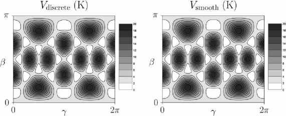
Figure 5: Mercator maps $V_{\text{discrete}}(\beta,\gamma)$ (left) and $V_{\text{smooth}}(\beta,\gamma)$ (right), units K, for the $(n,m)=(21,1)$ tube. The minimal values have been subtracted. The maps for the cases $(n,m)=(21,0)$ and $(12,12)$ are very similar to the $(21,1)$ maps.

The $V_{\text{smooth}}$ plots in Figs. 3(a), (b) and (c) are, apart from different energy ranges, similar. They exhibit 12 minima (white) and 20 maxima (dark gray). (The $\gamma$-coordinate, ranging from $0$ to $2\pi$, is cyclic, i.e. the molecular orientations at the $\gamma=0$ “edge” are repeated at the $\gamma=2\pi$ “edge”. The $\beta$-coordinate is not cyclic: points along the $\beta=0$ and $\beta=\pi$ “edges” with equal $\gamma$ refer to distinct configurations.) The 12 angle pairs $(\beta_{i},\gamma_{i})$ corresponding to minimal-energy configurations are tabulated in Table 2 and indicated schematically in Fig. 6. Each of the 12 minima corresponds to a molecular orientation where two opposing pentagons of the C${}_{\text{60}}$ molecule are perpendicular to the tube axis [Fig. 2(b)]; the Euler transformations $(\alpha=0,\beta_{i},\gamma_{i})$, $i=1,\ldots,12$, yield four truly different types of orientations (Fig. 7 and Table 2). The 20 maxima correspond to situations where two facing hexagons of the C${}_{\text{60}}$ molecule are perpendicular to the $z$-axis [Fig. 2(c)].

Table 2: Rotation angles $\beta_{i}$ and $\gamma_{i}$, $i=1,\ldots,12$, the corresponding Euler transformations ${\mathfrak{R}}^{-1}(\alpha=0,\beta_{i},\gamma_{i})$ of which make two facing pentagons of the C${}_{\text{60}}$ molecule lie perpendicular to the $z$-axis. For small tubes (see Fig. 3), the minima of $V_{\text{smooth}}(\beta,\gamma)$ occur at these 12 molecular orientations. Four distinct molecular orientations, labelled I, II, III and IV, are obtained, distinguishable by the orientation of the top ($z>0$) pentagon (Fig. 7).

$i$	$\beta_{i}$	$\gamma_{i}$	molecular orientation
$1$	$\beta_{0}=\cos^{-1}\frac{2}{\sqrt{10+2\sqrt{5}}}\approx 58^{\circ}$	$0$	I
$2$	$\pi-\beta_{0}$	$0$	II
$3$	$\frac{\pi}{2}$	$\beta_{0}$	III
$4$	$\frac{\pi}{2}-\beta_{0}$	$\frac{\pi}{2}$	II
$5$	$\frac{\pi}{2}+\beta_{0}$	$\frac{\pi}{2}$	I
$6$	$\frac{\pi}{2}$	$\pi-\beta_{0}$	IV
$7$	$\beta_{0}$	$\pi$	I
$8$	$\pi-\beta_{0}$	$\pi$	II
$9$	$\frac{\pi}{2}$	$\pi+\beta_{0}$	III
$10$	$\frac{\pi}{2}-\beta_{0}$	$\frac{3\pi}{2}$	II
$11$	$\frac{\pi}{2}+\beta_{0}$	$\frac{3\pi}{2}$	I
$12$	$\frac{\pi}{2}$	$2\pi-\beta_{0}$	IV

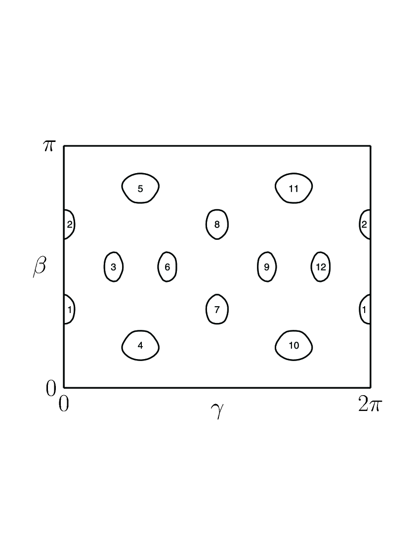
Figure 6: Indication of the locations $(\beta_{i},\gamma_{i})$, $i=1,\ldots,12$, tabulated in Table 2. For tubes with $R_{\text{T}}\approx 6.5$ Å (Fig. 3), these angle pairs correspond to the lowest-energy molecular orientations (Fig. 7). The contours are reproductions of the $V_{\text{smooth}}=200$ K contours of Fig. 3(a).

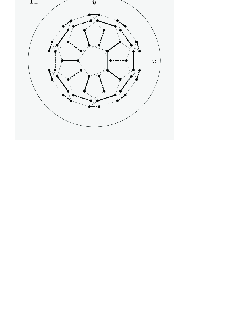
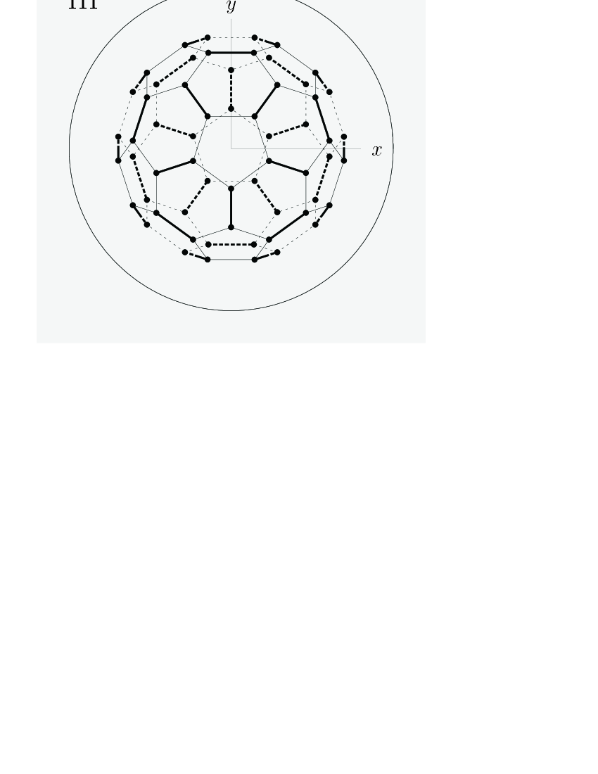
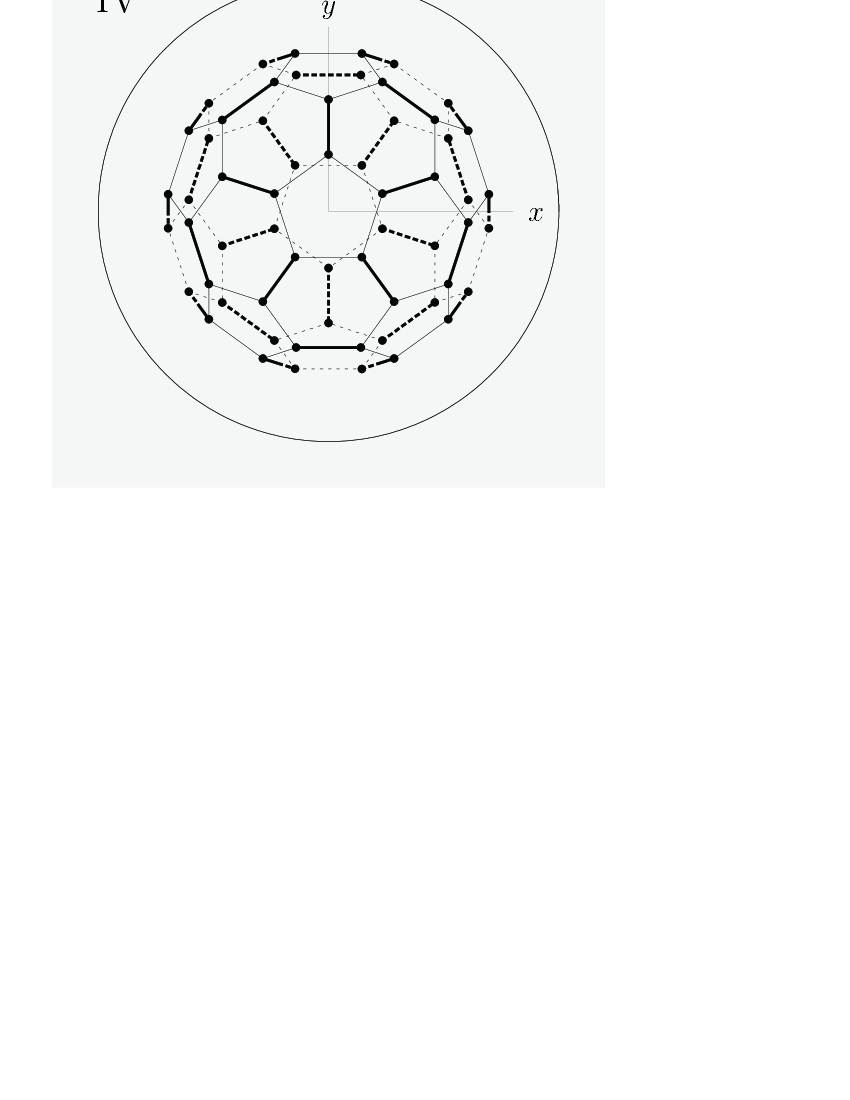
Figure 7: When applying the 12 Euler transformations ${\mathfrak{R}}^{-1}(\alpha=0,\beta_{i},\gamma_{i})$, with $(\beta_{i},\gamma_{i})$, $i=1,\ldots,12$, from Table 2, only four different molecular orientations the projections onto the $(x,y)$-plane of which are shown here, are obtained. Dashed (fragments of) lines have $z<0$. The labeling I, II, III and IV correlates with Table 2.

Comparing $V_{\text{discrete}}$ and $V_{\text{smooth}}$ of Fig. 3(a) — $(16,0)$ tube —, we see that the locations of minima and maxima hardly (or even do not) differ. For the $(9,9)$ armchair tube, Fig. 3(c), the energy ranges coincide, and the minima locations of $V_{\text{discrete}}$ and $V_{\text{smooth}}$ are, if not coinciding, almost equal. Deviations are observed in Fig. 3(b) for the chiral $(14,4)$ tube: the minima locations of $V_{\text{discrete}}$ clearly deviate somewhat from those of $V_{\text{smooth}}$; some even “split into two”. The deviations are small, however: one may write the true $V_{\text{discrete}}$ minima locations as $(\beta^{\prime}_{i}=\beta_{i}+\Delta\beta_{i},\gamma^{\prime}_{i}=\gamma_{i}+\Delta\gamma_{i})$. We estimate maximal deviation values at $|\Delta\beta_{i}|\approx 10^{\circ}$ and $|\Delta\gamma_{i}|\approx 12^{\circ}$.

For $R_{\text{T}}\approx 7.5$ Å (Fig. 4), the $V_{\text{discrete}}$ plots become extremely similar to the respective $V_{\text{smooth}}$ plots. For all three investigated tubes — $(19,0)$, $(16,5)$ and $(11,11)$ — the locations of minima (and maxima) can be concluded to coincide. The 30 minima correspond with two opposing double bonds being perpendicular to the tube axis [Fig. 2(a)]. Maximal energy occurs when two opposing pentagons are perpendicular to the tube axis (the 12 minimal-energy configurations for $R_{\text{T}}\approx 6.5$ Å, Fig. 3).

In Fig. 5, $R_{\text{T}}\approx 8.5$ Å, $V_{\text{discrete}}$ and $V_{\text{smooth}}$ match completely. With respect to Fig. 3, minima and maxima have been flipped: lowest-energy configurations now feature hexagons perpendicular to the tube axis, pentagons perpendicular to the tube axis yield the highest energy.

Up to now, $\alpha$ and $\zeta$ have been kept fixed. To get an idea of the energy variation when $\alpha$ and $\zeta$ are allowed to vary, we have calculated $V_{\text{discrete}}(\alpha,\beta=0,\gamma=0;\zeta=0;n,m)$ and $V_{\text{discrete}}(\alpha=0,\beta=0,\gamma=0;\zeta;n,m)$, for $0\leq\alpha\leq\Delta\alpha$ and $0\leq\zeta\leq\Delta\zeta$, respectively. The tube-dependent rotational and translational periods $\Delta\alpha$ and $\Delta\zeta$ are given in Table 1. In Table 3, we summarise these calculations by listing the differences $\Delta_{\alpha}V_{\text{discrete}}=\max\bigl{(}V_{\text{discrete}}(\alpha,\beta=0,\gamma=0;\zeta=0;n,m)\bigr{)}-\min\bigl{(}V_{\text{discrete}}(\alpha,\beta=0,\gamma=0;\zeta=0;n,m)\bigr{)}$ and $\Delta_{\zeta}V_{\text{discrete}}=\max\bigl{(}V_{\text{discrete}}(\alpha=0,\beta=0,\gamma=0;\zeta;n,m)\bigr{)}-\min\bigl{(}V_{\text{discrete}}(\alpha=0,\beta=0,\gamma=0;\zeta;n,m)\bigr{)}$ conveying the energy variation. Clearly, the tubes with $R_{\text{T}}\approx 6.5$ Å display fairly large energy fluctuations upon varying $\alpha$ and/or $\zeta$, as one might intuitively guess from the jagged contours in Fig. 3 (left). For intermediate ($R_{\text{T}}\approx 7.5$) and large tube radii ($R_{\text{T}}\approx 8.5$) the energy variations are small.

Table 3: Energy variations $\Delta_{\alpha}V_{\text{discrete}}$ and $\Delta_{\zeta}V_{\text{discrete}}$ (units K) when varying $\alpha$ or $\zeta$ and keeping other variables fixed.

$(n,m)$	$\Delta_{\alpha}V_{\text{discrete}}$ (K)	$\Delta_{\zeta}V_{\text{discrete}}$ (K)
$(16,0)$	$51.3$	$1079.3$
$(14,4)$	$643.2$	$639.6$
$(9,9)$	$665.9$	$8.3$
$(19,0)$	$<0.1$	$3.7$
$(16,5)$	$0.4$	$0.6$
$(11,11)$	$<0.1$	$<0.1$
$(21,0)$	$<0.1$	$0.1$
$(21,1)$	$<0.1$	$0.3$
$(12,12)$	$<0.1$	$<0.1$

We conclude that the smooth-tube approach works well for tube radii $R_{\text{T}}\approx 7.5$ Å and higher, as seen from the Mercator maps in Figs. 4 and 5 and the energy variations of Table 3. For small-radius tubes ($R_{\text{T}}\lesssim 7$ Å), a systematic investigation addressing the variation of $V_{\text{discrete}}$ as a function of $\alpha$, $\beta$, $\gamma$ and $\zeta$ is required. In the following section we perform such a study for the $(16,0)$, $(14,4)$ and $(9,9)$ and three more low-radius tubes.

IV Low-radius tubes: full energy variation

Before proceeding to the full energy variation calculation required for peapods with $R_{\text{T}}\approx 6.5$ Å, we would like to reflect on actual small values of peapod radii. To our knowledge, both today’s experimental and theoretical situation do not show unanimity. Theoretically, different lower limits for a peapod’s radius have been suggested, based on the outcome of the reaction energy $\Delta E$ in the reaction $(n,m)+\text{C${}_{\text{60}}$}\longrightarrow\text{C${}_{\text{60}}$@$(n,m)$}-\Delta E$: exo- ($\Delta E<0$) or endothermic ($\Delta E>0$). Okada et al. OkadaPRB2003 ; OkadaPRL2001 concluded from density-functional theory calculations that for C${}_{\text{60}}$@$(n,n)$ with $10\leq n\leq 13$ the reaction is exothermic, and, by extrapolating the results of $n=8,9$ and $10$, obtained a minimal tube radius of $R_{\text{T}}^{\text{min}}\approx 6.4$ Å OkadaPRL2001 . Rochefort Roc , performing molecular mechanics calculations, set the lower limit at $R_{\text{T}}^{\text{min}}\approx 5.9$ Å. From the experimental side, while it is still impossible to manufacture nanotubes — let alone peapods — with a given pair of indices $(n,m)$, peapod samples with a narrow radial dispersion around a mean value $\overline{R}_{\text{T}}$ and good filling rates (typically, $75\%$) can be produced at present. We mention a few (recent) experiments on peapods. Cambedouzou et al. Cam2005 used a sample with $\overline{R}_{\text{T}}\approx 6.8$ Å. Maniwa et al. Maniwa2003 fitted x-ray diffraction data on C${}_{\text{60}}$@SWCNT peapods to simulations, resulting in a mean radius $\overline{R}_{\text{T}}\approx 6.76$ Å. Kataura et al. KatauraAPA2002 reported measurements on a sample having a diameter range of $6.25$ Å $\leq R_{\text{T}}\leq 7.35$ Å, from which we calculate $\overline{R}_{\text{T}}\approx 6.8$ Å. The electron diffraction studies of Hirahara et al. Hir2001 were performed on peapod samples with $\overline{R}_{\text{T}}\approx 7.15$ Å (SWCNTs from a same batch were used to synthesize not only C${}_{\text{60}}$ -, but also C${}_{\text{70}}$ - and C${}_{\text{80}}$ peapods). Kataura et al. KatauraSynthMetals2001 reported high-yield fullerene encapsulation, controlling the tubes to be “larger than the $(10,10)$ tube”, i.e. $R_{\text{T}}^{\text{min}}\gtrsim 6.86$ Å. Pfeiffer et al. Pfe inferred from Raman spectroscopy their three samples to have $\overline{R}_{\text{T}}\approx 7$ Å, $\overline{R}_{\text{T}}\approx 6.52$ Å and $\overline{R}_{\text{T}}\approx 6.505$ Å. From all these values one may conclude that peapods with a radius around $6.5$ Å, our representative value for the “pentagonal case” (Figs. 3 and 7), although possible, are less abundant than peapods with a radius around, say, $6.75$ Å. We have therefore considered a few additional tubes — $(17,0)$, $(14,5)$ and $(10,10)$ — with radii around $6.75$ Å; their characteristics are shown in Table 4. These tubes can be expected to be more realistic representatives of the “pentagonal” regime instead of the $R_{\text{T}}=6.5$ Å tubes of Refs. MicVerNikPRL, and MicVerNikEPJB, — we recall that the transition from the “pentagonal” to the “double-bond” lowest-energy orientation occurs around $7$ Å MicVerNikEPJB . We note that the $(10,10)$ tube is of special interest since tubes with a radius close to $R_{\text{T}}(10,10)=6.86$ Å are favorable for C${}_{\text{60}}$ encapsulation, as seen in both experiment — according to Kataura et al. KatauraAPA2002 , peapod samples tend to have a radial dispersion centered around $R_{\text{T}}(10,10)$ — and theory — of the C${}_{\text{60}}$@$(n,n)$ series ($n=8,...,13$), the $n=10$ peapod stands out as the most “exothermic” (see above) OkadaPRB2003 ; OkadaPRL2001 .

Table 4: Characteristics of additional tubes ($R_{\text{T}}\approx 6.75$ Å). See captions to Tables 1 and 3.

$(n,m)$	chirality	$R_{\text{T}}$ (Å)	$\Delta\alpha$	$\Delta\zeta$ (Å)	$\Delta_{\alpha}V_{\text{discrete}}$ (K)	$\Delta_{\zeta}V_{\text{discrete}}$ (K)
$(17,0)$	zig-zag	$6.7370$	$2\pi/17$	$\sqrt{3}a=4.3128$	$<0.1$	$176.4$
$(14,5)$	chiral	$6.7603$	$2\pi$	$24.5237$	$36.3$	$36.5$
$(10,10)$	armchair	$6.8640$	$2\pi/10$	$a=2.49$	$23.1$	$11.6$

The Mercator maps $V_{\text{smooth}}(\beta,\gamma)$ and $V_{\text{discrete}}(\beta,\gamma)$ of the extra tubes are shown in Fig. 8; and the energy variations $\Delta_{\alpha}V_{\text{discrete}}$ and $\Delta_{\zeta}V_{\text{discrete}}$ are listed in Table 4. Again, minimal energies occur around $(\beta_{i},\gamma_{i})$, and maxima correspond to hexagons being perpendicular to the tube axis. The $(17,0)$ tube’s $V_{\text{discrete}}$ $50$ K contour deviates from its smooth-tube $50$ K contour [Fig. 8(a)], but there is some over-all agreement. The $(10,10)$ tube’s $V_{\text{discrete}}$ plot [Fig. 8(c), left] features “split” minima as seen for the $(14,4)$ tube [Fig. 3(b)]. The $(14,5)$ tube’s $V_{\text{discrete}}$ plot does not coincide nicely with its $V_{\text{smooth}}$ plot, but interestingly, the two locations $(\beta_{i},\gamma_{i})$, $i=3$ and $i=9$, type III “pentagonal” orientations, correspond very well to their smooth-approximation counterparts. Since all other ten minima locations are related to the $i=3$ or the $i=9$ location by a molecular rotation over $\alpha=\frac{\pi}{4}$ or $\alpha=\frac{\pi}{2}$ about the $z$-axis — see Fig. 7 —, any of the $(\beta_{i},\gamma_{i})$ points can be made a minimal configuration by changing $\alpha$. The main conclusion is that the minimal-energy orientation will always feature facing pentagons perpendicular to the $z$-axis. The same can be said of any of the tubes of Figs. 3 and 8 — tubes with $R_{\text{T}}\lesssim 7$ Å — excepting the $(14,4)$ tube.

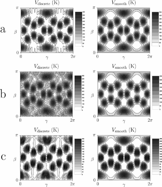
Figure 8: Mercator maps $V_{\text{discrete}}(\beta,\gamma)$ (left) and $V_{\text{smooth}}(\beta,\gamma)$ (right), units K: (a) $(n,m)=(17,0)$, (b) $(n,m)=(14,5)$, (c) $(n,m)=(10,10)$. The minimal values have been subtracted.

We now turn to the $\alpha$- and $\zeta$-dependencies of $V_{\text{discrete}}$. It is sufficient to consider the intervals $0\leq\alpha<\Delta\alpha\equiv\alpha_{\text{max}}$ and $0\leq\zeta<\Delta\zeta\equiv\zeta_{\text{max}}$. We divide the interval $[0,\alpha_{\text{max}}[\times[0,\zeta_{\text{max}}[$ into a $10\times 10$ grid $(\alpha_{i=1,\ldots,10},\zeta_{j=1,\ldots,10})$, $\alpha_{i}=(i-1)\frac{\alpha_{\text{max}}}{10}$, $\zeta_{j}=(j-1)\frac{\zeta_{\text{max}}}{10}$, and construct a double Fourier series — for notational simplicity we drop the indices $(n,m)$ —,

$$V_{\text{discrete}}(\alpha,\beta,\gamma;\zeta)\\ =\sum_{p=0}^{\infty}\sum_{q=0}^{\infty}\Biggl{\{}A_{pq}(\beta,\gamma)\cos\biggl{(}p\frac{\alpha}{\alpha_{\text{max}}}2\pi\biggr{)}\cos\biggl{(}q\frac{\zeta}{\zeta_{\text{max}}}2\pi\biggr{)}\\ +B_{pq}(\beta,\gamma)\sin\biggl{(}p\frac{\alpha}{\alpha_{\text{max}}}2\pi\biggr{)}\cos\biggl{(}q\frac{\zeta}{\zeta_{\text{max}}}2\pi\biggr{)}\\ +C_{pq}(\beta,\gamma)\cos\biggl{(}p\frac{\alpha}{\alpha_{\text{max}}}2\pi\biggr{)}\sin\biggl{(}q\frac{\zeta}{\zeta_{\text{max}}}2\pi\biggr{)}\\ +D_{pq}(\beta,\gamma)\sin\biggl{(}p\frac{\alpha}{\alpha_{\text{max}}}2\pi\biggr{)}\sin\biggl{(}q\frac{\zeta}{\zeta_{\text{max}}}2\pi\biggr{)}\Biggr{\}},$$ (7)

by numerically calculating the Fourier coefficients

$$A_{pq}(\beta,\gamma)\\ =N_{pq}\int_{0}^{\alpha_{\text{max}}}d\alpha\,\int_{0}^{\zeta_{\text{max}}}d\zeta\,V_{\text{discrete}}(\alpha,\beta,\gamma;\zeta)\\ \times\cos\biggl{(}p\frac{\alpha}{\alpha_{\text{max}}}2\pi\biggr{)}\cos\biggl{(}q\frac{\zeta}{\zeta_{\text{max}}}2\pi\biggr{)},\\ \ldots$$ (8)

via the trapezium-rule approximations

$$A_{pq}(\beta,\gamma)\\ \approx N_{pq}\sum_{i=1}^{10}\sum_{j=1}^{10}\frac{\alpha_{\text{max}}}{10}\frac{\zeta_{\text{max}}}{10}V_{\text{discrete}}(\alpha_{i},\beta,\gamma;\zeta_{j})\\ \times\cos\biggl{(}p\frac{\alpha_{i}}{\alpha_{\text{max}}}2\pi\biggr{)}\cos\biggl{(}q\frac{\zeta_{j}}{\zeta_{\text{max}}}2\pi\biggr{)},\\ \ldots$$ (9)

The coefficients $B_{pq}$, $C_{pq}$ and $D_{pq}$ are obtained by replacing $\cos()\cos()$ by $\sin()\cos()$, $\cos()\sin()$ and $\sin()\sin()$, respectively. The prefactors read

$$N_{00} =\frac{1}{\alpha_{\text{max}}\zeta_{\text{max}}},$$

$$N_{0s} =N_{r0}=\frac{2}{\alpha_{\text{max}}\zeta_{\text{max}}},$$

$$N_{rs} =\frac{4}{\alpha_{\text{max}}\zeta_{\text{max}}},$$ (10)

where $r$ and $s\neq 0$. In series (7), some terms may vanish because of symmetry reasons.

The Fourier coefficients $A_{pq}(\beta,\gamma)$, $B_{pq}(\beta,\gamma)$, $C_{pq}(\beta,\gamma)$, $D_{pq}(\beta,\gamma)$ can be interpreted as Mercator maps. The magnitude of the coefficients decreases for increasing indices $p$ and $q$; we approximate $V_{\text{discrete}}(\alpha,\beta,\gamma;\zeta)$ by

$$\tilde{V}_{\text{discrete}}(\alpha,\beta,\gamma;\zeta)=\sum_{p=0}^{4}\sum_{q=0}^{4}\Biggl{\{}A_{pq}(\beta,\gamma)\\ \times\cos\biggl{(}p\frac{\alpha}{\alpha_{\text{max}}}2\pi\biggr{)}\cos\biggl{(}q\frac{\zeta}{\zeta_{\text{max}}}2\pi\biggr{)}+\ldots\Biggr{\}}.$$ (11)

For given $\beta$ and $\gamma$, we scan the $\alpha$- and $\zeta$-intervals and define

$$\tilde{V}_{\text{discrete}}^{\text{min}}(\beta,\gamma)\equiv\min\bigl{\{}\tilde{V}_{\text{discrete}}(\alpha,\beta,\gamma;\zeta);\\ 0\leq\alpha\leq\alpha_{\text{max}}0\leq\zeta\leq\zeta_{\text{max}}\bigr{\}}.$$ (12)

The quantity $\tilde{V}_{\text{discrete}}^{\text{min}}(\beta,\gamma)$, gives the lowest attainable energy $\tilde{V}_{\text{discrete}}$ when varying $\alpha$ and $\zeta$. In Fig. 9, it has been plotted for every of the six tubes investigated. The plots again exhibit icosahedral symmetry as in the previous Mercator maps. The main observation here is that for all tubes, except the $(9,9)$ tube [Fig. 9(c), left], the absolute minima lie not precisely at the 12 $(\beta_{i},\gamma_{i})$ locations but somewhat away from them — the same effect observed for the $(\alpha=0,\zeta=0)$ V${}_{\text{discrete}}$ plots in Figs. 3 and 8. As before, we can write the actual minimum locations as $(\beta^{\prime}_{i}=\beta_{i}+\Delta\beta_{i},\gamma^{\prime}_{i}=\gamma_{i}+\Delta\gamma_{i})$. For the $R_{\text{T}}\approx 6.5$ Å tubes (Fig. 9, left), excepting the $(9,9)$ tube, the $(\beta_{i},\gamma_{i})$ locations (orientations) have energies $\sim 300$ K higher than the minimal energies. The $(9,9)$ tube’s minima are really close to — if not, coinciding with — the $(\beta_{i},\gamma_{i})$ orientations. For the $R_{\text{T}}\approx 6.75$ Å tubes (Fig. 9, right), excepting the $(10,10)$ tube, the $(\beta_{i},\gamma_{i})$ orientations have energies $\sim 20$ K higher than the minimal energies. The $(10,10)$ tube’s absolute minima lie also off the $(\beta_{i},\gamma_{i})$ “pentagon” orientations (not visible on the plot), and have energies $\sim 12$ K higher than the lowest energies. We must therefore conclude that chirality-dependent effects manifest themselves here. However, for $R_{\text{T}}\approx 6.75$ Å tubes, probably the smallest peapod tubes as discussed above, the effects can be said to be minor. As an approximation, one may consider the smooth-tube approach. We recall that for higher tube radii, the smooth-tube approximation is excellent (when the C${}_{\text{60}}$ molecules lie on the tube axis).

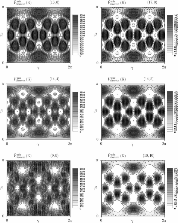
Figure 9: Mercator maps $\tilde{V}_{\text{discrete}}(\beta,\gamma)$, units K, for $(16,0)$, $(14,4)$, $(9,9)$, $(17,0)$, $(14,5)$ and $(10,10)$ peapods. The minimal values have been subtracted.

To conclude this section, we come back to the 4 types of “pentagonal” orientations depicted in Fig. 7. We recall that they arise from the Euler transformations $\mathfrak{R}^{-1}(\alpha=0,\beta_{i},\gamma_{i})$ with the angle pairs $(\beta_{i},\gamma_{i})$, $i=1,\ldots,12$, of Table 2. Clearly, all 12 $V_{\text{smooth}}(\beta_{i},\gamma_{i})$ values are identical because of the cylindrical symmetry. A priori, $V_{\text{discrete}}(\beta_{i},\gamma_{i})$ can be different for each of the four types I, II, III and IV. Interestingly, depending on the tube’s symmetry, some orientations sometimes are equivalent. This is illustrated in Table 5, and can be understood by being aware of certain symmetry elements. Orientations I and II are related via a rotation over $\pi$ about the $z$-axis, and likewise for orientations III and IV. Orientations III and I are related by a rotation over $\pi/2$ about the $z$-axis. The presence of a twofold symmetry axis for the $(n,m)$ tube therefore implies equivalence of orientations I and II and of orientations III and IV, while a fourfold axis implies the equivalence of all orientations. The $(16,0)$ tube is an example of the latter, a $(14,4)$ tube provides an example of the former. The $(16,5)$ tube has no pure rotational symmetry axis and exhibits therefore distinguishable $V_{\text{discrete}}$ values. We note that any occurring energy differences as a result of the discussed inequivalences are small, however, and not seen on any of the Mercator maps since the contour values lie not sufficiently close to each other. Also note that these observations are generally true for the values $V_{\text{discrete}}(\beta_{i},\gamma_{i})$ — they do not need to be to minima, e.g. the $(14,4)$ tube [Fig. 3(b)]. The equivalence relationships between the twelve $(\beta_{i},\gamma_{i})$ orientations is nicely seen in the the $(14,5)$ tube’s $V_{\text{discrete}}$ plot [Fig. 8(b)]: all 4 types I ($\left\{1,5,7,11\right\}$), II ($\left\{2,4,8,10\right\}$), III ($\left\{3,9\right\}$) and IV ($\left\{6,12\right\}$) “behave” differently. When making the observations concerning the equality/inequality of $V_{\text{smooth}}(\beta_{i},\gamma_{i})$ values summarized schematically in Table 5, we have made sure that sufficient numerical accuracy has been achieved. One needs accurate enough atomic coordinates of the C${}_{\text{60}}$ molecule, so that upon explicitly applying coordinate transforms ${\mathfrak{R}}^{-1}(\alpha,\beta,\gamma)$ corresponding to symmetry elements of the C${}_{\text{60}}$ molecule (i.e., of the icosahedral group $I_{h}$), the same set of coordinates is obtained up to the desired accuracy. We use coordinates with 12 significant digits.

Table 5: Schematical presentation of $V_{\text{discrete}}(\beta_{i},\gamma_{i})$ values for selected tubes, indicating equalities and inequalities due to the presence/absence of certain symmetries. The angles $\beta_{i}$ and $\gamma_{i}$ are tabulated in Table 7, the corresponding molecular orientations depicted in Fig. 2.

$i$ (type)	$V_{\text{discrete}}(\beta_{i},\gamma_{i})$
	$(n,m)=(16,0)$	$(n,m)=(14,4)$	$(n,m)=(16,5)$
$1,5,7,11$ (I)	$V^{(16,0)}_{1}$	$V^{(14,4)}_{1}$	$V^{(16,5)}_{1}$
$2,4,8,10$ (II)	$V^{(16,0)}_{1}$	$V^{(14,4)}_{1}$	$V^{(16,5)}_{2}$
$3,9$ (III)	$V^{(16,0)}_{1}$	$V^{(14,4)}_{3}$	$V^{(16,5)}_{3}$
$6,12$ (IV)	$V^{(16,0)}_{1}$	$V^{(14,4)}_{3}$	$V^{(16,5)}_{6}$

V Discussion and conclusions

We have presented a systematic comparison of the potential energy of a C${}_{\text{60}}$ molecule — treated as an icosahedral cluster of ICs — encapsulated centrally in a SWCNT, when approximating the tube as a uniform cylinder and when taking the true carbon atomic network into account. The former approach results in only two variables (the Euler angles $\beta$ and $\gamma$), while the latter requires in addition a third Euler angle $\alpha$ and the molecule’s $z$-coordinate $\zeta$ denoting its position along the tube axis. The $(\beta,\gamma)$-dependence can be conveniently plot as a Mercator map. Fixing $(\alpha,\zeta)$ at $(0,0)$ then allows a first visual comparison of the “smooth” and “discrete” Mercator maps $V_{\text{smooth}}(\beta,\gamma)$ and $V_{\text{discrete}}(\beta,\gamma)$. From these preliminary comparisons one can see that the larger the tube, the better the smooth-tube approximation. Indeed, the $V_{\text{smooth}}$ and $V_{\text{discrete}}$ Mercator maps for tubes with radii $R_{\text{T}}\gtrsim 7.5$ Å (Figs. 4 and Fig. 5) are as good as identical. For smaller tubes, the effect of the tube structure comes into play and deviations between the smooth and discrete Mercator maps are visible (Figs. 3 and Fig. 8). While the $(\alpha,\zeta)$-dependence of $V_{\text{discrete}}$ can be argued to be negligible for the larger tubes ($R_{\text{T}}\gtrsim 7$ Å) because of the similarity of $V_{\text{smooth}}(\beta,\gamma)$ and $V_{\text{discrete}}(\beta,\gamma)$, a full investigation of the variables $\alpha$ and $\zeta$ is in order for smaller tubes. We have presented a detailed study for selected zig-zag, chiral and armchair tubes with radii around $R_{\text{T}}\approx 6.5$ Å and $6.75$ Å, including the $(10,10)$ tube, nowadays considered the ideal peapod tube KatauraAPA2002 ; OkadaPRB2003 ; OkadaPRL2001 .

A double Fourier series captures the $(\alpha,\zeta)$-dependence in a manageable way. Scanning $V_{\text{discrete}}(\alpha,\beta,\gamma;\zeta;n,m)$ for its lowest attainable values when varying $\alpha$ and $\zeta$ yields Mercator maps similar to $V_{\text{smooth}}(\beta,\gamma;n,m)$. We see that the actual energy minima do not correspond to the 12 “pentagonal” $(\beta_{i},\gamma_{i})$ orientations but that they lie slightly away from them (except for the $(9,9)$ tube, where the minimal-energy molecular configurations are really close to the “pentagonal” orientations). Such $(\beta,\gamma)$ orientations correspond to “tilted” molecules, where an axis connecting the midpoints of two opposing pentagons does not coincide with the tube’s long axis ($z$-axis) but makes a cone with a small opening angle if one would perform the $\alpha$ Euler rotation. Hence, we conclude that for these smaller tubes (again excepting the $(9,9)$ tube), the chirality of the tube does play a role. However, as seen from the small deviations occurring in the Mercator plots, the effect is not strong, especially for the $R_{\text{T}}\approx 6.75$ Å tubes (Fig. 9, right). Therefore, one may consider the smooth-tube approach if one wants to capture radius-dependent properties. In this respect, one should be aware of the present-day experimental situation: precise knowledge of the components (i.e., occurring chiralities) in a peapod sample is absent — only a determination of the tube radius distribution seems feasible up to now. The main conclusion of Refs. MicVerNikPRL, and MicVerNikEPJB stands: three regimes can be distinguished ($R_{\text{T}}\lesssim 7$ Å, “pentagonal” orientation, $7$ Å $\lesssim R_{\text{T}}\lesssim 7.9$ Å, “double-bond” orientation and $R_{\text{T}}\gtrsim 7.9$ Å, “hexagonal” orientation). The “pentagonal” orientations have to be restated as “tilted pentagonal” orientations, though. Generally, our findings are in accordance with those of Troche et al. Troche who concluded that the chirality of the SWCNT encapsulating the C${}_{\text{60}}$ molecules has only a minor effect.

Note that transversal motion of the C${}_{\text{60}}$ molecule (off-axis displacements) is not discussed here since our sole purpose was a direct comparison of the smooth-tube and the discrete-tube approaches for a centrally located C${}_{\text{60}}$ molecule. As expected intuitively and demonstrated in Refs. MicVerNikPRL, and MicVerNikEPJB, , from a certain radius ($R_{\text{T}}\approx 7$ Å) on, an off-center position is energetically more favorable. This, however, involves energy differences much larger than those seen upon varying $\beta$, $\gamma$, $\alpha$ and $\zeta$.

The smooth-tube approximation’s requiring only the two Euler angles $\beta$ and $\gamma$ allows for the use of symmetry-adapted rotator functions. For details we refer to Refs. MicVerNikPRL, and MicVerNikEPJB, . The advantage lies in the possibility of writing $V_{\text{smooth}}(\beta,\gamma;R_{\text{T}})$ as an expansion into functions ${\mathfrak{U}}_{l}(\beta,\gamma)$ taking the icosahedral molecular symmetry of the C${}_{\text{60}}$ molecule and the cylindrical symmetry of its site into account,

$$V_{\text{smooth}}(\beta,\gamma;R_{\text{T}})=\sum_{l=0}^{\infty}w_{l}(R_{\text{T}}){\mathfrak{U}}_{l}(\beta,\gamma),$$ (13)

where the coefficients $w_{l}$ relate to the icosahedral symmetry and carry the details of the pair interaction potential. The molecular symmetry implies the first non-vanishing terms to be those with $l=0$, $l=6$, $l=10$ and $l=12$, and a restriction to only these four leading terms already approximates $V_{\text{smooth}}(\beta,\gamma;R_{\text{T}})$ extremely well. Apart from providing mathematical/physical clarity, expansion (13) greatly reduces the calculation time. While, for a $100\times 100$ $(\beta,\gamma)$ grid, an implementation of Eq. (3) takes hours, the calculation of $V_{\text{smooth}}(\beta,\gamma;R_{\text{T}})$ via Eq. (13) is a matter of minutes on the same machine.

It is interesting to note that double-walled carbon nanotubes (DWCNTs) allow the encapsulation of C${}_{\text{60}}$ molecules in inner spaces smaller than observed for SWCNTs: Khlobystov et al. Khl reported the insertion of C${}_{\text{60}}$ molecules in DWCNTs with internal radii as small as $5.5$ Å. Having different minimal internal radii of SWCNTs and DWCNTs for filling with C${}_{\text{60}}$ molecules is attributed to the difference in how a C${}_{\text{60}}$ molecule interacts with a SWCNT and a DWCNT Khl . We have carried out calculations for C${}_{\text{60}}$@DWCNT by treating the field on the C${}_{\text{60}}$ molecule as a superposition of the two fields from the tubes with different radii. Although we find that the presence of a second (outer) tube decreases the energy for encapsulation when taking a tube radius difference equalling the interlayer distance of graphite ($3.35$ Å), the effect is rather small and not sufficient to explain the large reduction in inner tube radius.

We believe that the general conclusion — the smooth-tube approximation being justified for intermediate and large tube radii ($R_{\text{T}}\gtrsim 7$ Å) and possibly acceptable for smaller tube-radii — reached here is relevant for other peapod systems. For example, (C${}_{\text{70}}$)_N@SWCNT peapods feature different orientations of the encapsulated C${}_{\text{70}}$ molecules for different tube radii Maniwa2003 ; Hir2001 , the so-called “lying” (for smaller tube radii) and “standing” (larger tube radii) orientations. A smooth-tube approach would make a good start for investigating these specific orientations.

Appendix A Discrepancy test

We consider a single carbon atom in a short $(16,0)$ tube fragment defined by $|z_{\tau}|\leq a/\sqrt{3}\approx 1.42$ Å, leaving only three “rings” of $16$ carbon atoms each. The tube atoms have coordinates $\vec{r}_{\tau}=(x_{\tau},y_{\tau},z_{\tau})$, $\tau=1,\ldots,48$. The single atom, put at the center of the fragment which we define to be the origin of the employed cartesian coordinates system, has a “discrete” energy

$$V_{\text{discrete}}=\sum_{\tau=1}^{48}v^{\text{a}}(r_{\tau}),$$ (14)

approximated by the “smooth” energy

$$V_{\text{smooth}}=\sigma R_{\text{T}}\int_{0}^{2\pi}d\Phi\int_{Z_{\text{min}}}^{Z_{\text{max}}}dZv^{\text{a}}(\vec{\rho}).$$ (15)

In both equations, the pair potential $v^{\text{a}}(r)$ of Sec. II is understood. In Eq. (15), $\Phi$ and $Z$ are defined via $x=R_{\text{T}}\cos\Phi$, $y=R_{\text{T}}\sin\Phi$ and $z=Z$. The integration boundaries $Z_{\text{min}}$ and $Z_{\text{max}}$ are not well-defined. Indeed, there is a range of both lower and upper boundaries corresponding to a “smooth” tube fragment containing only the three “rings” with $z_{\tau}=-a/\sqrt{3}$, $z_{\tau}=0$ and $z_{\tau}=a/(2\sqrt{3})$: $-\sqrt{3}a/2<Z_{\text{min}}\leq-a/\sqrt{3}$ and $a/(2\sqrt{3})\leq Z_{\text{max}}<\sqrt{3}a/2$. In Table 6 we present $V_{\text{smooth}}$ values calculated for a few of these $[Z_{\text{min}},Z_{\text{max}}]$ intervals. For each case, both the tube surface density $\sigma=4/(\sqrt{3}a^{2})$ and the adjusted tube density $\tilde{\sigma}=48/\bigl{(}2\pi R_{\text{T}}(Z_{\text{max}}-Z_{\text{min}})\bigr{)}$ has been considered. The “discrete” value, obtained via Eq. (14), reads $V_{\text{discrete}}=-318.1$ K, and is best reproduced by the “smooth” value if the interval $[Z_{\text{min}},Z_{\text{max}}]=[-\frac{5a}{4\sqrt{3}},\frac{a}{\sqrt{3}}]$ is chosen. The tube fragment edges then lie precisely in the middle of two neighboring “rings” of atoms; the surface densities $\sigma$ and $\tilde{\sigma}$ then happen to coincide. The values of table 6 suggest that some choice(s) of intervals may yield the $V_{\text{discrete}}$ value, but the point we want to make here is that making use of the adjusted surface density $\tilde{\sigma}$ does not “convert” the $V_{\text{smooth}}$ to the $V_{\text{discrete}}$ value. We remark that doing the $V_{\text{smooth}}$ calculations described in the paper with $\tilde{\sigma}$ instead of $\sigma$ turned out to yield only very small differences.

Table 6: $V_{\text{smooth}}$ values, units K, for various tube fragments and surface densities $\sigma$ and $\tilde{\sigma}$.

$[Z_{\text{min}},Z_{\text{max}}]$	$\sigma$ or $\tilde{\sigma}$	$V_{\text{smooth}}$ (K)
$[-\frac{\sqrt{3}a}{2},\frac{\sqrt{3}a}{2}]$	$\sigma$	$-405.0$
$[-\frac{\sqrt{3}a}{2},\frac{\sqrt{3}a}{2}]$	$\tilde{\sigma}$	$-303.7$
$[-\frac{5a}{4\sqrt{3}},\frac{a}{\sqrt{3}}]$	$\sigma$	$-317.0$
$[-\frac{5a}{4\sqrt{3}},\frac{a}{\sqrt{3}}]$	$\tilde{\sigma}$	$-317.0$
$[-\frac{a}{\sqrt{3}},\frac{a}{2\sqrt{3}}]$	$\sigma$	$-217.1$
$[-\frac{a}{\sqrt{3}},\frac{a}{2\sqrt{3}}]$	$\tilde{\sigma}$	$-325.7$

References

- (1) S. Iijima, Nature (London) 354, 56 (1991).
- (2) T.W. Ebbesen and P.M. Ajayan, Nature (London) 358, 220 (1992).
- (3) R. Saito, G. Dresselhaus, and M.S. Dresselhaus, Physical Properties of Carbon Nanotubes (Imperial College Press, London, 1998).
- (4) P.J.F. Harris, Carbon Nanotubes and Related Structures (Cambridge University Press, Cambridge, 1999).
- (5) J. Sloan, A.I. Kirkland, J.L. Hutchison and M.L.H. Green, Chem. Commun., 1319 (2002).
- (6) M. Monthioux, Carbon 40, 1809 (2002).
- (7) B.W. Smith, M. Monthioux, and D.E. Luzzi, Nature (London) 396, 323 (1998).
- (8) D.J. Hornbaker, S.J. Kahng, S. Misra, B.W. Smith, A.T. Johnson, E.J. Mele, D.E. Luzzi, and A. Yazdani, Science 295, 829 (2002).
- (9) B.W. Smith, M. Monthioux, and D.E. Luzzi, Chem. Phys. Lett. 315, 31 (1999).
- (10) B. Burteaux, A. Claye, B.W. Smith, M. Monthioux, D.E. Luzzi, and J.E. Fischer, Chem. Phys. Lett. 310, 21 (1999).
- (11) G.T. Pickett, M. Gross, and H. Okuyama, Phys. Rev. Lett. 85, 3652 (2000).
- (12) M. Hodak and L.A. Girifalco, Phys. Rev. B 67, 075419 (2003).
- (13) A. Khlobystov, D.A. Britz, A. Ardavan, and G.A.D. Briggs, Phys. Rev. Lett. 92, 245507 (2004).
- (14) K.S. Troche, V.R. Coluci, S.F. Braga, D.D. Chinellato, F. Sato, S.B. Legoas, R. Rurali, and D.S. Galvao, Nano Lett. 5, 349 (2005).
- (15) K.H. Michel, B. Verberck, and A.V. Nikolaev, Phys. Rev. Lett. 95, 185506 (2005).
- (16) K.H. Michel, B. Verberck, and A.V. Nikolaev, Eur. Phys. J. B 48, 113 (2005).
- (17) W. Mickelson, S. Aloni, W.Q. Han, J. Cummings, and A. Zettl, Science 300, 467 (2003).
- (18) C.J. Bradley and A.P. Cracknell, The Mathematical Theory of Symmetry in Solids (Clarendon, Oxford, 1972).
- (19) W.I.F. David, R.M. Ibberson, J.C. Matthewman, K. Prassides, T.J.S. Dennis, J.P. Hare, H.W. Kroto, R. Taylor, and D.R.M. Walton, Nature (London) 353, 147 (1991).
- (20) D. Lamoen and K.H. Michel, Z. Phys. B 92, 323 (1993); J.R.D. Copley and K.H. Michel, J. Phys.: Condens. Matter 5, 4353 (1993).
- (21) P. Launois, S. Ravy, and R. Moret, Phys. Rev. B 55, 2651 (1997).
- (22) K.H. Michel and J.R.D. Copley, Z. Phys. B 103, 369 (1997).
- (23) N. Hamada, S. Sawada, and A. Oshiyama, Phys. Rev. Lett. 68, 1579 (1992); D.H. Robertson, D.W. Brenner, and J.W. Mintmire, Phys. Rev. B 45, 12592 (1992).
- (24) Gerardus Mercator (1512 - 1594), Flemish cartographer, inventor of the cylindrical projection. The angles and play the role of geographical lattitude and longitude, respectively.
- (25) S. Okada, M. Otani, and A. Oshiyama, Phys. Rev. B 67, 205411 (2003).
- (26) S. Okada, S. Saito, and A. Oshiyama, Phys. Rev. Lett. 86, 3835 (2001).
- (27) A. Rochefort, Phys. Rev. B 67, 115401 (2003).
- (28) J. Cambedouzou, V. Pichot, S. Rols, P. Launois, P. Petit, R. Klement, H. Kataura, and R. Almairac, Eur. Phys. J. B 42, 31 (2004); J. Cambedouzou, S. Rols, R. Almairac, J.-L. Sauvajol, H. Kataura, and H. Schober, Phys. Rev. B 71, 041403(R) (2005).
- (29) Y. Maniwa, H. Kataura, M. Abe, A. Fujiwara, R. Fujiwara, H. Kira, H. Tou, S. Suzuki, Y. Achiba, E. Nishibori, M. Takata, M. Sakata, and H. Suematsu, J. Phys. Soc. Jap. 72, 45 (2003).
- (30) H. Kataura, Y. Maniwa, M. Abe, A. Fujiwara, T. Kodama, K. Kikuchi, H. Imahori, Y. Misaki, S. Suzuki, and Y. Achiba, Appl. Phys. A: Mater. Sci. Process. 74, 349 (2002).
- (31) K. Hirahara, S. Bandow, K. Suenaga, H. Kato, T. Okazaki, H. Shinohara, and S. Iijima, Phys. Rev. B 64, 115420 (2001).
- (32) H. Kataura, Y. Maniwa, T. Kodama, K. Kikuchi, K. Hirahara, K. Suenaga, S. Iijima, S. Susuki, Y. Achiba, and W. Krätschmer, Synth. Met. 121, 1195 (2001).
- (33) R. Pfeiffer, H. Kuzmany, T. Pichler, H. Kataura, Y. Achiba, M. Melle-Franco, and F. Zerbetto, Phys. Rev. B 69, 035404 (2004).