Disturbance of spin equilibrium by current
through the interface of noncollinear ferromagnets

Abstract

Boundary conditions are derived that determine the penetration of spin current through an interface of two non-collinear ferromagnets with an arbitrary angle between their magnetization vectors. We start from the well-known transformation properties of an electron spin wave functions under the rotation of a quantization axis. It allows directly find the connection between partial electric current densities for different spin subbands of the ferromagnets. No spin scattering is assumed in the near interface region, so that spin conservation takes place when electron intersects the boundary. The continuity conditions are found for partial chemical potential differences in the situation. Spatial distribution of nonequilibrium electron magnetizations is calculated under the spin current flowing through a contact of two semi-infinite ferromagnets. The distribution describes the spin accumulation effect by current and corresponding shift of the potential drop at the interface. These effects appear strongly dependent on the relation between spin contact resistances at the interface.

1 Introduction

A branch of the solid state physics and electronics called “spintronics” [1] developed rapidly last years. The name is due to the decisive role which the electron spin and related magnetic moment play in the transport phenomena studied. The most important phenomena appear in magnetic junctions containing ferromagnetic layers. Disturbance of spin equilibrium occurs when spin-polarized current flows through the interfaces of the layers. The disturbance leads to a number of new spin dependent contact phenomena, which are of interest for a theory development and for using under interpretation of experimental data.

To solve equations of motion for the junctions, we should have true boundary conditions at the interfaces. The problem of boundary conditions appears here by a natural way. The most of the published works consider either a contact between ferromagnetic and nonmagnetic materials [2]–[5] or between two ferromagnets with collinear magnetic moments such as a domain wall [6]. In the both cases, there is a single quantization axis. Meanwhile, the boundary conditions determining spin current through a contact of two noncollinear ferromagnets are significant for a number of problems concerning spin-polarized current induced spin switching [7]. Such type of boundary conditions are treated in the present work.

Using the boundary conditions derived, we calculated further the following contact phenomena: magnetization distribution, spin accumulation shift of the contact potential drop and spin accumulation contribution to contact resistance.

2 Boundary conditions for magnetization flux

The electron magnetization distribution $m_{i}(x,\,t)\;(i=x,\,y,\,z)$ is described by the continuity equation

$$\frac{\partial m_{i}}{\partial t}+\nabla_{k}J_{ik}=-\frac{m_{i}-\bar{m}_{i}}{\tau},$$ (1)

where $\bar{m}_{i}$ is equilibrium value of the electron magnetization, $\tau$ is spin relaxation time, $J_{ik}$ is the electron magnetization flux density (the first index determines the magnetization vector direction in the flux, the second one indicates the flux propagation direction).

Basing on the well known derivation of the quantum mechanical formula for the particle (electron) current density [8], we obtain the electron magnetization flux density in the following form:

$$J_{ik}\bigl{(}\mathbf{r},\,t\bigr{)}=\frac{i\hbar\mu_{B}}{2m}\sum_{\mathbf{p},\,s_{1},\,s_{2}}\sigma_{i}^{s_{1}s_{2}}\Bigl{(}\psi_{\mathbf{p},\,s_{2}}\bigl{(}\mathbf{r},\,t\bigr{)}\nabla_{k}\psi_{\mathbf{p},\,s_{1}}^{\ast}\bigl{(}\mathbf{r},\,t\bigr{)}$$

$$-\psi_{\mathbf{p},\,s_{1}}^{\ast}\bigl{(}\mathbf{r},\,t\bigr{)}\nabla_{k}\psi_{\mathbf{p},\,s_{2}}\bigl{(}\mathbf{r},\,t\bigr{)}\Bigr{)},$$ (2)

where $\psi_{\mathbf{p},\,s}(\mathbf{r},\,t)$ is electron wavefunction with momentum $\mathbf{p}$ and spin state $s$, $\mu_{B}$ is Bohr magneton, $\bm{\sigma}=\{\sigma_{x},\,\sigma_{y},\,\sigma_{z}\}$ are Pauli matrices.

Let us see how the magnetization flux transforms under rotation of the quantization axis. Such a rotation can be due to electron transfer from one to another magnetic layer of the junction with different direction of the quantization axis as well as rotation of a homogeneous medium quantization axis (by an external magnetic field, for example).

Let electric current flow along $x$ axis with quantization axis parallel to $z$ axis. The magnetization flux density has single component $J_{zx}$. Then the electron current goes into another layer with quantization axis parallel to $z^{\prime}$ axis that makes an angle $\chi$ with $z$ axis. The quantization axis rotation is described by a spin wave function transformation matrix [8]

$$\hat{U}_{x}(\chi)=\left(\matrix{\cos(\chi/2)&i\sin(\chi/2)\cr i\sin(\chi/2)&\cos(\chi/2)}\right).$$ (3)

Such a transformation of the wave functions leads to transformation of the magnetization flux density, so that a longitudinal component $J_{z^{\prime}x}=J_{zx}\cos\chi$ appears with polarization along the new quantization axis $z^{\prime}$ as well as a transverse component $J_{y^{\prime}x}=J_{zx}\sin\chi$ with perpendicular polarization. Very different spin relaxation times correspond to the longitudinal and transverse polarizations, so only the longitudinal component $J_{z^{\prime}x}=J_{zx}\cos\chi$ survives beyond a thin layer of Fermi wavelength thickness (the so called Berger–Slonczewski layer, see [7] for details). This gives a boundary condition for the electron magnetization flux density at the interface between the ferromagnets $x=0$:

$$J_{zx}\cos\chi\Bigr{|}_{x=-0}=J_{z^{\prime}x}\Bigr{|}_{x=+0}.$$ (4)

Let us see how the partial spin-polarized current densities for spin-up and spin-down electrons transform under changing the quantization axis. We have

$$j_{+}+j_{-}=j,$$ (5)

$$j_{+}-j_{-}=\frac{e}{\mu_{b}}J_{zx},$$ (6)

where $j$ is total current density. From Eqs. (5) and (6) we obtain

$$j_{\pm}=\frac{1}{2}\left(j\pm\frac{e}{\mu_{B}}J_{zx}\right).$$ (7)

The current density $j$ does not change under the quantization axis rotation, while the magnetization flux density $J_{zx}$ transforms in accordance with Eq. (4). Therefore, the transformed partial current densities take the form

$$j^{\prime}_{\pm}=\frac{1}{2}\left(j\pm\frac{e}{\mu_{B}}J_{zx}\cos\chi\right).$$ (8)

With Eqs. (5) and (6) taking into account, a transformation law for the partial current densities takes the form

$$j^{\prime}_{\pm}=j_{\pm}\cos^{2}\frac{\chi}{2}+j_{\mp}\sin^{2}\frac{\chi}{2}.$$ (9)

The electric current transformations (9) were obtained previously in [9]–[12] by other ways.

3 Boundary conditions for chemical potentials

The other boundary condition is imposed on the partial chemical potentials $\zeta_{\pm}$ corresponding to spin-up and spin-down electrons. In its derivation, we start from the energy flux continuity condition at the interface between two ferromagnets.

The Boltzmann equation for spin-up and spin-down electron distribution functions $f_{\mathbf{p}\pm}$ takes the form

$$\frac{\partial f_{\mathbf{p}\pm}}{\partial t}+\mathbf{v}_{\pm}(\mathbf{p})\frac{\partial f_{\mathbf{p}\pm}}{\partial\mathbf{r}}-e\frac{\partial\varphi(\mathbf{r})}{\partial\mathbf{r}}\frac{\partial f_{\mathbf{p}\pm}}{\partial\mathbf{p}}=I_{\mathbf{p}\pm},$$ (10)

where $\varphi(\mathbf{r})$ is electric potential, $\mathbf{v}_{\pm}(\mathbf{p})=\partial\varepsilon_{\mathbf{p}\pm}/\partial\mathbf{p}$ is electron velocity, $\varepsilon_{\mathbf{p}\pm}$ is the electron energy with momentum $\mathbf{p}$, $I_{\mathbf{p}\pm}$ is collision integral.

Multiplying Eq. (10) by electron energy $\varepsilon_{\mathbf{p}\pm}$ and summing over $\mathbf{p}$ gives energy conservation law

$$\frac{\partial U_{\pm}}{\partial t}+\mathrm{div}\mathbf{W}_{\pm}=\sum_{\mathbf{p}}\varepsilon_{\mathbf{p}\pm}I_{\mathbf{p}\pm},$$ (11)

where $U_{\pm}=\sum\limits_{\mathbf{p}}\varepsilon_{\mathbf{p}\pm}f_{\mathbf{p}\pm}$ are partial electron energy densities,

$$\mathbf{W}_{\pm}=\sum_{\mathbf{p}}\left(\varepsilon_{\mathbf{p}\pm}+e\varphi\right)\mathbf{v}_{\pm}\left(\mathbf{p}\right)f_{\mathbf{p}\pm}=\frac{1}{e}\mathbf{j}_{\pm}\left(\zeta_{\pm}+e\varphi\right)$$ (12)

are partial energy flux densities for completely degenerate electrons.

Consider a contact in $x=0$ plane between two homogeneous semi-infinite ferromagnets with different quantization axes. The total energy flux density along $x$ axis is

$$W=W_{+}+W_{-}=\frac{1}{e}\left[j_{+}\left(\zeta_{+}+e\varphi\right)+j_{-}\left(\zeta_{-}+e\varphi\right)\right]$$

$$=\frac{1}{2e}j\left(\zeta_{+}+\zeta_{-}+2e\varphi\right)+\frac{1}{2\mu_{B}}J_{zx}\left(\zeta_{+}-\zeta_{-}\right),$$ (13)

where $J_{zx}$ is the electron magnetization flux density; we used Eq. (7) here.

With boundary condition (4) taking into account, the energy flux continuity condition $W\bigr{|}_{x=-0}=W^{\prime}\bigr{|}_{x=+0}$ takes the form

$$j\left\{\left(\zeta_{+}+\zeta_{-}+2e\varphi\right)\Bigr{|}_{x=-0}-\left(\zeta^{\prime}_{+}+\zeta^{\prime}_{-}+2e\varphi\right)\Bigr{|}_{x=+0}\right\}$$

$$+\frac{e}{\mu_{B}}J_{zx}\left\{\left(\zeta_{+}-\zeta_{-}\right)\Bigr{|}_{x=-0}-\left(\zeta^{\prime}_{+}-\zeta^{\prime}_{-}\right)\Bigr{|}_{x=+0}\cos\chi\right\}=0.$$ (14)

The form of the boundary conditions should not depend on values of the current and magnetization flux. Therefore, the contents of both curly brackets in Eq. (3) are to vanish each separately. This gives the following boundary condition for the partial chemical potentials at the interface:

$$\left(\zeta_{+}-\zeta_{-}\right)\Bigl{|}_{x=-0}=\left(\zeta^{\prime}_{+}-\zeta^{\prime}_{-}\right)\Bigr{|}_{x=+0}\cos\chi.$$ (15)

From Eq. (15), a boundary condition can be obtained for nonequilibrium electron magnetization $\Delta m=\mu_{B}\left(\Delta n_{+}-\Delta n_{-}\right)$, where $\Delta n_{\pm}$ are deviations of the partial electron densities in spin subbands from their equilibrium values $\bar{n}_{\pm}$. Because of the neutrality condition we have $\Delta n_{+}+\Delta n_{-}=0$, so that $\Delta n_{\pm}=\pm\Delta m/2\mu_{B}$. The partial chemical potentials are related with $\Delta n_{\pm}$, namely,

$$\zeta_{\pm}-\bar{\zeta}=\frac{\Delta n_{\pm}}{g_{\pm}}=\pm\frac{\Delta m}{2\mu_{B}g_{\pm}},\quad\zeta^{\prime}_{\pm}-\bar{\zeta}^{\prime}=\frac{\Delta n^{\prime}_{\pm}}{g^{\prime}_{\pm}}=\pm\frac{\Delta m^{\prime}}{2\mu_{B}g^{\prime}_{\pm}},$$ (16)

where $g_{\pm},\;g^{\prime}_{\pm}$ are the densities of states at the Fermi level for spin-up and spin-down electrons, $\bar{\zeta},\;\bar{\zeta}^{\prime}$ are the equilibrium chemical potentials of two ferromagnets.

With Eq. (16) taking into account, we find

$$\zeta_{+}-\zeta_{-}=N\Delta m,\quad N=\frac{1}{2\mu_{B}}\left(\frac{1}{g_{+}}+\frac{1}{g_{-}}\right).$$ (17)

From Eqs. (15) and (17), we obtain the following boundary condition for nonequilibrium electron magnetization:

$$N\Delta m\bigl{|}_{x=-0}=N^{\prime}\Delta m^{\prime}\bigr{|}_{x=+0}\cos\chi.$$ (18)

The boundary conditions (4), (15) and (18) correspond to current flowing in the positive direction of $x$ axis. Under opposite current direction, the conditions may be analogously presented in the form

$$J_{zx}\bigl{|}_{x=-0}=J_{z^{\prime}x}\bigr{|}_{x=+0}\cos\chi,$$ (19)

$$(\zeta_{+}-\zeta_{-})\bigl{|}_{x=-0}\cos\chi=(\zeta^{\prime}_{+}-\zeta^{\prime}_{-})\bigl{|}_{x=+0},$$ (20)

$$N\Delta m\bigl{|}_{x=-0}\cos\chi=N^{\prime}\Delta m^{\prime}\bigl{|}_{x=+0}.$$ (21)

4 Electron magnetization distribution

As an illustration, let us consider spin flux transfer through a contact between two semi-infinite noncollinear ferromagnets in plane $x=0$. The electron magnetization distribution is described by Eq. (1) with magnetization flux density

$$J_{zx}=\frac{\mu_{B}}{e}Qj-\tilde{D}\frac{\partial(\Delta m)}{\partial x},$$ (22)

where $\tilde{D}=(D_{+}\sigma_{-}+D_{-}\sigma_{+})/\sigma$ is effective spin diffusion constant, $D_{\pm}$ are partial electron diffusion constants, $\sigma_{\pm}$ are partial conductivities, $\sigma=\sigma_{+}+\sigma_{-}$ is total conductivity, $Q=(\sigma_{+}-\sigma_{-})/\sigma$ is conduction polarization coefficient (see [7] for details). The stationary solution of Eq. (1) with boundary conditions (4) and (18) takes the form

$$\Delta m(x<0)=\mu_{B}n\frac{j}{j_{D}}\frac{(Q\cos\chi-Q^{\prime})\cos\chi}{\nu+\cos^{2}\chi}\exp(x/l),$$ (23)

$$\Delta m^{\prime}(x>0)=\mu_{B}n^{\prime}\frac{j}{j^{\prime}_{D}}\frac{(Q\cos\chi-Q^{\prime})\nu}{\nu+\cos^{2}\chi}\exp(-x/l^{\prime}),$$ (24)

where $j_{D}=enl/\tau$, $l=\sqrt{\tilde{D}\tau}$ is spin diffusion length, $\nu=\left(j^{\prime}_{D}/j_{D}\right)\left(N/N^{\prime}\right)$; the current flows along positive direction of $x$ axis. With relationship $\sigma_{\pm}=e^{2}D_{\pm}g_{\pm}$ [14] taking into account, the parameter $\nu$ can be represented as

$$\nu=\frac{Z}{Z^{\prime}},\quad Z=\frac{l}{\sigma(1-Q^{2})}.$$ (25)

Quantity $Z$ has dimensionality of contact resistance ($\rm{Ohm}\times\rm{cm}^{2}$), so that the parameter $\nu$ that determines spin current matching between two ferromagnets may be treated as a ratio of “spin resistances”.

At $\nu\gg 1$, the cathode layer works as an ideal injector with equilibrium spin polarization ($\Delta m=0$), while equilibrium breaks in the anode layer. In the opposite case, $\nu\ll 1$, ideal collector regime takes place, in which spin equilibrium breaks in the cathode layer. The nonequilibrium magnetization distribution at difference values of $\nu$ parameter is shown in Fig. 1.

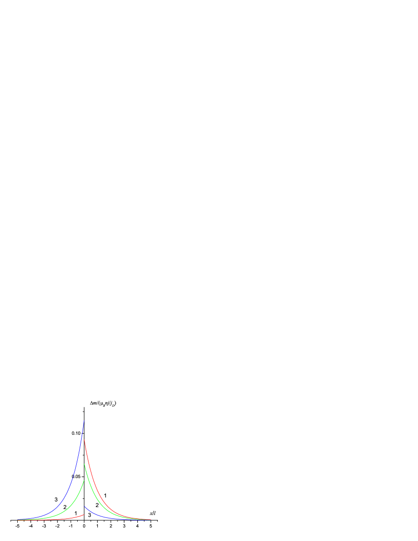
Figure 1: The nonequilibrium magnetization distribution (in dimensionless variables) at different values of the spin resistance ratio $\nu$: 1 — $\nu=10$ (red), 2 — $\nu=1$ (green), 3 — $\nu=0.1$ (blue). $Q=0.35,\;Q^{\prime}=0.15,\;l=l^{\prime},\;n=n^{\prime},\;j_{D}=j^{\prime}_{D},\;\chi=45^{\circ}$.

5 Spin accumulation resistance

The spin equilibrium disturbance contributes to the resistance of the system in study. We have

$$j_{\pm}=-\sigma_{\pm}\left(\frac{d\varphi}{dx}+\frac{1}{e}\frac{d\zeta_{\pm}}{dx}\right).$$ (26)

With Eqs. (5) and (16) taking into account,

$$\frac{d\varphi}{dx}=-\frac{1}{\sigma}\left[j+\frac{1}{e}\left(\sigma_{+}\frac{d\zeta_{+}}{dx}+\sigma_{-}\frac{d\zeta_{-}}{dx}\right)\right]=-\frac{1}{\sigma}\left[j+\frac{e}{2\mu_{B}}\left(D_{+}-D_{-}\right)\frac{dm}{dx}\right].$$ (27)

By integrating Eq. (27) over $x$ with potential drop at $x=0$ taking into account, we obtain

$$\varphi(-0)-\varphi(-L)+\varphi(L^{\prime})-\varphi(+0)=-\frac{j}{\sigma}L-\frac{e}{2\mu_{B}\sigma}\left(D_{+}-D_{-}\right)\Delta m(-0)$$

$$-\frac{j}{\sigma^{\prime}}L^{\prime}-\frac{e}{2\mu_{B}\sigma^{\prime}}\left(D^{\prime}_{+}-D^{\prime}_{-}\right)\Delta m^{\prime}(+0),$$ (28)

where $L,\,L^{\prime}$ are thicknesses of the contacting layers ($L\gg l,\;L^{\prime}\gg l^{\prime}$).

The total potential drop over the whole system is

$$U\equiv\varphi(-L)-\varphi(L^{\prime})=\left(\frac{L}{\sigma}+\frac{L^{\prime}}{\sigma^{\prime}}\right)j+\left[\varphi(-0)-\varphi(+0)\right]$$

$$+\frac{e}{2\mu_{B}}\left[\frac{1}{\sigma}\left(D_{+}-D_{-}\right)\Delta m(-0)-\frac{1}{\sigma^{\prime}}\left(D^{\prime}_{+}-D^{\prime}_{-}\right)\Delta m^{\prime}(+0)\right].$$ (29)

By equating the content of the first curly brackets in Eq. (3) to zero, we find the part of the potential drop at the interface:

$$\varphi(-0)-\varphi(+0)=\frac{1}{2e}\left(\zeta^{\prime}_{+}+\zeta^{\prime}_{-}-\zeta_{+}-\zeta_{-}\right)$$

$$=\frac{1}{e}(\bar{\zeta}^{\prime}-\bar{\zeta})+\frac{1}{2e}\left(\Delta\zeta^{\prime}_{+}+\Delta\zeta^{\prime}_{-}-\Delta\zeta_{+}-\Delta\zeta_{-}\right)=\frac{1}{e}(\bar{\zeta}^{\prime}-\bar{\zeta})$$

$$+\frac{e}{4\mu_{B}}\left[\left(\frac{D^{\prime}_{+}}{\sigma^{\prime}_{+}}-\frac{D^{\prime}_{-}}{\sigma^{\prime}_{-}}\right)\Delta m^{\prime}(+0)-\left(\frac{D_{+}}{\sigma_{+}}-\frac{D_{-}}{\sigma_{-}}\right)\Delta m(-0)\right].$$ (30)

By substituting Eq. (5) into (5), we get after some manipulations

$$U=U_{0}+\frac{e}{\mu_{B}}\left[\frac{Q\tilde{D}Z}{l}\Delta m(-0)-\frac{Q^{\prime}\tilde{D}^{\prime}Z^{\prime}}{l^{\prime}}\Delta m^{\prime}(+0)\right],$$ (31)

where

$$U_{0}=\left(\frac{L}{\sigma}+\frac{L^{\prime}}{\sigma^{\prime}}\right)j+\frac{1}{e}\left(\bar{\zeta}^{\prime}-\bar{\zeta}\right)$$ (32)

is the voltage in absence of the spin equilibrium breaking.

Substitution of Eqs. (23) and (24) into Eq. (31) gives

$$U=U_{0}+jZ\frac{\left(Q\cos\chi-Q^{\prime}\right)^{2}}{\nu+\cos^{2}\chi}.$$ (33)

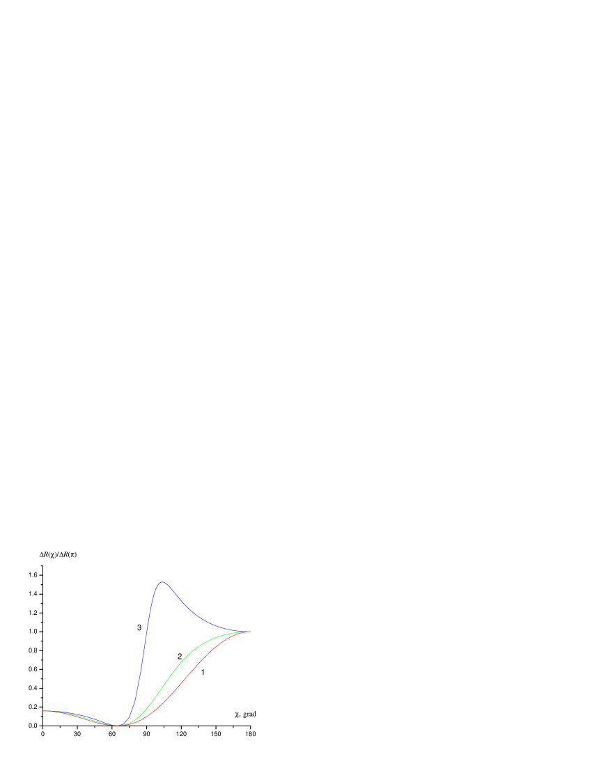
Figure 2: Spin accumulation resistance as a function of the angle $\chi$ between the layer magnetization vectors at different values of the spin resistance ratio $\nu$: 1 — $\nu=10$ (red), 2 — $\nu=1$ (green), 3 — $\nu=0.1$ (blue). $Q=0.35,\;Q^{\prime}=0.15$.

The contribution of spin accumulation to the resistance as a function of $\chi$ angle can be found:

$$\Delta R(\chi)\equiv\frac{U-U_{0}}{j}=ZZ^{\prime}\frac{(Q\cos\chi-Q^{\prime})^{2}}{Z+Z^{\prime}\cos^{2}\chi}.$$ (34)

The angular dependence of $\Delta R$ is shown in Fig. 2. Note that $\Delta R$ vanishes at $\chi=\arccos(Q^{\prime}/Q)$.

The results obtained may be considered as a generalization of those in Refs. [3, 6, 15] to the case of nonidentical noncollinear ferromagnets. Really, in Ref. [6] the contact potential drop was calculated, that is, in essence, the first square bracket in Eq. (5). On the other hand, in Ref. [15] the volume potential difference, that is the last square bracket in Eq. (5) was calculated. As it is seen from Eq. (5), we should sum the brackets to obtain the final result. In addition, we take an arbitrary angle $\chi$ instead of collinear orientation taken in Refs. [6] and [15].

Giant magnetoresistance (GMR) can be found from Eq. (34):

$$\mathrm{GMR}\equiv\frac{\Delta R(\pi)-\Delta R(0)}{\Delta R(\pi)}=\frac{4QQ^{\prime}}{(Q+Q^{\prime})^{2}}.$$ (35)

At $Q=Q^{\prime}$ we have $\Delta R(0)=0$, so that GMR takes its maximum value $\mathrm{GMR}=1$.

6 Conclusion

We show the longitudinal spin flux continuity at the junction interface follows directly from the spin transformation properties under the rotation of a quantization axis.

We derive for the first time the continuity conditions of mobile electron chemical potentials at the interface of two ferromagnetic junction layers having an arbitrary angle between their magnetization vectors. When the conditions were derived, the only statement was employed significantly, namely, the conservation low of the mobile electron energy flux density at the interface.

Electron magnetization distribution in the junction is calculated based on the boundary conditions derived. Matching parameter is discussed, which determine the spin flux penetration through the interface. The parameter may be treated as a ratio of the contacting layers spin resistances.

We show the disturbance of spin equilibrium at the interface leads to angle dependent shift of a contact potential drop and to spin accumulation magnetoresistance. The last effect was numerically estimated and the angles are found of minimal and maximal magnetoresistance.

References

• [1] B. Heinrich, Canad. J. Phys. 78, 161 (2000).
• [2] P. C. van Son, H. van Kempen, P. Wyder, Phys. Rev. Lett. 58, 2271 (1987).
• [3] T. Valet, A. Fert, Phys. Rev. B 48, 7099 (1993).
• [4] D. L. Smith, R. N. Silver, Phys. Rev. B 64, 045323 (2001).
• [5] B. C. Lee, J. Korean Phys. Soc. 47, 1093 (2005).
• [6] A. K. Zvezdin, K. A. Zvezdin, Bulletin of the Lebedev Physics Institute No. 8, 3 (2002).
• [7] Yu. V. Gulyaev, P. E. Zilberman, E. M. Epshtein, R. J. Elliott, J. Exp. Theor. Phys. 100, 1005 (2005).
• [8] L. D. Landau, E. M. Lifshitz, Quantum Mechanics (Non-Relativistic Theory), Pergamon Press, London, 1977.
• [9] L. Berger, Phys. Rev. B 54, 9353 (1996).
• [10] Y. Utsumi, Y. Shimizu, H. Miyazaki, J. Phys. Soc. Japan 68, 3444 (1999).
• [11] Yu. V. Gulyaev, P. E. Zilberman, E. M. Epshtein, R. J. Elliott, J. Commun. Technol. and Electronics 48, 942 (2003).
• [12] E. J. Elliott, E. M. Epshtein, Yu. V. Gulyaev, P. E. Zilberman, J. Magn. Magn. Mater. 271, 88 (2004).
• [13] M. Gulliere, Phys. Lett. A 54, 225 (1975).
• [14] A. A. Abrikosov, Fundamentals of the Theory of Metals, North-Holland Publ. Comp., Amsterdam, 1988.
• [15] S. Zhang, P. M. Levy, Phys. Rev. B 65, 052409 (2002).