Generalized switchable coupling for superconducting qubits using double resonance

Abstract

We propose a method for switchable coupling between superconducting qubits using double resonance. The inter-qubit coupling is achieved by applying near-resonant oscillating fields to the two qubits. The deviation from resonance relaxes the criterion of strong driving fields while still allowing for a fully entangling two-qubit gate. This method avoids some of the shortcomings of previous proposals for switchable coupling. We discuss the possible application of our proposal to a pair of inductively coupled flux qubits, and we consider the extension to phase qubits.

I Introduction

Superconducting systems are among the most likely candidates for the implementation of quantum information processing applications You1 . In order to perform multi-qubit operations, one needs a reliable method for switchable coupling between the qubits, i.e. a coupling mechanism that can be easily turned on and off. Over the past few years, there have been several theoretical proposals to achieve that goal Makhlin ; You2 ; Blais ; Averin ; Plourde1 ; Rigetti ; Liu1 ; Bertet ; Liu2 ; Niskanen , and initial experimental advances have been made Pashkin ; Johnson ; Berkley ; Yamamoto ; Izmalkov ; Xu ; McDermott ; Majer ; Plourde2 ; vdPloeg . The early proposals involved performing fast changes in the qubit parameters and taking the qubits out of their so-called optimal points Makhlin ; You2 or using additional circuit elements Blais ; Averin ; Plourde1 . Both approaches increase the complexity of the experimental setup and add noise to the system. Rigetti et al. Rigetti proposed a switchable coupling mechanism that is turned on by applying resonant oscillating fields to the qubits and employing ideas inspired by the double-resonance physics known from nuclear magnetic resonance (NMR) Hartmann ; Slichter . In their proposal the qubits are kept at their optimal points throughout the experiment, neglecting the oscillating deviations caused by the driving fields. In spite of its appealing minimal reliance on additional circuit elements, that proposal requires the application of large driving fields. Other authors later proposed alternative mechanisms that avoided that limitation while still using oscillating fields or oscillating circuit parameters to induce inter-qubit coupling Liu1 ; Bertet ; Liu2 ; Niskanen . Those most recent proposals, however, suffer from some limitations of their own, e.g. not being usable at the optimal point Liu1 or requiring additional circuit elements Bertet ; Liu2 ; Niskanen .

Here we propose a generalized version of the double-resonance method where the constraint on the driving amplitudes is substantially milder than that required for the proposal of Ref. Rigetti . Our proposal provides an alternative to experimentalists when deciding what is the most suitable coupling mechanism to use in their experimental setup.

It is worth noting from the outset that the term double resonance could be somewhat misleading in this context, since the mechanism discussed below requires only one resonance criterion, namely the one given in Eq. (6). However, we use it following similar mechanisms in the context of NMR Slichter .

The paper is organized as follows. In Sec. II we introduce the model system and review recent proposals for achieving switchable coupling. In Sec. III we derive our proposed coupling mechanism and consider some aspects of its operation. In Sec. IV we discuss the possible application of the proposal to realistic experimental setups that use inductively coupled flux qubits or capacitively coupled phase qubits. We conclude the discussion in Sec. V.

II Model system and previous proposals

We start by describing the system in general terms, and we defer the discussion of its physical implementation to Sec. IV. The system that we consider is composed of two qubits with fixed bias and interaction parameters. Oscillating external fields can then be applied to the system in order to perform the different gate operations. In other words, we consider the same system that was considered in Ref. Rigetti . The effective Hamiltonian of the system is given by:

$$\hat{H}=-\sum_{j=1}^{2}\left(\frac{\omega_{j}}{2}\hat{\sigma}_{z}^{(j)}+\Omega_{j}\cos\left(\omega_{j}^{\rm rf}t+\varphi_{j}\right)\hat{\sigma}_{x}^{(j)}\right)+\frac{\lambda}{2}\hat{\sigma}_{x}^{(1)}\hat{\sigma}_{x}^{(2)},$$ (1)

where $\omega_{j}$ is the energy splitting between the two states of the qubit labelled with the index $j$; $\Omega_{j}$, $\omega_{j}^{\rm rf}$ and $\varphi_{j}$ are, respectively, the amplitude, frequency and phase of the applied oscillating fields, $\lambda$ is the inter-qubit coupling strength, and $\hat{\sigma}_{\alpha}^{(j)}$ are the Pauli matrices with $\alpha=x,y,z$ and $j=1,2$. The eigenstates of $\hat{\sigma}_{z}$ are denoted by $|g\rangle$ and $|e\rangle$, with $\hat{\sigma}_{z}|g\rangle=|g\rangle$. Note that we shall set $\hbar=1$ throughout this paper.

In order for the qubits to be effectively decoupled in the absence of driving by the oscillating fields, we take $\lambda\ll\Delta$, where $\Delta=\omega_{1}-\omega_{2}$, and we have assumed, with no loss of generality, that $\omega_{1}>\omega_{2}$ and $\lambda>0$. Note that the absence of terms of the form $\hat{\sigma}_{z}^{(1)}\hat{\sigma}_{z}^{(2)}$ is also crucial to ensure effective decoupling. Let us also take $\Delta\ll\omega$, where $\omega$ represents the typical size of the parameters $\omega_{j}$. Since we will generally assume driving amplitudes $\Omega_{j}$ comparable to $\Delta$, the above condition will be crucial in neglecting the fast-rotating terms below, i.e. in making the rotating-wave approximation (RWA).

Single-qubit operations can be performed straightforwardly by a combination of letting the qubit state evolve freely, i.e. with $\Omega_{j}=0$, and irradiating it at its resonance frequency, i.e. taking $\omega_{j}^{\rm rf}=\omega_{j}$. Under the effect of resonant irradiation, Rabi oscillations in the state of the qubit occur with frequency $\Omega_{j}$.

Although a clear review of previous proposals is not possible without a detailed discussion, we summarize the ideas of those proposals briefly here. The proposal of Ref. Rigetti involves irradiating each of the two interacting qubits on resonance, i.e. taking $\omega_{j}^{\rm rf}=\omega_{j}$, and relies on one manifestation of double resonance Hartmann ; Slichter . The idea of the double resonance in that case is that not only is each qubit driven resonantly, but also the sum of the Rabi frequencies of the two qubits matches the difference between their characteristic frequencies (i.e. $\Omega_{1}+\Omega_{2}=\Delta$). After making two rotating-frame transformations and neglecting fast-rotating terms, i.e. performing two RWAs, one finds that the inter-qubit coupling term is no longer effectively turned off (note that those transformations are essentially a special case of the ones we shall give in Sec. III). One thus achieves switchable coupling between the qubits. That proposal was criticized, however, for requiring such large Rabi frequencies. The proposal of Ref. Liu1 uses an external field applied to one qubit at the sum of or difference between the characteristic frequencies of the two qubits in order to perform gate operations (e.g. $\omega_{1}^{\rm rf}=\omega_{1}-\omega_{2}$, $\Omega_{2}=0$). However, since all the relevant matrix elements, e.g. $\langle gg|\hat{\sigma}_{x}^{(1)}|ee\rangle$, with the eigenstates of the Hamiltonian in Eq. (1) vanish, the proposed method would not drive the intended transitions. One therefore needs to use a somewhat modified Hamiltonian, e.g. one that contains an additional single-qubit static term with a $\hat{\sigma}_{x}$ operator . In practice, that means biasing one of the qubits away from its optimal point in the case of charge or flux qubits. Since optimal-point operation is highly desirable in order to minimize decoherence, an alternative mechanism was proposed in Refs. Bertet ; Niskanen . In those proposals an additional circuit element that can mediate coupling between the qubits is added to the circuit design. That addition effectively makes the parameter $\lambda$ in Eq. (1) tunable, with its value depending on the bias parameters of the additional circuit element. One of those parameters is then modulated at a frequency that matches either the sum of or difference between the characteristic qubit frequencies. Clearly, since the driving term contains the operator $\hat{\sigma}_{x}^{(1)}\hat{\sigma}_{x}^{(2)}$, it can drive oscillations in the transition $|gg\rangle\leftrightarrow|ee\rangle$ or $|ge\rangle\leftrightarrow|eg\rangle$, even when both qubits are operated at their optimal points. As mentioned above, however, the use of additional circuit elements is undesirable, because of the increased circuit complexity and decoherence.

In the next section, we shall derive our proposal to couple the qubits by applying two external fields close to resonance with the interacting pair of qubits such that neither qubit is driven resonantly, but the sum of the (nonresonant) Rabi frequencies satisfies the double-resonance condition. Therefore, in some sense we relax the requirement that the driving amplitudes must be as large as $\Delta/2$, as is the case in Ref. Rigetti , and we make up for the resulting loss of frequency by adding the qubit-field frequency detuning to the double-resonance condition.

III Theoretical analysis

We now turn to the main proposal of this paper, namely driving oscillations between the states $|gg\rangle$ and $|ee\rangle$ by employing double resonance with non-resonant oscillating fields. We take the Hamiltonian in Eq. (1) and transform it as follows:

$$\hat{H}^{\prime}=\hat{S}_{1}^{\dagger}(t)\hat{H}\hat{S}_{1}(t)+i\frac{d\hat{S}_{1}^{\dagger}}{dt}\hat{S}_{1},$$ (2)

where

$$\hat{S}_{1}(t)=\exp\left\{i\sum_{j=1}^{2}\frac{\omega_{j}^{\rm rf}}{2}\hat{\sigma}_{z}^{(j)}t\right\}.$$ (3)

A solution of the Schrödinger equation $id|\Psi(t)\rangle/dt=\hat{H}|\Psi(t)\rangle$ can then be expressed as $\hat{S}_{1}(t)|\Psi^{\prime}(t)\rangle$, where $|\Psi^{\prime}\rangle$ satisfies the equation $id|\Psi^{\prime}(t)\rangle/dt=\hat{H}^{\prime}|\Psi^{\prime}(t)\rangle$. To simplify the following algebra, we take $\varphi_{1}=\varphi_{2}=0$. Neglecting terms that oscillate with frequency of the order of $\omega_{j}$, we find that

$$\hat{H}^{\prime}= -\sum_{j=1}^{2}\left(\frac{\delta\omega_{j}}{2}\hat{\sigma}_{z}^{(j)}+\frac{\Omega_{j}}{2}\hat{\sigma}_{x}^{(j)}\right)$$ (4)

$$+\frac{\lambda}{4}\bigg{(}\hat{\sigma}_{x}^{(1)}\hat{\sigma}_{x}^{(2)}\cos\delta\omega_{\rm rf}t+\hat{\sigma}_{y}^{(1)}\hat{\sigma}_{y}^{(2)}\cos\delta\omega_{\rm rf}t$$

$$\hskip 14.22636pt+\hat{\sigma}_{y}^{(1)}\hat{\sigma}_{x}^{(2)}\sin\delta\omega_{\rm rf}t-\hat{\sigma}_{x}^{(1)}\hat{\sigma}_{y}^{(2)}\sin\delta\omega_{\rm rf}t\bigg{)},$$

where $\delta\omega_{j}=\omega_{j}-\omega_{j}^{\rm rf}$, and $\delta\omega_{\rm rf}=\omega_{1}^{\rm rf}-\omega_{2}^{\rm rf}$. We now make a basis transformation in spin space from the operators $\hat{\sigma}$ to the operators $\hat{\tau}$ such that the time-independent terms in Eq. (4) are parallel to the new $z$-axis and the $y$-axis is not affected. Equation (4) can then be re-expressed as:

$$\hat{H}^{\prime}= -\sum_{j=1}^{2}\left(\frac{\tilde{\omega}_{j}}{2}\hat{\tau}_{z}^{(j)}\right)$$ (5)

$$+\frac{\lambda}{4}\bigg{(}\hat{\tau}_{x}^{(1)}\hat{\tau}_{x}^{(2)}\cos\theta_{1}\cos\theta_{2}\cos\delta\omega_{\rm rf}t+\hat{\tau}_{y}^{(1)}\hat{\tau}_{y}^{(2)}\cos\delta\omega_{\rm rf}t$$

$$\hskip 14.22636pt+\hat{\tau}_{y}^{(1)}\hat{\tau}_{x}^{(2)}\cos\theta_{2}\sin\delta\omega_{\rm rf}t-\hat{\tau}_{x}^{(1)}\hat{\tau}_{y}^{(2)}\cos\theta_{1}\sin\delta\omega_{\rm rf}t$$

$$\hskip 14.22636pt+\hat{A}\bigg{)},$$

where $\tilde{\omega}_{j}=\sqrt{\delta\omega_{j}^{2}+\Omega_{j}^{2}}$, the angles $\theta_{j}$ are defined by the criterion $\tan\theta_{j}=\Omega_{j}/\delta\omega_{j}$, and $\hat{A}$ contains terms in Eq. (4) that were not written out explicitly in Eq. (5) because they will soon be neglected. We now take the frequencies to match the criterion $\tilde{\omega}_{1}+\tilde{\omega}_{2}=\delta\omega_{\rm rf}$, or more explicitly

$$\sqrt{\delta\omega_{1}^{2}+\Omega_{1}^{2}}+\sqrt{\delta\omega_{2}^{2}+\Omega_{2}^{2}}=\Delta-\delta\omega_{1}+\delta\omega_{2},$$ (6)

where, as mentioned above, $\delta\omega_{j}=\omega_{j}-\omega_{j}^{\rm rf}$, and $\Delta=\omega_{1}-\omega_{2}$. We also take the two terms on the left-hand side of Eq. (6) to be comparable to one another. Taking the above condition allows us to simplify $\hat{H}^{\prime}$ with one more transformation. Using a similar procedure to that we used above for the first transformation, we now take

$$\hat{S}_{2}=\exp\left\{i\sum_{j=1}^{2}\frac{\tilde{\omega}_{j}}{2}\hat{\tau}_{z}^{(j)}t\right\},$$ (7)

and after neglecting terms that oscillate with frequency of order $\Delta$ we find that

$$\hat{H}^{\prime\prime}=\frac{\lambda}{16}(1-\cos\theta_{1})(1+\cos\theta_{2})\left\{\hat{\tau}_{y}^{(1)}\hat{\tau}_{y}^{(2)}-\hat{\tau}_{x}^{(1)}\hat{\tau}_{x}^{(2)}\right\}.$$ (8)

The reason why we can neglect the term $\hat{A}$ in the above transformation can be seen by observing that all the terms contained in $\hat{A}$ contain at least one $\hat{\tau}_{z}$ operator, and they oscillate with frequency $\delta\omega_{\rm rf}$. Therefore, even after the transformation, those terms will still oscillate with frequencies that are of the order of $\Delta$ (and amplitudes smaller than $\lambda$), meaning that their effects on the dynamics can be neglected in $\hat{H}^{\prime\prime}$, whose typical energy scale is a fraction of $\lambda$.

Equations (6) and (8) form the basis for the coupling mechanism that we propose in this paper. The Hamiltonian $\hat{H}^{\prime\prime}$ drives the transition $|gg\rangle\leftrightarrow|ee\rangle$ but does not affect the states $|ge\rangle$ and $|eg\rangle$ in the basis of the operators $\hat{\tau}$. Therefore, a single two-qubit gate that can be performed using the Hamiltonian $\hat{H}^{\prime\prime}$ and the set of all single-qubit transformations form a universal set of gates for quantum computing. Note that since the two-qubit gate is performed in the basis of the $\hat{\tau}$ matrices rather than the $\hat{\sigma}$ matrices, one needs to include in the pulse sequence the appropriate single-qubit operations before and after the two-qubit gate. Note also that if we take the special case $\cos\theta_{1}=\cos\theta_{2}=0$, i.e. $\delta\omega_{1}=\delta\omega_{2}=0$, we recover the corresponding case in the results of Ref. Rigetti .

A first look at Eq. (8) shows that one can achieve faster gate operation than in the special case $\cos\theta_{1}=\cos\theta_{2}=0$ by choosing $\cos\theta_{1}$ to be negative and $\cos\theta_{2}$ to be positive. In other words, instead of using the special case of resonant driving ($\delta\omega_{1}=\delta\omega_{2}=0$) one chooses $\delta\omega_{1}$ to be negative and $\delta\omega_{2}$ to be positive (i.e., $\omega_{1}^{\rm rf}>\omega_{1}$ and $\omega_{2}^{\rm rf}<\omega_{2}$). However, inspection of Eq. (6) while noting that $\sqrt{\delta\omega_{j}^{2}+\Omega_{j}^{2}}<|\delta\omega_{j}|+\Omega_{j}$ shows that one would then have to increase at least one of the frequencies $\Omega_{j}$ above the value $\Delta/2$ in order to satisfy Eq. (6) with that choice of $\delta\omega_{1}$ and $\delta\omega_{2}$. Since we started with the motivation of finding an alternative double-resonance method that works with smaller values of $\Omega_{j}$, we focus on the opposite case, namely $\delta\omega_{1}>0$ and $\delta\omega_{2}<0$, and we accept the resulting reduction in gate operation speed. Starting from the special case $\delta\omega_{1}=\delta\omega_{2}=0$ and moving in the direction given above, we find that both $\Omega$s can now be reduced below the value $\Delta/2$ while satisfying Eq. (6).

It is worth pausing here to comment on the higher-order effects that we have neglected in making the two RWAs. The second-order shifts that we have neglected in making our first RWA, i.e. the Bloch-Siegert shifts, are of order $\Omega_{j}^{2}/\omega_{j}$ CohenTannoudji . That energy scale is not obviously smaller than the inter-qubit coupling strength $\lambda$. One might therefore suspect that those shifts will prohibit the performance of the proposed method. That is not the case, however, since those shifts only modify the values of the required driving frequencies and amplitudes, as we shall demonstrate with numerical simulations in Sec. IV. There we shall take the case where $\Delta^{2}/\omega_{1}=2\lambda$, and we shall show that full oscillations between the states $|gg\rangle$ and $|ee\rangle$ can still be obtained when the shifts are properly taken into account. Other frequency shifts that result from our approximations, and possibly other experiment-specific shifts, also affect the required driving frequencies and amplitudes. We will not attempt to give analytic expressions for those shifts. However, we will take them into account by numerically scanning the driving amplitudes to achieve optimal gate operation.

We now ask the question of how low can $\Omega_{j}$ be chosen to be. In principle, Eq. (6) can still be satisfied by taking $\Omega_{j}$ to be very small and taking $\delta\omega_{1}\approx\Delta/4$, $\delta\omega_{2}\approx-\Delta/4$. Note, however, that the frequency of gate operations is given by the coefficient in Eq. (8), namely $\lambda(1-\cos\theta_{1})(1+\cos\theta_{2})/16$. That coefficient therefore determines the width of the resonance, or in other words, the error tolerance in driving amplitudes from the resonance criterion (Eq. 6) ResonanceWidth . One is therefore restricted to using values of $\theta_{1}$ and $\theta_{2}$ such that the above coefficient is larger than the accuracy of the available pulse generators. Furthermore, taking the inverse of the frequency determines the period of oscillations in the doubly rotating frame, or in other words, the time required to perform a two-qubit gate operation. Since the decoherence time sets an upper limit on how slowly one can perform the gate operations, that consideration provides another restriction on the allowed values of $\theta_{1}$ and $\theta_{2}$. An experimentalist must therefore take the two above considerations into account, along with any restriction they have on the maximum usable driving amplitudes, in order to determine the window of parameters where the coupling mechanism can be realized. The parameters can then be fine-tuned within that window for optimal results.

As an added perspective to help visualize the resonance criterion, we show in Fig. 1 the relevant energy-level structure. One can compare this figure to Fig. 2 in Ref. Rigetti . In that case, the on-resonance Rabi frequencies provide all of the energy splitting (i.e. $\tilde{\omega}_{1}$ and $\tilde{\omega}_{2}$) required to satisfy the resonance criterion. In the present case, the energy levels involved in the frequency matching are already brought closer to each other by the facts that (1) the difference $\omega_{1}^{\rm rf}-\omega_{2}^{\rm rf}$ is smaller than the difference $\omega_{1}-\omega_{2}$ and (2) the detuning of each driving field from its corresponding qubit brings the relevant levels even closer to each other. It would appear from Fig. 1 that the resonance criterion can be satisfied with arbitrarily small driving amplitudes and the proper choice of $\omega_{1}^{\rm rf}$ and $\omega_{2}^{\rm rf}$. As was discussed above, however, the matrix element (in the dressed-state picture) coupling the relevant energy levels becomes very small in that case, leading to the undesirable situation of high required accuracy in the driving fields and slow gate operation.

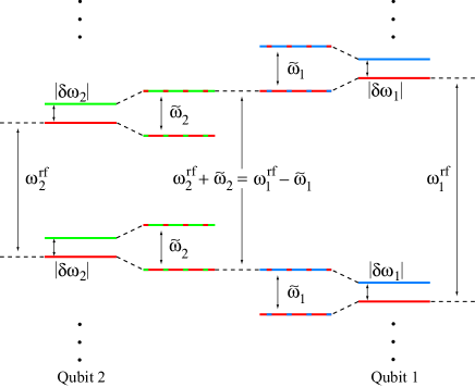
Figure 1: (color online) The energy level diagrams of the two qubits in the dressed-state picture. The resonance criterion is satisfied when the smallest energy difference between two adjacent manifolds of qubit 1 states becomes equal to the largest energy difference between two adjacent manifolds of qubit 2 states. Note that $\tilde{\omega}_{j}=\sqrt{\delta\omega_{j}^{2}+\Omega_{j}^{2}}$.

We reiterate that care must be taken in using the term double resonance in describing the coupling mechanism discussed above. However, since it seems that the term is used to describe a number of distinct phenomena in NMR Slichter , some of which bear resemblance to the one discussed here, we have followed that broad definition of the term. Note, in particular, that the mechanism discussed above requires only one resonance condition, namely the one given in Eq. (6). Neither applied field has to be resonant with its corresponding qubit, provided that they are kept close enough to resonance that the two-qubit gate can be performed in reasonable time.

IV Experimental considerations

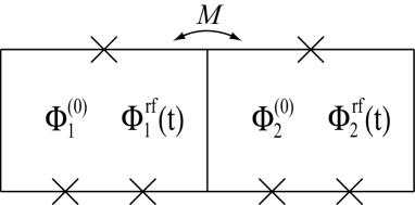
Figure 2: Two inductively coupled flux qubits. The symbols $\times$ represent Josephson junctions. The static and oscillating externally applied magnetic fluxes, $\Phi_{j}^{(0)}$ and $\Phi_{j}^{\rm rf}(t)$, are used to control the two qubits. The interaction is mediated by the mutual inductance $M$ between the two qubit loops.

In the above discussion, we have not specified what kind of qubits we consider. Our results therefore apply to any kind of qubit where the effective Hamiltonian of Eq. (1) describes the two-qubit system. Because of its relevance to current experimental attempts to achieve switchable coupling between superconducting qubits, we now focus on the case of two inductively coupled flux qubits, as shown in Fig. 2 Plourde2 ; Harrabi . Since the truncation of the full Hamiltonian to the effective Hamiltonian of Eq. (1) has already been discussed by several authors (see e.g. Ref. Liu1 ) and it is not central to our discussion, we do not include it here.

In experiments on flux qubits, the individual qubits typically have $\omega_{j}\approx(2\pi)\times 5$ GHz (note that the exact value is not completely controllable during fabrication, with the uncertainty reaching 0.5-1 GHz in some experiments) Plourde2 ; Harrabi ; Chiorescu . The inter-qubit coupling strength $\lambda$ can be taken to be around $(2\pi)\times 0.1$ GHz. The highest achievable on-resonance Rabi frequencies $\Omega_{j}$ are in the range of several hundred MHz to 1 GHz (times $2\pi$). The achievable Rabi frequencies are therefore large enough when compared with the naturally (i.e., uncontrollably) occurring inter-qubit detuning $\Delta$, suggesting that it might be possible to implement the proposal of Ref. Rigetti with the above qubit design. However, additional difficulties that we have not discussed in Sec. III arise in different experimental setups.

One experimental difficulty arises when $\Delta$ is 0.5-1 GHz Harrabi . In that case, the required Rabi frequencies are large enough to excite higher states outside the truncated qubit basis, in addition to exciting other modes in the circuit. One would therefore ideally want to avoid using the highest values of $\Omega_{j}$ cited above ($\sim$ 0.5 GHz). Taking intermediate values of $\cos\theta$ between 0 and 1, the required Rabi frequencies can be reduced substantially, and the two-qubit gate operation can still be performed in a time of the order of a few hundred nanoseconds. That time scale is smaller than the qubit decoherence times (typically 1-3 $\mu$s), which means that a simple two-qubit quantum gate operation could be observable in the near future. Clearly, an increase in the decoherence times would be highly desirable in order to achieve longer sequences of gate operations.

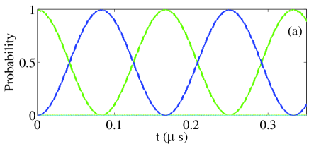
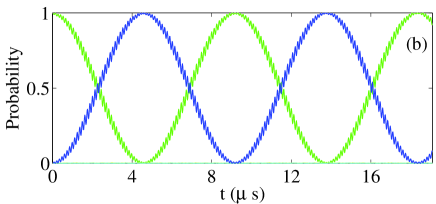
Figure 3: (color online) The occupation probabilities of the four eigenstates as functions of time. The blue (black), green (gray), cyan and yellow lines (the last two are essentially zero and barely visible) correspond, respectively, to the states $|ee\rangle$, $|gg\rangle$, $|ge\rangle$ and $|eg\rangle$. The initial state is $|gg\rangle$, $\omega_{1}/2\pi$=5 GHz, $\omega_{2}/2\pi$=4 GHz, and $\lambda/2\pi$=0.1 GHz. The driving frequencies and amplitudes include shifts caused by higher-order corrections. In both (a) and (b), $\omega_{j}^{\rm rf}$ includes the Bloch-Siegert shift $\Omega_{j}^{2}/4\omega_{j}$. In (a) $\theta_{1}=\pi-\theta_{2}=\pi/3$, and the $\Omega$s (approximately $2\pi\times$ 0.29 GHz) were shifted by 0.5% to correct for shifts in our second RWA. In (b) $\theta_{1}=\pi-\theta_{2}=\pi/8$, and the $\Omega$s (approximately $2\pi\times$ 0.1 GHz) were shifted by 6.38% ManualShifts .

We have performed numerical simulations to show that the two-qubit gate can be performed for a wide range of values of $\theta_{1}$ and $\theta_{2}$ (note that smaller values of $\theta_{1}$ correspond to smaller driving amplitudes, and that we take $\theta\equiv\theta_{1}=\pi-\theta_{2}$). The simulations are performed by solving the time-dependent Schrödinger equation with the Hamiltonian of Eq. (1). We therefore make the two-level system approximation in describing each qubit. The results are shown in Fig. 3. If we take realistic experimental parameters and $\theta=\pi/3$, which corresponds to a reduction in the required driving amplitudes by a factor of about two, and we take the qubit to be initially in the state $|gg\rangle$, we can see that the occupation probability oscillates between the states $|gg\rangle$ and $|ee\rangle$ with negligible errors and a very reasonable oscillation period (note that since we are considering a simple experiment designed to provide a proof-of-principle demonstration of switchable coupling, errors of the order of 1% are negligible). In Fig. 3(b), we take the same experimental parameters, but we now take $\theta=\pi/8$, which corresponds to a reduction in the required driving amplitudes by a factor of five. We can see that full oscillations can still be achieved when taking into account the shifts in the required driving fields. However, the period of oscillations and the required accuracy in tuning the driving amplitude are now outside the experimentally desirable range. These results therefore agree with the statement made above that one should look for the ideal point of gate operation, i.e. reduce the amplitudes of the driving fields just enough to reduce the errors caused by them to acceptable levels.

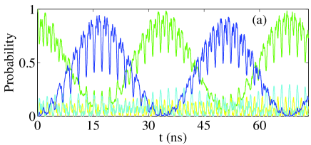
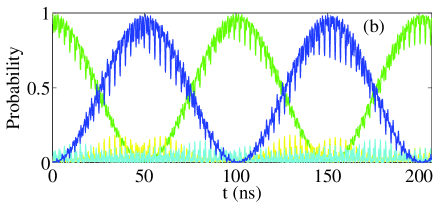
Figure 4: (color online) Same as in Fig. 3, but including the effects of 100% crosstalk (the occupation probabilities of the states $|ge\rangle$ and $|eg\rangle$ are now more visible than in Fig. 3, but they are still small compared to those of the states $|gg\rangle$ and $|ee\rangle$). In (a) $\theta_{1}=\theta_{2}=\pi/2$, the $\omega^{\rm rf}$s were shifted by 0.5%, and the $\Omega$s ($2\pi\times$ 0.49 GHz) were shifted by 2%. In (b) $\theta_{1}=\pi-\theta_{2}=\pi/3$, the $\omega^{\rm rf}$s were shifted by 2.5%, and the $\Omega$s (approximately $2\pi\times$ 0.29 GHz) do not include any shifts from the expressions of Sec. III.

Another experimental issue that we have not addressed above arises in the case of crosstalk, i.e. when each qubit feels the microwave signal intended for the other qubit Plourde2 . In other words, the Hamiltonian describing the system includes additional terms of the form $\beta\Omega_{j}\cos(\omega_{j}^{\rm rf}t+\varphi_{j})\sigma_{x}^{(j^{\prime})}$, where $j\neq j^{\prime}$, and the coefficient $\beta$ quantifies the amount of crosstalk. If the amplitudes of the applied fields are small, a microwave signal that is resonant with one qubit will not affect the other qubit. However, if the Rabi frequencies are comparable to the inter-qubit detuning, e.g. when $\Omega_{2}=(\omega_{1}-\omega_{2}^{\rm rf})/2$ and $\beta\sim 1$, crosstalk cannot be neglected. In our method the ratio $\Omega_{2}/(\omega_{1}-\omega_{2}^{\rm rf})$ is equal to $\sin\theta/(2+\cos\theta)$, suggesting that the harmful effects of crosstalk could be reduced by decreasing $\theta$. In fact, we have verified with numerical simulations that the errors caused by crosstalk are reduced by using our method, as shown in Fig. 4. Some of the shifts to the driving frequencies and amplitudes were determined manually by looking for optimal results. Note that the driving parameters corresponding to Fig. 4(b) also drive oscillations between the states $|eg\rangle$ and $|ge\rangle$. However, combining the two driven transitions still describes effective coupling between the qubits. The period of oscillations in Fig. 4(b) is about 100 ns, suggesting that an experimental demonstration of the coupling should be possible even in the presence of 100% crosstalk.

Finally, let us make a few remarks about the possible implementation of our method to capacitively coupled phase qubits Berkley ; McDermott . It is perhaps clearest to start by noting a point that is not directly related to the procedure of implementing our proposal: one of the main considerations in charge and flux qubits, namely the question of optimal-point operation, is rather irrelevant to the study of phase qubits, at least in the usual sense of using eigenstates with special symmetries to minimize decoherence. The phase qubit is simply a single Josephson junction controlled by a bias current. The static part of the bias current determines the qubit splittings $\omega_{j}$, whereas the amplitude of the oscillating part of the bias current determines the Rabi frequencies $\Omega_{j}$ Martinis . If one now takes two capacitively coupled phase qubits, one finds that the coupling term has the form $\hat{\sigma}_{y}^{(1)}\hat{\sigma}_{y}^{(2)}$ sigmaxy . If we now take the phases of the oscillating fields $\varphi_{1}=\varphi_{2}=\pi/2$, we can follow the derivation of Sec. III and obtain the same results. In phase qubits the qubit splittings $\omega_{j}$ are typically a few GHz (times $2\pi$), and unlike flux qubits those splittings can be tuned using the bias current during the experiment. Rabi frequencies can reach a few hundred MHz, and the coupling strength can be taken to be $(2\pi)\times$ 0.1 GHz, giving essentially the same values for the parameters as discussed above for flux qubits. We finally note that the driving fields are supplied through the bias current rather than through external fields, which means that crosstalk is not a problem with phase qubits. Realization of our proposal, or even that of Ref. Rigetti , should therefore be possible with capacitively coupled phase qubits.

V Conclusion

We have derived a generalized double-resonance method for switchable coupling between qubits. The qubits are driven close to resonance such that the sum of their Rabi frequencies is equal to the difference between the frequencies of the driving fields. Our proposal with nonresonant driving of the qubits relaxes the constraint on the resonant-driving proposal, i.e. that of Ref. Rigetti , requiring large driving amplitudes. We have compared the operation of resonant and nonresonant driving. Although our proposal can be applied to any kind of qubits, we have discussed in some detail its possible application to the special, but experimentally relevant, case of inductively coupled superconducting flux qubits. We have also considered the possible extension to the case of capacitively coupled phase qubits.

- (1) For recent reviews of the subject, see e.g. Y. Makhlin, G. Schön, and A. Shnirman, Rev. Mod. Phys. 73, 357 (2001); J. Q. You and F. Nori, Phys. Today 58 (11), 42 (2005); G. Wendin and V. Shumeiko, in Handbook of Theoretical and Computational Nanotechnology, ed. M. Rieth and W. Schommers (ASP, Los Angeles, 2006).
- (2) Y. Makhlin, G. Schön, and A. Shnirman, Nature 398, 305 (1999).
- (3) J. Q. You, J. S. Tsai, and F. Nori, Phys. Rev. Lett. 89, 197902 (2002); J. Q. You, J. S. Tsai, and F. Nori, Phys. Rev. B 68, 024510 (2003).
- (4) A. Blais, A. Maassen van den Brink, and A. M. Zagoskin, Phys. Rev. Lett. 90, 127901 (2003)
- (5) D. V. Averin and C. Bruder, Phys. Rev. Lett. 91, 057003 (2003).
- (6) B. L. T. Plourde, J. Zhang, K. B. Whaley, F. K. Wilhelm, T. L. Robertson, T. Hime, S. Linzen, P. A. Reichardt, C.-E. Wu, and J. Clarke, Phys. Rev. B 70, 140501(R) (2004).
- (7) C. Rigetti, A. Blais, and M. Devoret, Phys. Rev. Lett. 94, 240502 (2005).
- (8) Y.-X. Liu, L. F. Wei, J. S. Tsai, and F. Nori, Phys. Rev. Lett. 96, 067003 (2006).
- (9) P. Bertet, C. J. P. M. Harmans, and J. E. Mooij, Phys. Rev. B. 73, 064512 (2006).
- (10) Y.-X. Liu, L. F. Wei, J. S. Tsai, and F. Nori, cond-mat/0509236.
- (11) A. O. Niskanen, Y. Nakamura, and J. S. Tsai, Phys. Rev. B 73, 094506 (2006).
- (12) Yu. A. Pashkin, T. Yamamoto, O. Astafiev, Y. Nakamura, D. V. Averin and J. S. Tsai, Nature 421, 823 (2003).
- (13) P. R. Johnson, F. W. Strauch, A. J. Dragt, R. C. Ramos, C. J. Lobb, J. R. Anderson, and F. C. Wellstood, Phys. Rev. B 67, 020509(R) (2003).
- (14) A. J. Berkley, H. Xu, R. C. Ramos, M. A. Gubrud, F. W. Strauch, P. R. Johnson, J. R. Anderson, A. J. Dragt, C. J. Lobb, and F. C. Wellstood, Science 300, 1548 (2003).
- (15) T. Yamamoto, Yu. A. Pashkin, O. Astafiev, Y. Nakamura, and J. S. Tsai, Nature 425, 941 (2003).
- (16) A. Izmalkov, M. Grajcar, E. Il’ichev, Th. Wagner, H.-G. Meyer, A. Yu. Smirnov, M. H. S. Amin, A. Maassen van den Brink, and A. M. Zagoskin, Phys. Rev. Lett. 93, 037003 (2004).
- (17) H. Xu, F. W. Strauch, S. K. Dutta, P. R. Johnson, R. C. Ramos, A. J. Berkley, H. Paik, J. R. Anderson, A. J. Dragt, C. J. Lobb, and F. C. Wellstood, Phys. Rev. Lett. 94, 027003 (2005).
- (18) R. McDermott, R. W. Simmonds, M. Steffen, K. B. Cooper, K. Cicak, K. D. Osborn, S. Oh, D. P. Pappas, and J. Martinis, Science 307, 1299 (2005).
- (19) J. B. Majer, F. G. Paauw, A. C. J. ter Haar, C. J. P. M. Harmans, and J. E. Mooij, Phys. Rev. Lett. 94, 090501 (2005).
- (20) B. L. T. Plourde, T. L. Robertson, P. A. Reichardt, T. Hime, S. Linzen, C.-E. Wu, and J. Clarke, Phys. Rev. B 72, 060506(R) (2005).
- (21) S. H. W. van der Ploeg, A. Izmalkov, A. Maassen van den Brink, U. Huebner, M. Grajcar, E. Il’ichev, H.-G. Meyer, A. M. Zagoskin, cond-mat/0605588.
- (22) S. R. Hartmann and E. L. Hahn, Phys. Rev. 128, 2042 (1962).
- (23) See, e.g., C. P. Slichter, Principles of Magnetic Resonance (Springer, Berlin, 1996).
- (24) C. Cohen-Tannoudji, J. Dupont-Roc, and G. Grynberg, Atom-Photon Interactions (Wiley, New York, 1992).
- (25) This reduction in resonance width is given by the factor . For fixed relative errors in , the relative errors in are proportional to , reflecting the angle between the rotation axes of and . Noting that the ratio decreases with decreasing , we find that the allowed errors in also decrease with decreasing .
- (26) K. Harrabi, unpublished results.
- (27) I. Chiorescu, Y. Nakamura, C. J. P. Harmans, and J. E. Mooij, Science 299, 1869 (2003).
- (28) Note that the values of the manually obtained shifts are included here to demonstrate the required level of accuracy in the driving fields. They are not intended to suggest that any other physical effects in the experiment are expected to be smaller in size than those shifts.
- (29) For a discussion of the derivations, see J. M. Martinis, S. Nam, J. Aumentado, K. M. Lang, and C. Urbina, Phys. Rev. B 67, 094510 (2003).
- (30) The fact that the operators describing the coupling of the qubits to the external fields () and those describing the inter-qubit interaction () are different can be understood by observing that the bias current couples to the phase operator, whereas capacitive coupling is mediated by the charge operator.