Delayed Random Walks and Control

Abstract

Issues of resonance that appear in non-standard random walk models are discussed. The first walk is called repulsive delayed random walk, which is described in the context of a stick balancing experiment. It will be shown that a type of ”resonant” effect takes place to keep the stability of the fixed point better with tuned bias and delay. We also briefly discuss the second model called sticky random walk, which is introduced to model string entanglement. Peculiar resonant effects with respect to these random walks are presented.

(Published in Flow Dynamics: The Second International Conference on Flow Dynamics (M.Tokuyama and S. Maruyama eds.), AIP Conference Proceedings Vol. 832, pp. 487–491 (Melville, New York, 2006). )

I Introduction

A combination of non-linear dynamics and noise gives rise to the phenomena called stochastic resonance, which has been investigated actively longtin2 ; moss ; collins ; bulsara ; gam . The phenomena has been claimed to appear in a wide variety of things, such as climate change and neural information processing. The main theme of this paper is this type of phenomena in the context of non-standard random walks that we have proposed: repulsive ohira-hosaka04 and sticky. The former random walk was mainly derived from a stick balancing experimentcabrera-milton02 ; cabrera04 ; cabrera-etal04 , while the latter tries to model string entanglement. With both random walks, we observed rather unexpected phenomena that can be viewed as resonance. In the following, we describe each model and its associated behavior.

II Repulsive Delayed Random Walk

II.1 Model

As a mathematical framework to investigate the systems with noise and delay, delayed random walk has been proposed and studiedohira-milton95 ; ohira97 ; ohira-yamane00 . This is a random walk whose transition probability depends on its position at a fixed time interval in the past. The focus has been placed on the model which has an attractive bias to a single point. This stable case has been applied to such processes like posture control collins-deluca94 . Analytically, the attractive delayed random walk model has shown such behaviors like an oscillatory correlation function with increasing delay.

However, as the attractive model is not suitable to model the unstable situation we mentioned above, we discuss a delayed random walk which has a repulsive point. We can consider many different possibilities, but here we consider one-dimensional discrete time and step random walk with the origin as a repulsive point. Mathematically, we can define our model as follows. Let the position of the random walker at time step $t$ given by $X(t)$ and the fixed point set at the origin, $X=0$. The delayed random walk is defined by the following conditional probabilities.

$$P(X(t+1)=X(t)+1|X(t-\tau)>0) = p$$ (1)

$$P(X(t+1)=X(t)+1|X(t-\tau)=0) = {1\over 2}$$ (2)

$$P(X(t+1)=X(t)+1|X(t-\tau)<0) = 1-p,$$ (3)

where $0<p<1$ and $\tau$ is the delay. With delay, the walker refers to its position in the past to decide on the bias of his next step. The attractive model is the case of $p<0.5$, where the origin becomes attractive with no delay, $\tau=0$. On the other hand $p>0.5$ gives the repulsive case which we shall discuss for the rest of this paper.

Though this appears to be a little change of definition from the attractive case, we observe a very different behavior from the attractive case. Most of all, as the walker escapes away from the origin, we do not have a stationary probability distribution. This makes analytical treatment of this repulsive model more difficult as compared to the attractive case, particularly with non-zero delay. Our investigation in this paper is done by computer simulation. The most notable feature of this model is that we can find an optimal combination of the bias $p$ and $\tau$ where the random walker can be kept around the origin for a longest duration.

II.2 Analysis and Simulation Results

As in the case of stick balance experiment, one of the main interests is how long the walker can be kept around the repulsive fixed point. We investigated this by focusing on an average first passage time $L$ to reach a certain position (a limit point $\pm X^{*},X^{*}>0$) away from the origin. In other words, we measured the average time for the walker starting from the origin to reach the limit point for the first time as we changed parameters in the model. The longer average first passage time indicates slower diffusion, which corresponds to the situation of longer stick balancing.

For the case of zero delay with the bias $p$, we can find an analytical result for this average first passage time $L$ to reach the limit point $\pm X^{*}$ as

$$L=2\left({q\over{q-p}}\right)\left({{1-\left({q\over p}\right)^{X^{*}}}\over{1-{q\over p}}}\right)+{X^{*}\over{p-q}},\quad(p\neq 0.5),$$ (4)

where we have set $q\equiv 1-p$. For the case of simple (symmetric) random walk with $p=q=0.5$, this result reduces to an even simpler form.

$$L=(X^{*})^{2}.$$ (5)

For the case of non-zero delay, such analytical result is yet to be obtained and computer simulation is used. We considered an ensemble of 10000 walkers. The initial condition is set so that the walker performs a normal random walk with no bias $p=0.5$ for the duration of $t=(-\tau,0)$. The walker’s position at $t=0$ is set as the origin $X=0$. The limit point is set at $\pm X^{*}$. We measure the number of steps for each walker to go from the origin to $\pm X^{*}$ and average them. We performed computer simulations for various bias $p$ and delay $\tau$.

Some sample results are shown in Figure 1. The most notable features of these graphs are the peaks in the graph, indicating that the slowest diffusion appears at certain optimal values of $\tau$ given bias $p$. In other words, the walker is most stabilized around the origin with appropriate non-zero delay. This is rather unexpected result contrary to the normal notion associated with effects of feedback delay, where longer delay increasingly de-stabilize systems. Here, appropriate combination of bias and delay time is inducing more stability.

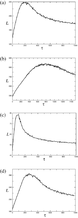
Figure 1: Average first passage time $L$ as we change $\tau$. The value of parameters $(p,{X^{*}})$ are (a) $(0.6,30)$, (b) $(0.6,100)$, (c) $(0.8,30)$, and (d) $(0.8,100)$.

In order to gain more insight into this phenomenon, we look for an approximate analytical expression, which is found to be given by the following expression

$$L(\tau)=(1+\alpha\tau_{n}{e^{-\beta\tau_{n}}})L(\tau=0).$$ (6)

Here $\alpha$ and $\beta$ are parameters and ${\tau_{n}}$ is a normalized delay given as follows.

$${\tau_{n}}\equiv\tau{p-q\over{X^{*}}}.$$ (7)

This normalization uses a characteristic time dividing the distance $X^{*}$ by an average velocity of the walker $p-q$. Hence ${\tau_{n}}$ is a non-dimensionalized parameter as well.

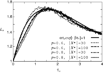
Figure 2: Normalized average first passage time $L_{n}\equiv{L(\tau)\over L(\tau=0)}$ as we change normalized delay $\tau_{n}$. The parameter sets $(p,{X^{*}})$ plotted are $(0.6,30)$, $(0.6,100)$, $(0.8,30)$, and $(0.8,100)$

Figure 2 shows this analytical approximation and the result of computer simulation. We see that the curves for various $(p,{X^{*}})$ overlaps quite well with the analytical curve with appropriately chosen parameters of $\alpha=1.27$ and $\beta=0.67$. We also notice that the peak height is approximately 1.7 times the average first passage time of zero delay case.

II.3 Delayed Stochastic Control

These theoretical results imply that systems can reach a better balancing performance if an appropriate amount of fluctuation is added given the feedback or reaction delay. We have termed this type of control, which is different from standard feedback or predictive ones, as delayed stochastic control. We performed the following experiment to gain some insight into the existence or utilization of this control scheme. We asked the subjects to sit on a chair and balance a stick, as in the previous stick balancing experiment. But, this time, the subjects were allowed to move their bodies, not just their arms, as they tried to balance the stick. One way to do this is to hold an object with the other hand and move it (Figure 3). Another way is to move their legs. We measured the time for which they could keep the sticks balanced, and compared it with the normal non-movement situations. Out of the six subjects we tested, three subjects showed notable improvement in balancing by reaching their own optimal level of movement (Figure 4).

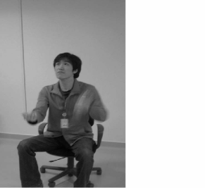
Figure 3: Picture of a subject balancing a stick on one hand while moving an object in the other.

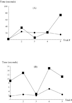
Figure 4: (A) Example of improvement on balancing tasks with (square) and without (dot) moving an object. The subject was given 5 trials without previous practice. By the 5th trial, the improvement was significant. (B) Another subject practiced for a few hours. Here, again improvement with moving the object was evident.

Some practice was needed for these subjects to reach this better performance. We believe that the subjects were tuning the appropriate level of fluctuation given their reaction times and prediction accuracy. Even though more thorough data needs to be collected, these results may be one supporting example of delayed stochastic control.

III Sticky Random Walk

III.1 Model

Entangled strings is something we commonly observe. For example, wires for electrical appliances or communication network cords sometimes require us to disentangle them. We describe here a concept of sticky random walk we used to gain some insight into this phenomenon. The model is simple. The strings are represented by the trajectory of a random walker. This random walker leaves sticks or marks at certain time intervals. Therefore, a string is represented by this trajectory with these marks on it. By sending out multiple sticky random walkers, we obtained multiple sticky strings. Furthermore, a string is considered as entangled with another when these marks overlap at the same site in space, and not when they are simply crossed. Thus, the string is considered more sticky when there are more marks on it.

We tested a situation having multiple sticky strings in a bounded two-dimensional square grid by sending out sticky random walks in this space. These random walks are discrete time, discrete space walks moving one step to its neighboring grid points. They are bounded by the edge of the square grid. We then pick one string randomly and count the number of strings either directly or indirectly entangled to that string. Indirect entanglement indicates that two strings are entangled through others, i.e., two strings can reach each other by following the chain of directly entangled strings. We performed simulation experiments with various conditions on the number of strings, the number of marks on each string, the length of each string, and the size of the two-dimensional square grid. In particular, we asked the question, if we compare the situation of having more strings with fewer marks and that of having fewer strings with more marks, while keeping the total number of marks in the space constant, which situation gives rise to more entanglement?

III.2 Simulation Results

We kept the total number of sticky marks $R$ and the length of each string $L$ as fixed, and we varied the number of strings $S$ and marks on each string $M$ so that $R=M\times S$. The number of entangled strings was measured both in numbers $E$ and in ratio $e={E\over S}$. Each part of the data is an average over 100 trials, with various space for $N$ by $N$ square grid. The representative results are shown in Figure 5. We found that an optimal combination of $S$ and $M$ exists. It is given as the highest peak in these graphs. This means that these strings are most entangled when the level of stickiness and the number of strings are optimally tuned. Even more unexpectedly, this optimal combination is independent of the space size $N$ for the ratio $e$. When $N$ is sufficiently large, it is also independent with respect to $E$ as well. Though it differs from the standard form of stochastic resonance, randomness in the motion of the walkers plays a role in bringing about this resonant behavior. Whether or not this behavior can happen in a real situation requires experimental tests.

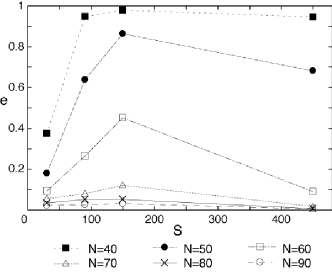
Figure 5: Average ratio, $e$, of entangled strings $e$ as number of marks on each string is changed. The length of each string is set at $L=60$, and the total number of marks is set at $R=1800$. Each line corresponds to a square lattice size $N$.

IV Discussion

We discussed two non-standard models of stochastic resonance. As a related subject, a binary bit model that shows resonance with noise and delay are proposed and studied ohira-sato ; tsimring . This phenomena was observed in an experiment with solid state laser masoller .

Our investigations here with respect to these resonance with random walks are still in the beginning stages. However, they already produced quite unexpected results. Further analysis as well as application with real systems could lead to some additional interesting insights.

Acknowledgments

We thank Dr. Juan Luis Cabrera and Prof. John G. Milton for their insightful comments. TH was a Research Fellow of the Japan Society for the Promotion of Science (JSPS). We acknowledge a support from Grant-in-Aid No. 164453 from the JSPS.

References

- (1) A. Longtin, A. Bulsara and F. Moss: Phys. Rev. Lett. 67, 656–659, (1991).
- (2) K. Wiesenfeld and F. Moss: Nature, 373, 33–36 (1995).
- (3) J. J. Collins, C. C. Chow and T. T. Imhoff: Nature, 376, 236–238 (1995).
- (4) A. R. Bulsara and L. Gammaitoni: Physics Today, 49, 3, 39–45 (1996).
- (5) L. Gammaitoni, P. Hanggi, P. Jung and F. Marchesoni: Rev. Mod. Phys. 70, 223–287 (1998).
- (6) T. Ohira and T. Hosaka: Repulsive Delayed Random Walk Artificial Life and Robotics, Vol. 9 (2005, in press).
- (7) J. L. Cabrera and J. G. Milton: On-Off Intermittency in a Human Balancing Task, Physical Review Letters, 89, 158702 (2002).
- (8) J. L. Cabrera and J. G. Milton: Tuning Levy Flights to Improve Balance Control, Chaos, 14 691–698 (2004).
- (9) J. L. Cabrera, R. Bormann, C. Eurich, T. Ohira and J. Milton: State–dependent Noise and Human Balance Control, Fluctuations Noise Letters, 4, L107-117 (2004).
- (10) T. Ohira and J. G. Milton: Delayed Random Walks, Physical Review E, 52, 3277–3280 (1995).
- (11) T. Ohira: Oscillatory Correlation of Delayed Random Walks, Physical Review E, 55, R1255–1258 (1997).
- (12) T. Ohira and T. Yamane: Delayed Stochastic Systems, Physical Review E, 61, 1247–1257 (2000).
- (13) J. J. Collins and C. J. DeLuca: Random Walking during Quiet Standing, Physical Review Letters, 73, 764–767 (1994).
- (14) T. Ohira and Y. Sato: Resonance with Noise and Delay, Physical Review Letters, 82, 2811–2815 (1999).
- (15) L. S. Tsimring and A. Pikovsky: Noise-induced Dynamics in Bistable Systems with Delay, Physical Review Letters, 87, 250602 (2001).
- (16) C. Massoller, Noise-Induced Resonance in Delayed Feedback Systems. Physical Review Letters 88, 034102 (2002).