Virial statistical description of non-extensive hierarchical systems

Abstract

In a first part the scope of classical thermodynamics and statistical mechanics is discussed in the broader context of formal dynamical systems, including computer programmes. In this context classical thermodynamics appears as a particular theory suited to a subset of all dynamical systems. A statistical mechanics similar to the one derived with the microcanonical ensemble emerges from dynamical systems provided it contains, 1) a finite non-integrable part of its phase space which is, 2) ergodic at a satisfactory degree after a finite time. The integrable part of phase space provides the constraints that shape the particular system macroscopical properties, and the chaotic part provides well behaved statistical properties over a relevant finite time. More generic semi-ergodic systems lead to intermittent behaviour, thus may be unsuited for a statistical description of steady states.
Following these lines of thought, in a second part non-extensive hierarchical systems with statistical scale-invariance and power law interactions are explored. Only the virial constraint, consistent with their microdynamics, is included. No assumptions of classical thermodynamics are used, in particular extensivity and local homogeneity. In the limit of a large hierarchical range new constraints emerge in some conditions that depend on the interaction law range. In particular for the gravitational case, a velocity-site scaling relation is derived which is consistant with the ones empirically observed in the fractal interstellar medium.

1 The scope of classical statistical physics

1.1 The non-universality of classical statistical mechanics

The thermodynamical principles were sometimes believed to be applicable to all “sufficiently large” physical systems, including the whole Universe. The principles of thermodynamics have been so well verified in terrestrial conditions that the extrapolation of universal validity was adopted by most scientists.

In fact this optimism had to be seen as exaggerated after, among others, the pioneer works in astronomy of Hénon (1961), Antonov (1962), and Lynden-Bell & Wood (1968) about the thermodynamics of gravitating systems. These works showed that well established rules, such that specific heat is always positive, are not verified by all large systems. The awareness that the scope of classical thermodynamics is restricted to a subset of physical systems has spread slowly but steadily among physicists and chemists (Lynden-Bell 1999). In particular a large part of classical thermodynamics is restricted to extensive systems. Thus the old assumption, made among others by Kelvin, that thermodynamics in the present form applies to the whole Universe remains to be verified. In practise astronomers know well that classical statistical mechanics does not work for gravitational systems, since they need to perform intensive computer simulations of gravitating particles to predict their average collective behaviour and evolution. In contrast, chemists and physicists can rely on thermodynamics to predict a large range of possible collective states adopted by molecules.

Therefore it seems useful today to better characterise the effective scope of classical statistical physics, and eventually to try to extend it to more systems, including non-extensive systems and non physical systems. Such extensions toward non-physical systems have been attempted many times, for instance in information theory (Shannon 1948), or for image processing. But the assumptions made are not better founded than the ones of statistical physics, therefore much remains to be clarified.

On the other hand statistical tools are used in many different areas of human activities to describe complex systems, natural inorganic systems as well as organic or sociological systems. Besides general mathematical tools there does not seem to exist uniform statistical principles similar to the ones of thermodynamics that can be applied for all the possible systems.

We will suggest in the following that the main characteristics that systems need for applying statistical tools similar to thermodynamics is a chaotic microscopic dynamics leading to a fast ergodic behaviour, which may however still be subject to global constraints associated with conservation laws. Sufficiently chaotic dynamical systems that nevertheless are constraint by symmetry invariants explore a subset of their phase space in a sufficiently good ergodic fashion. This allows both to recognise general symmetries coming from the phase space restriction, and to use statistics appropriately over the almost ergodic domain.

1.2 Thermodynamics is not necessarily fundamental

The principles of thermodynamics were elaborated during the 19^th century and found empirically to be useful for particular systems, such as thermal machines, or diluted gases. Later during the 20^th century the thermodynamical principles could be shown to be consistent with a microscopic description based on classical or quantum mechanics, provided some assumptions (ergodic principle, extensivity, etc.) were introduced. In textbooks these assumptions are often not all explicitly stated, in particular that thermodynamical variables must be either intensive or extensive. This later rule has been sometimes viewed as an additional principle of thermodynamics.

But some systems, such as turbulent flows, semi-chaotic mechanical systems, or systems in a phase transition do not follow globally thermodynamics; yet they display reproducible behaviours in a statistical sense. Such systems do not belong to systems describable with the tools of statistical mechanics due to assumptions being violated. For example, some systems are out of mechanical or chemical equilibrium, some others are non-extensive, some others are insufficiently chaotic.

So the scope of thermodynamics must be viewed as restricted to particular physical systems. The key point to observe is that in certain conditions it is possible to simulate thermodynamics on computers, that is, on formal systems. This shows that thermodynamics may emerge from purely abstract dynamical systems, so is not more fundamental than the underlying dynamical system. Molecular dynamics using classical dynamics is today an important formal tool to understand natural processes involving millions of atoms. The pioneer work by Fermi, Pasta and Ulam (1955) failing to reproduce on computer the expected approach to thermal equilibrium by a chain of coupled non-linear oscillators did precisely show that the chosen mathematical model may also be in conflict with classical thermodynamics. So one can sometimes simulate thermodynamics with purely numerical models based on ordinary differential equations, which are based for example on classical mechanics; or, it may happen that particular classical mechanical systems violate the usual thermodynamical laws. Thus it seems clear today that classical statistical physics can hardly be supposed to be more fundamental than the underlying microdynamics of the considered systems. For example the statistical behaviour of a stellar cluster has nothing to do with the physical nature of its stars, since the same behaviour can be simulated with the classical dynamics of point particles on a computer. Instead of a fundamental theory, classical thermodynamics appears today as a meta-theory applicable to a subset of all dynamical systems subject to particular constraints. Since thermodynamics can be abstracted from the underlying physics, thermodynamics emerges from the average dynamics of certain chaotic systems with many degrees of freedom.

As consequence, when applicable thermodynamical quantities and their properties, in particular entropy, should be derivable from the underlying dynamics. Contrary to quantities like time, space, and mass, thermodynamical quantities do not need to be assumed to be fundamental, since they can be represented on computer by properly averaging the system dynamical quantities.

1.3 Dynamical systems

In the following we restrict our considerations on classical systems for which the relationship between chaos and integrability on the statistical behaviour is much better understood than in quantum systems. Also classical systems can be simulated on computers much more easily than quantum systems, which helps forging a mental model of their statistical behaviour. Much progress has been achieved in the last decades about understanding the correspondence of classical chaos, thermodynamics and quantum mechanics (e.g. Gemmer et al. 2004), but to not complicate the discussion we will restrict it below on classical systems.

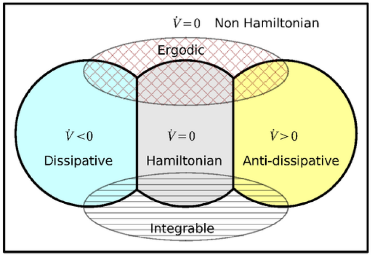
Figure 1: The set of all dynamical systems includes the dissipative ($\dot{V}<0$) and anti-dissipative ($\dot{V}>0$) system subsets. Their complement is the subset of volume conserving ($\dot{V}=0$) systems, in which the Hamiltonian systems are a subset. Integrable and ergodic systems are distinct subsets overlapping the previous subsets. Classical statistical physics is restricted to the ergodic subset, while deterministic physics is restricted to the integrable subset.

A general dynamical system is often defined by the phase space $\{\vec{z}\}$, a set of real vectors in a $N$-dimensional Euclidean space, generated by a set of first order ordinary differential equations

$$\dot{\vec{z}}=\vec{F}(\vec{z},t)\ .$$ (1)

The set of all dynamical systems is a too broad set to build thermodynamics upon. Dissipative systems have attractors, therefore their asymptotic behaviour is restricted to these attractors, which may be as simple as a single point in phases space. Richer attractors are limit cycles, and still richer attractors, the strange attractors, may have fractal dimension. Reversing time in a dissipative system produces an anti-dissipative system which tends asymptotically to explore the boundaries of the allowed phase space.

Naturally some systems may have some dissipative phase space coordinates and some other anti-dissipative coordinates. Among such systems the Hamiltonian systems form a special subset where the phase space variables may be chosen in conjugate pairs in such a way that each of them conserves its phase space area. The symplectic structure of phase space follows from the Hamiltonian $H(\vec{p},\vec{q})$ and the particular form of Hamilton’s equation of motion. Hamiltonian systems still form a too broad set for classical thermodynamics, since some of these systems have long range interactions for which energy is not scaling proportionally to volume or mass. Others Hamiltonian systems are fully integrable, that is decomposable into independent one-degree of freedom Hamiltonian systems (consisting each of one pair of conjugate variables). Due to the area conservation constraint, such systems cannot be chaotic.

However, for many Hamiltonian systems classical statistical mechanics can already be used without the assumption of extensivity, as discussed by Gross in this volume and elsewhere (e.g. Gross 2001), or Padmanabhan for gravitating systems (1990). This is the microcanonical description, which however still requires the ergodic hypothesis, which in turn requires a finite phase space volume. Further, physical systems are modelled over a finite time over which a statistical description makes sense. This often means that the strength of chaos, measured by the rate of exponential divergence of neighbouring trajectories, must be large enough to effectively provides an sufficiently good ergodic behaviour over the physically relevant finite time.

The Fermi-Pasta-Ulam (1955) oscillator model first showed that not any mechanical system is ergodic, and subsequent works on dynamical systems such as the Kolmogorov-Arnold-Moser (KAM) theorem provided many more indications that most dynamical systems are partly chaotic, or semi-ergodic. Thus typical Hamiltonian systems are in general not ergodic, therefore the ergodic hypothesis is not necessarily valid in integrable or semi-ergodic systems.

In integrable systems almost all the orbits are quasi-periodic, therefore the initial correlations given by the initial conditions are never erased. Although exactly integrable systems are exceptional, fully ergodic systems are also rare. Generic Hamiltonian systems possess phase space regions with local quasi-integrals, which are nevertheless riddled by a web of resonances and chaos. In such semi-ergodic systems the accessible phase space over finite but long “quasi-asymptotic” times can be confined to a subset of the non-integrable phase space that depends finely on the particular initial conditions. This leads to intermittent behaviours. In such systems the usual statistical mechanical tools are not appropriate to describe steady states, because sudden large fluctuations are possible after arbitrary long times.

In a mechanical description of a physical system the basic properties that imprint global symmetries are the invariant functions of the coordinates, the global integrals of motion. Since in all time independent mechanical systems the total energy function $E=H(\vec{p}(t),\vec{q}(t))$ is the associated invariant, it is not astonishing that energy plays a key role in thermodynamics. Any invariant of the system introduces a geometrical constraint in phase space that is obeyed by the system, despite the presence of many more remaining fully unconstrained degrees of freedom.

Here enters the crucial property that most systems where thermodynamics works sufficiently well must have: most of the degrees of freedom must be strongly chaotic, which means that beyond a relaxation time the unavoidable and not accountable perturbations of the rest of the Universe on the modelled system can no longer be neglected. Beyond this time a deterministic description of the system is impossible. If the perturbations are uncorrelated with the system degrees of freedom, then rapidly a strongly chaotic system will have an equal probability to visit almost all points of the non-integrable subspace of phase space. Therefore the ergodic principle in statistical mechanics only applies over the variables belonging to the sufficiently chaotic degrees of freedom. Then over these variables averaging works well. In contrast, each strict integral of motion lowers the dimension of the available phase space by one.

As an example of system with non-thermodynamical behaviour, for most initial conditions a gravitational 10-body system dissolves in a few crossing times, while for particular initial conditions like the present solar system ones the same 10-body system may stay bound over billions of crossing times. The solar system is therefore a prime case of semi-ergodic system on which classical thermodynamics does not apply. Over time-scale of a few million years only a small part of the degrees of freedom behave in a chaotic way (Laskar, 1994), indeed the other degrees of freedom are constraint not only by the 10 global classical integrals of motions, but also by additional local constraints that act almost like additional integrals of motion over very long finite time-scales.

A natural global quantity of a bounded mechanical Hamiltonian system following the orbit $\left\{\vec{P}(t),\vec{Q}(t)\right\}$ is the total visited phase space volume

$$\Gamma=\lim_{t\to\infty}{1\over 2t}\int_{-t}^{t}\!dt^{\prime}\int\!d^{N}\vec{q}\,d^{N}\vec{p}~{}\left[\delta\!\left(\vec{q}-\vec{Q}(t^{\prime})\right)\delta\!\left(\vec{p}-\vec{P}(t^{\prime})\right)\right]\ .$$ (2)

If the orbit were ergodic, almost all the points at constant value of $E$ of $H(\vec{p},\vec{q})$ would be included in $\Gamma$. This constant $E$ volume can also be expressed as

$$\Gamma_{E}=\int\!d^{N}\vec{q}\,d^{N}\vec{p}~{}\delta\!\left(E-H(\vec{p},\vec{q})\right)\ .$$ (3)

Every additional independent invariant function $I_{k}(\vec{p},\vec{q})$ restricts the available space space by one dimension in general systems, by two dimensions in Hamiltonian systems due to the symplectic constraint. If the number of chaotic degrees of freedom exceeds by far the number of invariant functions, the familiar situation for gases, the total accessible phase space volume remains a good approximation of the total phase space volume. This quantity, taken in the log, is, up to a constant, nothing else as Boltzmann’s original entropy $S=k_{B}\ln\Gamma_{H}$. For a statistical mechanics based on a well defined dynamics, such an entropy has a well defined sense. Without such a definition based on the particular system microdynamics, entropy remains a non-measurable quantity with obscure physical meaning.

Explicitely, if the Hamiltonian system has $N$ degrees of freedom, $M\leq N$ global independent integrals $I_{k}(p_{i},q_{i})$ with values $J_{k}$, and if the remaining accessible phase space is ergodic, then the log of the accessible volume,

$$\Gamma_{\rm ergodic}=\int\prod_{k=1}^{M̀}\delta\left(J_{k}-I_{k}(\vec{p},\vec{q})\right)\,dq_{i}^{N}dp_{i}^{N}\ ,$$ (4)

can be used as the system microcanonical entropy, on which a thermodynamics can be built.

1.4 Generalisations

From there it is straightforward to generalise these considerations for a wider class of dynamical systems. First, Hamiltonian systems form a subset of volume preserving systems. By taking a Cartesian product of simpler volume preserving systems and combining the variables by regular functions one can build more general coupled dynamical systems with an odd or even number of variables that are still volume preserving, and possess a number of global integrals of motion. Like for Hamiltonian systems the remaining accessible phase space however may or may not be effectively ergodic due to chaos. In the first case the entropy can be defined and be used to built upon a microcanonical thermodynamics.

For dissipative dynamical systems $\dot{\vec{z}}=\vec{F}(\vec{z})$ with orbit $\vec{Z}(t)$, the asymptotic attractors may still represent a non-trivial invariant subset of phase space which is eventually ergodic. For such systems the asymptotic thermodynamics is still a well defined procedure, just taken in the asymptotic limit of large time,

$$\Gamma_{\rm ergodic}=\lim_{t_{2}\to\infty}\lim_{t_{1}\to\infty}{1\over t_{2}}\int_{t_{1}}^{t_{1}+t_{2}}\!dt^{\prime}\int\!d\vec{z}~{}\delta\!\left(\vec{z}-\vec{Z}_{i}(t^{\prime})\right)\ .$$ (5)

Actually, most steady natural systems can be supposed to follow this route. Starting from non-equilibrium states they converge toward asymptotic average steady states due to dissipation, and are maintained on their respective final attractors by global integrals.

1.5 The reason for extensive variables

An important point to explicit is the reason why thermodynamical variables in the canonical description are supposed to be either intensive, i.e., position invariant, or extensive, i.e., scaling linearly with the spatial volume $V$. For some reason, rarely discussed in depth, the thermodynamical variable $X_{i}$ of a system with many degrees of freedom scales as

$$X_{i}\propto V^{\sigma}\ ,$$ (6)

where $\sigma=0$ or $\sigma=1$. To assume such scaling relations is a crucial step leading to the usual characteristics of classical thermodynamics. This symmetry allows to describe extensive systems with uniform prescriptions encouraging the belief that extensive thermodynamics is universally applicable.

Let us apply the considerations of previous section to explain why systems with a large number of degrees of freedom tend toward uniform density above some microscopic scale. The smooth average distribution of particles is necessary to describe macroscopic variables as differentiable, which is then required to allow the use of differential equations for describing globally out of equilibrium fluids only locally in thermal equilibrium. In such systems the particle Lagrangian $\mathcal{L}$ for the space coordinates $\{\vec{x}_{i}\}$ takes the usual form where $T$ is the kinetic energy and $U$ the potential energy,

$$\mathcal{L}=T(\dot{\vec{x}}_{i})-U({\vec{x}}_{i}),\quad i=1,\ldots N.$$ (7)

In systems where the particle interaction energy is negligible with respect to their kinetic energy, $|T|\gg|U|$. The Lagrangian becomes then independent on the space coordinate $\vec{x}_{i}$. Therefore any integral of the system and subs-system should adopt the same space and orientation invariance: the system of particles must tend toward a uniform spatial distribution of the particles. In velocity space the particles are constraint by a finite total energy, a spherical symmetry of the distribution function in velocity space with a finite second moment follows; for distinguishable particles the Maxwell-Boltzmann distribution follows. Therefore the uniform smooth mass density in classical gases and fluids in statistical equilibrium follows from the corresponding invariance of the Lagrangian and from the chaotic nature of motion of particles. The extensivity property follows then from the microscopic dynamical properties of chaotic particles subject to a mutual interaction energy small in regards of their kinetic energy. The intensive variables, for example the mass density $\rho$, derive from the ratio of two extensive variables, such as the ratio of the mass and the volume.

At this point it is clear that when the interaction potential energy is not negligible, at sufficiently low temperature, the rules of classical thermodynamics can break down. Indeed, as stressed for example by Lynden-Bell (1999), at sufficiently low temperature a phase transition occurs, the microcanonical specific heat becomes negative. The system is then thermally unstable, the homogeneity invariance breaks down due to coexisting phases.

At still lower temperature the interaction energy in the Lagrangian dominates; a crystal may form, in which case most of the degrees of freedom become frozen. The continuous translational invariance is then broken and replaced by a discrete lattice invariance. The remaining small motions of an ensemble of molecules around the lattice energy minima form again an extensive dynamical system which can be described with usual statistical physics at the condition that the small motions around the lattice minima are nevertheless chaotic, unlike the Fermi-Pasta-Ulam oscillators.

2 Non-extensive systems

However many cold systems with strong interaction potential do not develop regular lattices, among them glasses, or the gravitational $N$-body systems. Since the statistical behaviour of gravitational systems is observed to display similar properties across galaxies and the Universe, a statistical description of them can nevertheless be expected.

An important additional symmetry in systems of particles such as gravitational systems is that the long range interaction term is scale invariant. In other terms the potential energy follows the symmetry of $p$-homogeneous functions,

$$U(\lambda\vec{x}_{i})=\lambda^{p}U(\vec{x}_{i})\,,$$ (8)

where $\lambda$ is any real positive number, and $p$ is the power law exponent of the 2-particle potential; $p=-1$ for gravitational systems. For $p$ sufficiently negative the potential is short ranged, so we should expect to recover perfect gas behaviour at sufficiently negative $p$.

So if we follow the above reasoning, a system of strongly interacting particles might display statistical behaviour following different symmetries than the ones adopted in extensive systems: instead of spatial invariance, systems may be characterised by scale-invariant properties. A priori nothing obliges us to assume a smooth, differentiable average particle distributions. Distributions in the mathematical sense, such as fractal or statistically scale-invariant distributions are actually suggested by many physical systems, as popularised by Mandelbrot (1982). Such distributions are in general non-differentiable, but can still be represented by an ensemble of points, i.e., a superposition of Dirac distributions.

So the problem that we want to address is to describe statistically such systems without adopting the usual assumptions of thermodynamics, but using as much as possible the known constraints from the microdynamics. Clearly we do not want to start with the assumption of extensivity, but rather take the symmetries of the Lagrangian as a guide to describe it in a statistical way.

Instead of requiring microscopic extensivity which justifies smooth microscopic distributions just above the mean-free path scales, we want to allow instead scale-invariant hierarchical systems, since such systems appear frequently in nature. The consequence is that the usual mathematical tools mostly based on differential equations are no longer suited.

The main general statistical tool of particle dynamics is the virial theorem, which applies to any, smooth or non-smooth, distribution of particles. In the literature the virial theorem is often derived by averaging the fluid equations of motions. This approach assumes from the start that the distribution function is regular. However the more general route not requiring regularity is to use the Lagrange-Jacobi identity valid for any set of point mass particles.

The polar semi-moment of inertia $I$ about the origin of a system of particles of mass $m_{i}$

$$I={1\over 2}\sum_{i}m_{i}\vec{x}_{i}^{2}\,,$$ (9)

characterises the system average mass extension in space. Differentiating $I$ with respect to time, the acceleration of this global scalar quantity is seen to be linked to the system kinetic energy and the total moment of radial forces, where ${\vec{F}}_{i}=m_{i}\ddot{\vec{x}}_{i}$,

$$\ddot{I}=\sum_{i}m_{i}\dot{\vec{x}}_{i}^{2}+\sum_{i}{\vec{F}}_{i}\cdot{\vec{x}}_{i}\,.$$ (10)

If the forces derive from a sum of $p_{k}$-homogeneous potentials $U_{k}$,

$$\ddot{\vec{x}}=-\sum_{k}\nabla U_{k}({\vec{x}}_{i})\,,\qquad\textrm{where}\qquad U_{k}(\lambda\vec{x})=\lambda^{p_{k}}U_{k}(\vec{x})\,,$$ (11)

then the total moment of force is proportional to a sum of potential energies weighted with the homogeneity indexes $p_{k}$, thus

$$\ddot{I}=2T({\vec{x}}_{i}^{2})-\sum_{k}p_{k}U_{k}({\vec{x}}_{i})\,.$$ (12)

This is the Lagrange-Jacobi identity, slightly generalised with a sum of homogeneous potentials.

If the system is confined by a pressure at the boundary, this pressure has the same effect that a uniform negative kinetic energy distributed inside the system volume $V$. Since a non-relativistic kinetic pressure amounts to $2/3$ of the kinetic energy density, we can write in virial equilibrium ($\ddot{I}=0$) that

$$2T({\vec{x}}_{i}^{2})-\sum_{k}p_{k}U_{k}({\vec{x}}_{i})=3P_{\rm ext}V\,.$$ (13)

3 Hierarchical systems

1cm

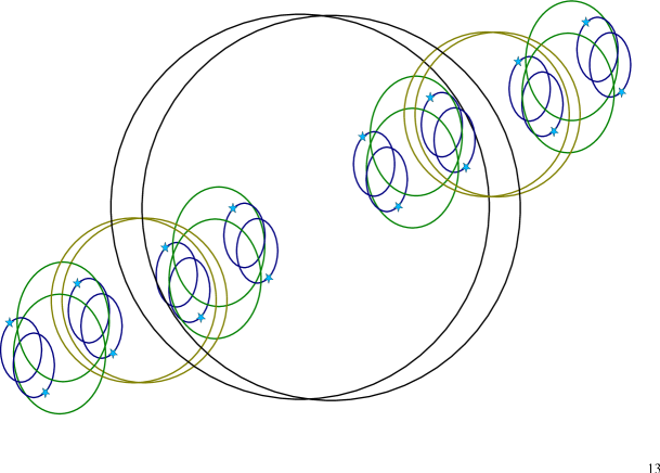
Figure 2: A hierarchical $2^{4}$-body system.

3.1 The hierarchical $N^{L}$-body problem

The gravitational $N$-body problem has played a central role in the development of classical mechanics and the theory of dynamical systems. It was seen for over 2 centuries as a prime example of the deterministic physics developed by Newton and followers. The main reason is, first, that the 2-body case is fully integrable, so computable over an arbitrary long time, and, second, that the planets move on orbits that are perturbations of the 2-body problem. Therefore the solar system remains well computable over centuries. But the works on the 3-body problem by Brun and Poincaré in the late 19^th century showed that the general $N$-body problem was of a different kind, not so easily computable. The notion of exponential divergence of nearby trajectories leading to the modern notion of chaos came then into existence.

Hierarchical $N$-body problems have been rarely studied (e.g., Nugeyre & Bouvier 1981). Yet such systems may provide others configurations than the planetary systems that are close to be integrable. Let us consider a bound 2-body gravitational system. If now we replace each body by an identical but scaled down 2-body problem at its centre of mass, and then recursively over a number $L$ of levels, then we have built a hierarchical $2^{L}$-body problem (Fig.2). This system is close to be integrable, since each 2-body subsystem is perturbed by the inner and the outer other 2-body systems. In order to avoid possible resonances we have the freedom to choose the scale ratio is such a way as to avoid rational ratios of orbital periods. Then in the limit of a large scale ratio the respective perturbations by the other bodies on each two body system is small, eventually negligible for at least the finite time we wish to consider such a system.

3.2 Geometrical relations

Let us first enumerate some simple but little known geometrical properties of mass particles arranged in a hierarchical way (Pfenniger & Combes 1994).

As first hypothesis we consider a system of mass $m_{L}$ made of $N$ clumps of mass $m_{L-1}$, made themselves of $N$ sub-clumps $m_{L-2}$, and so on over a number of levels. At any level $L>0$,

$$m_{L}=Nm_{L-1}\ .$$ (14)

In a regular hierarchical system the ratio of masses between adjacent levels is supposed to scale with spatial size according to a power law $d$,

$${m_{L}\over m_{L-1}}=\left({r_{L}\over r_{L-1}}\right)^{d}\ .$$ (15)

Since mass is positive, its cumulative value within a sphere centred on a mass point must monotonously increase with the sphere radius, so $d\geq 0$. In a 3-dimensional space, the positive cumulative mass cannot grow faster than volume, therefore $d\leq 3$.

As consequence there is a direct relationship between the adjacent level size ratio, $N$ and $d$,

$${r_{L}\over r_{L-1}}=N^{1/d}\ .$$ (16)

It follows straightforwardly that the average mass density scales as

$${\rho_{L}\over\rho_{L-1}}=\left({m_{L}/r_{L}^{3}\over m_{L-1}/r_{L-1}^{3}}\right)=\left({r_{L}\over r_{L-1}}\right)^{d-3}\ ,$$ (17)

which means that the average density increases at small scale for all permitted $d<3$.

In contrast, the projected mass density $\Sigma_{L}$ scales as

$${\Sigma_{L}\over\Sigma_{L-1}}=\left({m_{L}/r_{L}^{2}\over m_{L-1}/r_{L-1}^{2}}\right)=\left({r_{L}\over r_{L-1}}\right)^{d-2}\ .$$ (18)

Thus the critical exponent $d=2$ separates the projection of fractal objects of different $d$ (see also Falconer 1990). The immediate consequence for astronomical observations restricted by projected views of cosmic structures is that if a fractal object has $3\geq d>2$ then the sky is well filled by it, like common fog does. However, when $d<2$ most of the mass is projected in small spots, leaving most of the sky empty. Therefore a fractal distribution of galaxies with $d<2$ (Coleman & Pietronero 1992) is a possible (partial) explanation of the blackness of the Universe, the famous de Chéseaux-Olbers paradox.

3.3 Dynamical relations

Hierarchical distributions of gas are observed in the interstellar medium without a clear understanding of the overall physics. It seems clear that in a galaxy gravity plays a non-negligible role at most scales. Typically the interstellar gas fills the volume of a galaxy in a very inhomogeneous way well described by fractal geometry. The matter is fragmented in clumps themselves composed of sub-clumps over several order of magnitudes in scale. At each scale of a galaxy mass condensations are rather close to virial equilibrium from sizes comparable to the whole galaxy down to stars, passing by various interstellar clouds of intermediate sizes. Between the largest galaxy size and the smallest stellar size, a range of order $10^{12}$ is covered.

Generalising the gravitating case to other power law potentials, we adopt the potential form between mass particles,

$$\Phi(r)={GM\over p}\,r^{p}\ ,$$ (19)

with $p\neq 0$. The limit $p\to 0$ is well behaved and provides a logarithmic potential, that we do not discuss separately. For attracting interactions the coupling constant $G$ is positive. The gravitational case occurs for $p=-1$.

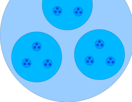
Figure 3: The mass hierarchical model over 4 levels with $N=3$.

Suggested by the system hierarchical organisation, we approximate the potential energy $U_{L}$ at level $L$ by retaining the first term of a multipolar expansion,

$$U_{L}=NU_{L-1}+\frac{G}{p}M_{L}^{2}r_{L}^{p}\left(1+\alpha\frac{r_{L-1}}{r_{L}}\right)\ .$$ (20)

The potential energy at a given level consists of the summed sub-clumps potential energies and the potential energy due to the interaction between the sub-clumps. The term containing $\alpha$ represents the first correction taking into account tidal interactions. Since the scale ratio is constant, the term in parentheses is constant and can be absorbed in a new coupling constant $G^{\prime}$. We will see that the main results do not depend on the value of $G$ (indeed scale invariance effects depend on the power law exponent $p$). For parameters suited to the interstellar medium ($D\approx 1-2$, $N=5-8$, Scalo 1990) the approximation (20) has been checked to be accurate at the percent level.

The third hypothesis is of statistical character. Thermodynamics can not be used since it excludes long-range interactions. The only remaining statistical tool is the virial theorem, more precisely the Lagrange-Jacobi indentity. If a scale invariant system finds a statistical equilibrium at each level, then the semi-moment of inertia acceleration $\ddot{I}$ of different sub-clumps vanishes in average, such that at each level,

$$2T_{L}-pU_{L}=3P_{L+1}V_{L}\,,$$ (21)

where $T_{L}$ is the total kinetic energy summed up level $L$, $P_{L+1}$ is the outer kinetic pressure, and $V_{L}\sim r_{L}^{3}$ the clump volume. Here the outer pressure is purely kinetic: it is given by $2/3$ of the kinetic energy density outside the sub-clumps. Approximately,

$$P_{L}=\frac{2}{3}{T_{L}-NT_{L-1}\over V_{L}-NV_{L-1}},$$ (22)

which takes into consideration that most of the time distinct clumps do not overlap.

3.4 Explicit solution

The above recurrences for $M_{L}$, $V_{L}$, $U_{L}$ and $T_{L}$ in Eqs. (14,15,20,21,22) can be solved with little algebra exactly in finite terms, as detailed below.

First we define a few convenient terms, and state simple constraints. The lowest level virial ratio,

$$\beta\equiv\frac{pU_{0}}{2T_{0}}$$ (23)

is obviously constraint from Eq. (21) divided by $2T_{L}$ in the interval $0\leq\beta\leq 1$, because $T_{L}$, $pU_{L}$, $V_{L}$, and $P_{L}$ are all positive. When $\beta\to 0$ the lowest level is confined by outer pressure, when $\beta\to 1$, by internal attraction.

The lowest level energy is $E_{0}=T_{0}+U_{0}$. The marginally bound state occurs when $E_{0}=0$. Such a state is possible only when

$$0<-p/2<1\,.$$ (24)

The scale ratios

$$x\equiv\frac{r_{L}}{r_{L-1}},\quad{\rm and}\quad X\equiv x^{L},$$ (25)

are by definition $>1$, since as shown in Eq. (16), $x=N^{1/d}>1$.

In terms of $x$ and $X$ we have,

$$\frac{m_{L}}{m_{0}}=X^{d},\quad{\rm and}\quad\frac{V_{L}}{V_{0}}=X^{3}.$$ (26)

It just means that the mass is proportional to the power $d$ of the size, while the volume to the power 3. Incidentally, the factor $X^{d-3}$ is the density ratio $\rho_{L}/\rho_{0}$.

Eq. (20) is a linear recurrence relation for $U_{L}$ that has a simple solution:

$$\frac{U_{L}/m_{L}}{U_{0}/m_{0}}=\frac{(Xx)^{d+p}-1}{x^{d+p}-1}\,,\qquad L\geq 0\,.$$ (27)

Some more effort is required to solve Eq. (21) by substitutions and induction. We obtain,

$$\frac{T_{L}/m_{L}}{T_{0}/m_{0}}=X^{3\!-\!d}+{\beta\over x^{d+p}\!-\!1}\left[{(Xx)^{3-\!d}\!-\!(Xx)^{d+\!p}\over x^{3-d}-x^{d+p}}+{X^{3-\!d}\!-\!X^{d+\!p}\over{1\over x^{3-d}}-{1\over x^{d+p}}}-1\right].$$ (28)

The equivalent of the kinetic pressure at each level is proportional to the square of the velocity dispersion $v_{L}$ given by,

$$\frac{1}{2}m_{L}v^{2}_{L} \equiv T_{L}\,,\qquad\qquad\quad L=0\,,$$ (29)

$$\equiv T_{L}-NT_{L-1}\,,\quad L\geq 1\,,$$ (30)

which means that the kinetic pressure is the difference between two adjacent levels of the summed kinetic energies down to the lowest level. Replacing with Eq.(28), we obtain,

$$\frac{v^{2}_{L}}{v^{2}_{0}}=\left(x^{3-d}-1\right)\bigg{[}\left(\frac{X}{x}\right)^{3-d}-\beta\frac{X^{3-d}-X^{d+p}}{x^{3-d}-x^{d+p}}\bigg{]}\,,\quad L\geq 1\,.$$ (31)

3.4.1 Physical domain of $p$ and $d$

The above hierarchical model makes sense in the intervals $0<d\leq 3$, for geometrical reason, and $p<0$ if we wish to consider interactions of attractive type not growing too fast with distance. As already understood by Newton, even the gravitating case $p=-1$ leads to conceptual problems when $d=3$ (the force at any point in a uniform infinite medium is a sum of cancelling diverging forces).

However, even in this restricted domain not any combination of $p$ and $d$ is physically feasible. One has to ensure that the positive quantities are indeed positive, and do not diverge to excessive values.

First one can easily check in Eq.[27] that $U_{L}/U_{0}$ does not change sign because $X>x>1$, and at $d+p=0$ the behaviour is regular.

The kinetic energy and the squared velocity (or the pressure) should remain positive and finite. In fact, by looking at Eq.[30] ones sees that it suffices to require the positivity of the squared velocity at each level to ensure that the summed kinetic energy is also positive.

A denominator vanishes in Eq.[28] when $d+p\to 0$. But more important, when $3-d\to d+p$ other denominators in Eqs.[28],[31] vanish with corresponding numerators containing cancelling powers of $X$. This latter singularity is crucial because it means that as the number of levels of the system increases, a shrinking domain of parameter space is able to correspond to accessible physical states. As shown in Fig.(4), on one side of the singularity $v^{2}_{L}$ is negative and on the other side it takes extremely large values, such that the only physical sensible region is within the singularity as $L\to\infty$.

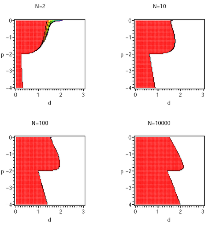
Figure 4: The ratio $v_{L}^{2}/v_{0}^{2}$, for $l=12$, in the plane $(d,p)$ takes either very large values exceeding $10^{4}$ in the shaded regions at low $d$, or negative values in the white region at large $d$, or physical values in the narrow intermediate region, for different $N$. In all cases the low level boundary condition is $\beta=\min(1,-p/2)$, which produces the discontinuity at $p=-2$.

Since $v^{2}_{L}$ can change its sign, we obtain a limit of physically admissible cases. Solving Eq.[31] for $\beta$ we obtain a constraint for $\beta$, noting $\alpha=(d+p)-(3-d)$,

$$v^{2}_{L}\geq 0\quad\Rightarrow\quad\beta\leq\frac{1-x^{\alpha}}{1-X^{\alpha}}.$$ (32)

Since $X>x>1$, the critical value $\beta_{\rm crit}$ is in the interval $(0-1)$ only when $\alpha>0$. To not be subject to this restriction on $\beta$, $d$ must obey

$$d\leq\min\left(3,{3-p\over 2}\right)\ .$$ (33)

For hierarchical gravitating systems with $d>2$, a range of $\beta<1$ is not allowed. At the lowest level an outer pressure is required.

3.5 Large $L$ limit

In ordinary systems the thermodynamical limit means that the boundary conditions, the “box”, takes an infinite dimension, $V\to\infty$ and $M\to\infty$, but $M/V\to\rm const<\infty$, or the number of particles $N$ tends toward infinity at constant average density. The mass and volume per particle are kept constant. In other cases, particularly relevant in gravitating systems such as stars in which local thermodynamics still works, the total mass and volume is taken as fixed, but the number of particles is increased to infinity by decreasing the mass $m$ and volume $v$ per particle to zero, keeping $m/v$ constant.

In hierarchical systems, one can also increase the number of particles, or degrees of freedom, toward infinity at either the large or small scales, by increasing the number of levels $L$. The boundary conditions, fixing typically the temperature in a box, can be replaced by the conditions at either small or large scale depending on the problem.

Here we take the analogue of a “thermodynamical limit” by $L\to\infty$, or $X=x^{L}\to\infty$. Then the shrinking of the range of physical solutions compatible with the virial theorem leads to the constraint,

$$d=\frac{3-p}{2-\frac{\ln(1-\beta)}{\ln N}}.$$ (34)

Equivalently, one can use

$$\beta=1-x^{\alpha}\,,\qquad\alpha=(d+p)-(3-d)\ .$$ (35)

For example for $p=-1$, $d<2$ in any case. For systems not too confined by the outer pressure ($1/2<\beta<1$) and $N>5$, we have $d<1.7$, while systems with more outer pressure (“pressure confined clouds”) increase $d$ up to 2. Therefore, we conclude that hierarchical gravitating systems in statistical equilibrium can indeed exist, but with $d<2$.

3.6 Velocity scaling

In the large $L$ limit, when using Eq.[35] the scale-velocity dispersion in Eq.[31] takes the exact scale-free form

$$\frac{v^{2}_{L}}{v^{2}_{0}}=\left(1-{1\over x^{3-d}}\right)X^{d+p}\,,\quad L\geq 1\,.$$ (36)

In other words

$$v\propto r^{\kappa}\,,\qquad\textrm{where}\qquad\kappa\equiv{d+p\over 2}\,.$$ (37)

For fractal ISM cold clouds with substantial ambient pressure, $\beta\approx 1/2$, and with $N=5-10$ (Scalo 1990), we expect $d\approx 1.7$ and $\kappa\approx 0.35$, which is compatible with Larson’s (1981) size-linewidth relationship.

4 Conclusions

Once one realises that despite its enormous success, classical statistical mechanics is not universal, but mostly applicable to extensive strongly chaotic systems, a huge field of investigations opens up. Classes of systems, including formal or non-physical systems, may eventually be found suited for a statistical description of their steady states provided their dynamics is sufficiently chaotic to allow the use of an ergodic hypothesis. However, many semi-ergodic systems exist with intermittent behaviour for which there is little motivation to expect that a statistical description of steady states is appropriate.

The non-extensive gravitational systems are the rule in astrophysics, and many observational evidences exist that suggest that gravitational systems may follow statistical rules. For example laws such as the $r^{1/4}$ radial density profile of elliptical galaxies, or the exponential profiles of stellar galactic disks are well known, and reproducible in computer simulations, but not fully explained by a statistical model.

Here as a illustrating example we have developed a statistical description of $N^{L}$ hierarchical systems subject to power law interaction without using concepts of classical statistical mechanics. Using the virial theorem instead one can already find new constraints that emerge for a large number of bodies. As application, Larson’s empirical velocity scaling relationship in molecular clouds is retrieved.

Acknowledgements

I thank the organisers for this stimulating, timely and useful meeting bridging different fields.

References

- Antonov (1962) Antonov, V.A. 1962, Bull. Leningrad. State Univ. N. 7, 135
- Coleman & Pietronero (1992) Coleman P.H., Pietronero L. 1992, Physics Reports 213, No 6
- Falconer (1990) Falconer K. 1990, Fractal Geometry, John Wiley & Sons, Chichester
- Fermi, Pasta & Ulam (1955) Fermi E., Pasta J., Ulam S. 1955, Los Alamos report LA-1940; 1965 in Collected Papers of Enrico Fermi, E. Segré (Ed.), Univ. of Chicago Press
- Hénon (1961) Hénon M. 1961, Annales d’Astrophysique, Vol. 24, p.369
- Gemmer et al. (2004) Gemmer J., Michel M., Mahler G. 2004, Quantum Thermodynamics, Emergence of Thermodynamic Behavior Within Composite Quantum Systems, Lecture Notes in Physics 657, Springer, Berlin
- Gross (2001) Gross D.H.E. 2001, Microcanonical thermodynamics: Phase transitions in “small” systems, Lecture Notes in Physics 66, World Scientific, Singapore 188
- Larson (1981) Larson R.B. 1981, Monthly Notices Royal Astron. Soc., 194, 809
- Laskar (1994) Laskar, J. 1994, Astron. Astrophys., 287, L9
- Lynden-Bell & Wood (1968) Lynden-Bell D., Wood R. 1968, Monthly Notices of the Royal Astronomical Society, 138, 495
- Lynden-Bell (1999) Lynden-Bell D., 1999, Physica A 263, 293–304
- Mandelbrot (1982) Mandelbrot. B, 1982, The Fractal Geometry of Nature, Freeman, New York
- Nugeyre & Bouvier (1981) Nugeyre, J. B. & Bouvier, P. 1981, Celestial Mechanics, 25, 51
- Padmanabhan (1990) Padmanabhan T. 1990, Statistical mechanics of gravitational systems, Physics Report 285, 188
- Pfenniger & Combes (1994) Pfenniger D., Combes F., 1994, Astron. Astrophys., 285, 94
- Scalo (1990) Scalo J., 1990, in Physical Processes in Fragmentation and Star Formation, R. Capuzzo-Dolcetta et al. (eds.), Kluwer, Dordrecht, 151
- Shannon (1948) Shannon, C.E. 1948, ”A Mathematical Theory of Communication”, Bell System Technical Journal, vol. 27, pp. 379-423, 623-656
- Tribus & Irvine (1971) Tribus M., Irvine E.C. 1971, Scientific American. September, 179