Motion of a vortex line near the boundary of a semi-infinite uniform condensate

Abstract

We consider the motion of a vortex in an asymptotically homogeneous condensate bounded by a solid wall where the wave function of the condensate vanishes. For a vortex parallel to the wall, the motion is essentially equivalent to that generated by an image vortex, but the depleted surface layer induces an effective shift in the position of the image compared to the case of a vortex pair in an otherwise uniform flow. Specifically, the velocity of the vortex can be approximated by $U\approx(\hbar/2m)\left(y_{0}-\sqrt{2}\xi\right)^{-1}$, where $y_{0}$ is the distance from the center of the vortex to the wall, $\xi$ is the healing length of the condensate and $m$ is the mass of the boson.

I. INTRODUCTION

Vortex dynamics in a Bose-Einstein condensate (BEC) has been studied intensively, initially in the context of superfluid helium and later in dilute trapped BECs. The motion of vortices in both uniform and inhomogeneous condensates has been the subject of many theoretical works, and extensive reviews of these efforts have been given in fetterRev ; pismen .

In this paper we consider the problem of vortex motion in an asymptotically homogeneous condensate in the presence of a solid wall where the wave function of the condensate vanishes. Recent discussions (see, for example, anglin and references therein) on the motion of vortices near the surface of trapped condensates have questioned the relevance of the method of images in describing this motion. In that case, the nonuniform condensate density is approximated by a linear function that vanishes at the Thomas-Fermi surface, and the vortex motion can be considered to arise principally from the local density gradient. Here, we consider a rather different situation, in which the condensate density approaches its bulk value within a healing length $\xi$, and the vortex is located in the asymptotically uniform region. In this latter case, the local gradient of the condensate density is very small. The motion can be interpreted as arising from an image, but the depleted surface layer induces an effective shift in the position of the image in comparison with the case of a uniform incompressible fluid.

Our geometry is two dimensional, with the vortex aligned along the $z$ axis, parallel to the surface of the wall. The dynamics of the time-dependent BEC in the presence of the solid wall at $y=0$ is described by the Gross-Pitaevskii (GP) equation

$$-2{\rm i}\psi_{t}=\nabla^{2}\psi+(1-|\psi|^{2})\psi,$$ (1)

subject to the boundary conditions

$$\psi(x,y=0,t)=0,\qquad 0\leq y<\infty,\quad|x|<\infty,$$ (2)

in dimensionless units, such that the distance is measured in healing lengths $\xi=\hbar/\sqrt{2mgn_{0}}$, where $g$ is a two-dimensional coupling constant with dimension of energy times area, $m$ is the mass of the boson and $n_{0}$ is the bulk number density per unit area. Time is measured in units of $m\xi^{2}/\hbar$ and energy in units of $\hbar^{2}n_{0}/m$. In our units, the speed of sound $c$ in the bulk condensate is $c=1/\sqrt{2}$.

In the absence of vortices, the exact solution of (1) for the stationary state of the semi-infinite condensate is

$$f(y)=\tanh(y/\sqrt{2}).$$ (3)

In classical inviscid fluid dynamics with constant mass density $\rho$, the relevant kinematic boundary condition at a solid wall with normal vector ${\bf n}$ is

$$\rho\,{\bf u}\cdot{\bf n}=0,$$ (4)

where $\bf u$ is the velocity of the fluid. The corresponding problem of a vortex moving parallel to the wall is solved by placing one or more image vortices in such a way that condition (4) is identically satisfied.

For the dynamics described by the GP equation (1), the density $\rho\propto|\psi|^{2}$ is no longer constant, but rather vanishes at the surface of the wall. Thus condition (4) is automatically satisfied, and all components of ${\bf u}$ can in principle remain finite on the boundary. Therefore, it may seem that image vortices are irrelevant in the case of the GP equation, so that the vortex should remain stationary away from the boundary (where the fluid density is constant apart from exponentially small corrections). Our numerical simulations show that this is not true. In fact, the vortex moves parallel to the boundary, and it moves faster than a corresponding pair of vortices of opposite circulation in a uniform condensate in the absence of the depletion caused by the boundary. The purpose of our paper is to study this motion in detail.

The paper is organized as follows. In Sec. II we find the family of disturbances moving with a constant velocity along the solid wall by numerically solving the Gross-Pitaevskii (GP) equation in the frame of reference moving with the disturbance. In Sec. III a time-dependent Lagrangian variational analysis is used to find the first two leading terms in the equation of the vortex motion in the limit of large distance from the wall. In Sec. IV an alternative approach based on the dependence of total energy and momentum on the vortex position is used to determine the vortex velocity. In Sec. V we summarize our main findings.

II. Numerical solutions

In what follows we seek solitary-wave solutions of Eq. (1) that preserve their form as they move parallel to the wall with fixed velocity $U$. For each value of the velocity $U$, we have

$$\psi(x,y,t)=\psi(\eta,y),$$

where $\eta=x-Ut$. The GP equation (1) becomes

$$2{\rm i}U\psi_{x}=\nabla^{2}\psi+(1-|\psi|^{2})\psi,$$ (5)

where we set $x=\eta$. In the absence of the wall, the solitary-wave solutions of Eq. (5) were found by Jones and Roberts jr4 . For each value of $U$, there is a well-defined momentum $p$ and energy $E$, given by

$$p = \textstyle{\frac{1}{2{\rm i}}}\int\left[(\psi^{*}-1)\partial_{x}\psi-(\psi-1)\partial_{x}\psi^{*}\right]\,dxdy\,,$$ (6)

$$E = {\textstyle{\frac{1}{2}}}\int|\bm{\nabla}\psi|^{2}\,dxdy\ +\ {\textstyle{\frac{1}{4}}}\int(1-|\psi|^{2})^{2}dxdy\,.$$ (7)

In a momentum-energy $pE$ plot, the family of such solitary-wave solutions consists of a single branch that terminates at $p=0$ and $E=0$ as $U\rightarrow c$ (we call this curve the “JR dispersion curve”). For small $U$ and large $p$ and $E$, the solutions are asymptotic to pairs of vortices of opposite circulation. As $p$ and $E$ decrease from infinity, the solutions begin to lose their similarity to vortex pairs. Eventually, for a velocity $U\approx 0.43$ (momentum $p_{0}\approx 7.7$ and energy $E_{0}\approx 13.0$) they lose their vorticity ($\psi$ loses its zero), and thereafter the solutions may better be described as “rarefaction waves” that can be thought of as finite amplitude sound waves. The velocity of the vortex pair in the absence of the boundary is plotted as a function of the position of the vortices $\pm y_{0}$ shown in Fig. 1. The dashed line gives the asymptotic velocity valid for large $y_{0}$ as $U=(2y_{0})^{-1}$.

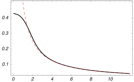
Figure 1: [Color online] Graphs of the velocity of the vortex $U$ versus the vortex position $y_{0}$ as calculated via numerical integration of (5) subject to the boundary conditions $\psi\rightarrow 1$ as $x^{2}+y^{2}\rightarrow\infty$ without the wall (solid line) and the asymptotics given by $U=(2y_{0})^{-1}$ (dashed line).

In analogy with these results, we used numerical methods to find the complete family of solitary-wave solutions of (5) subject to the hard-wall boundary condition (2). Specifically, we mapped the semi-infinite domain onto the box $(-\frac{\pi}{2},\frac{\pi}{2})\times(0,\frac{\pi}{2})$ using the transformation $\widehat{x}=\tan^{-1}(Dx)$ and $\widehat{y}=\tan^{-1}(Dy),$ where $D\sim 0.4-1.5$. The transformed equations were expressed in a second-order finite-difference form using $200^{2}$ grid points, and the resulting nonlinear equations were solved by the Newton-Raphson iteration procedure, using a banded matrix linear solver based on the bi-conjugate gradient stabilised iterative method with preconditioning. Similar to jr4 , we are interested in finding the dispersion curve for our solutions in the $pE$ plane. The energy and impulse of each solitary wave are defined by the expressions (6)-(7) appropriately modified for the “ground state” given by $f(y)$:

$$p = \textstyle{\frac{1}{2{\rm i}}}\int\left[(\psi^{*}-f(y))\partial_{x}\psi-(\psi-f(y))\partial_{x}\psi^{*}\right]\,dxdy\,,$$ (8)

$$E = \textstyle{{\frac{1}{2}}}\int\left[|\bm{\nabla}\psi|^{2}\ +\textstyle{{\frac{1}{2}}}(1-|\psi|^{2})^{2}-{\rm sech}^{4}(y/\sqrt{2})\right]\,dxdy\,.$$ (9)

In Fig.  2, we show the resulting solutions in the $pE$ plane. The plot of the velocity dependence on the vortex position is given below in Fig. 3 in Sec. IV. All our vortex solutions with a rigid wall (those with a node in the fluid’s interior) move with velocities less than $U=0.47$. For $U>0.47$, the zero of the wave function occurs on the wall only, and the solitary waves resemble rarefaction pulses of the JR dispersion curve away from the wall.

Figure 2: [Color online] The momentum-energy curve of the solitary wave solutions of Eq. (5) with the solid wall (solid line) and the JR dispersion curve (dashed line) that has no solid wall. For the solid-wall boundary condition, the vortex solutions with nonzero vorticity and nodes are shown in black and the vorticity-free solutions in grey (green).

III. Variational approach

The time-dependent variational Lagrangian method offers a convenient analytical approach to estimate the vortex velocity for large $y_{0}$. The dimensionless GP equation is the Euler-Lagrange equation for the time-dependent Lagrangian functional

$${\cal L}={\cal T}-{\cal E}\equiv\textstyle{\frac{1}{2}}{\rm i}\int\left(\psi^{*}\psi_{t}-\psi_{t}^{*}\psi\right)dxdy-\textstyle{\frac{1}{2}}\int\left(|\bm{\nabla}\psi|^{2}+\textstyle{\frac{1}{2}}|\psi|^{4}\right)dxdy$$ (10)

where the time-dependent terms constititute the “kinetic energy” $\cal T$ and the remaining terms are the GP energy functional $\cal E$.

We assume a trial function that depends on one or more parameters, and use this trial function to evaluate the Lagrangian $\cal L$ in Eq. (10), which will depend on the parameters and their first time derivatives. The resulting Euler-Lagrange equations determine the dynamical evolution of the parameters. For the present problem of a vortex moving parallel to a rigid boundary with the boundary condition (2), the vortex coordinates ($x_{0},y_{0}$) serve as the appropriate parameters, where $-\infty<x_{0}<\infty$ and $0<y_{0}<\infty$.

When the condensate contains a vortex at a distance $y_{0}$ from the boundary, the original condensate wave function (3) acquires both a phase $S({\bf r,\bf r}_{0})$ and a modulation near the center of the vortex, where the density vanishes. To model this behavior for the half space, it is preferable to include an image vortex at the image position $(x_{0},-y_{0})$. In this case, the approximate variational contribution to the phase is

$$S({\bf r},{\bf r}_{0})=\arctan\left(\frac{y-y_{0}}{x-x_{0}}\right)-\arctan\left(\frac{y+y_{0}}{x-x_{0}}\right),$$ (11)

where the second term reflects the negative image vortex. The derivation of the Gross-Pitaevskii equation involves an integration by parts of the kinetic energy density $|\bm{\nabla}\psi|^{2}$ to yield $-\psi^{*}\nabla^{2}\psi$ plus a surface term proportional to $\psi^{*}\partial_{y}\psi$ and this is one rationale for including the image. Strictly speaking, this term vanishes because $f(0)$ does so, but the image vortex ensures that the contribution vanishes even in the case of a uniform condensate. The image vortex also cuts off the long-range tail of the velocity, giving a convergent kinetic energy even for a semi-infinite condensate. It thus seems more physical to include the image in this particular geometry, even though the image is often omitted for the highly nonuniform density obtained in the Thomas-Fermi limit for a trapped condensate anglin ; al ; Kim04 ; Kim05 .

In addition, the vortex affects the density near its core, which is modeled by a factor $v(|{\bf r}-{\bf r}_{0}|)$, where $v(r)$ vanishes linearly for small $r=\sqrt{x^{2}+y^{2}}$ and $v(r)\to 1$ for $r\gg 1$ fe68 ; al . In principle, the function $v(r)$ can be taken as the exact radial solution of the Gross-Pitaevskii equation in an unbounded condensate, but this choice requires numerical analysis, and it is often preferable to use a variational approximation. A particularly simple choice is Fisc03

$$v(r)=\begin{cases}r/\lambda&\text{for $r\leq\lambda$};\\ 1&\text{for $r\geq\lambda$},\par\end{cases}$$ (12)

where $\lambda$ is the effective vortex core size; a variational analysis yields the optimal value $\lambda=\sqrt{6}$. With these various approximations, the variational trial function is al

$$\psi({\bf r},{\bf r}_{0},t)=\,e^{iS({\bf r},{\bf r}_{0})}\,f(y)\,v(|({\bf r}-{\bf r}_{0}|).$$ (13)

The time-dependent part of the functional in Eq. (10) becomes

$${\cal T} = -\displaystyle{\int\left[f(y)\right]^{2}\partial_{t}S\,\left|v(|{\bf r}-{\bf r}_{0}|)\right|^{2}}\,dxdy\approx-\int\left[f(y)\right]^{2}\partial_{t}S\,dxdy,$$ (14)

where the last approximation omits the effect of the vortex on the density, replacing $|v|^{2}$ by 1 throughout the condensate. A straightforward analysis then yields

$${\cal T}\approx 2\pi\,\dot{x}_{0}\int_{0}^{y_{0}}\left[f(y)\right]^{2}\,dy,$$ (15)

where $\dot{x}_{0}$ is the velocity $U$ of the vortex parallel to the wall.

The contribution to $\cal T$ from the vortex core yields a term that is smaller than Eq. (15) by a factor of relative order $y_{0}^{-2}$, which is negligible relative to the leading correction of order $y_{0}^{-1}$ that we retain here.

Since the energy functional will turn out to depend only on the single coordinate $y_{0}$, the Euler-Lagrange equation for $x_{0}$ implies that $y_{0}$ remains constant (as expected from energy considerations). In contrast, the equation for $y_{0}$ reduces to

$$\frac{d}{dt}\,\frac{\partial{\cal L}}{\partial\dot{y}_{0}}=\frac{\partial{\cal L}}{\partial y_{0}}=0,$$ (16)

since $\dot{y}_{0}$ does not appear in ${\cal T}$ (and hence in $\cal L$). Thus the dynamical motion of the vortex is given by

$$\dot{x}_{0}\approx\frac{1}{2\pi\left[f(y_{0})\right]^{2}}\,\frac{\partial{\cal E}}{\partial y_{0}}.$$ (17)

It is evident that only the derivative $\partial{\cal E}/\partial y_{0}$ is relevant, so that several terms in $\cal E$ play no role in the present analysis. For example, the derivative of the interaction energy ${\cal E}_{\rm int}(y_{0})=\frac{1}{4}\int|\psi|^{4}\,dxdy$ vanishes exponentially for $y_{0}\gg 1$ and does not affect the dynamics of the vortex for large $y_{0}$. Similarly, the kinetic energy in Eq. (10) separates into two parts, arising from the density variation and the flow energy, respectively; the contribution from the density variation is also negligible for $y_{0}\gg 1$.

The remaining (dominant) kinetic energy ${\cal E}_{kv}=\frac{1}{2}\int|\bm{\nabla}S|^{2}\,|\psi|^{2}\,dxdy$, arises from the vortex flow. The squared velocity now follows from Eq. (11)

$$|\bm{\nabla}S|^{2}=\frac{y_{0}}{y}\left[\frac{1}{(x-x_{0})^{2}+(y-y_{0})^{2}}-\frac{1}{(x-x_{0})^{2}+(y+y_{0})^{2}}\right].$$ (18)

The resulting flow-induced kinetic energy is

$${\cal E}_{kv}=\frac{1}{2}\int f(y)^{2}\,v(|{\bf r-\bf r}_{0}|)^{2}\,|\bm{\nabla}S|^{2}\,dxdy.$$ (19)

It is convenient to divide this integral up into three (strip-shaped) regions

$$\text{region I}: 0\leq y\leq y_{0}-\lambda v=1$$ (note that in I) (20)

$$\text{region II}: y_{0}-\lambda\leq y\leq y_{0}+\lambda$$ (21)

$$\text{region III}: y_{0}+\lambda\leq y\leq\infty v=1$$ (note that in III) (22)

In region II, inside the vortex core $|{\bf r-\bf r}_{0}|\leq\lambda$, the integrals can be found approximately in cylindrical coordinates and yield ${\cal E}_{kvc}\approx(\pi/2)f(y_{0})^{2},$ neglecting terms of order $\lambda^{2}/y_{0}^{2}$. The remaining region of the strip II outside the core simplifies because $v=1$. It is convenient to parametrize $y=y_{0}+\lambda\sin\theta$ by an angle $\theta$ that runs from $-\pi/2$ to $\pi/2$. In this region, the symmetry in $x$ allows us to consider only $x\geq 0$, and the lower limit for $x$ is $x_{m}(\theta)=\lambda\cos\theta$. The relevant integral is

$${\displaystyle\int_{x_{m}(\theta)}^{\infty}\left[\frac{1}{x^{2}+(y-y_{0})^{2}}-\frac{1}{x^{2}+(y+y_{0})^{2}}\right]}\,dx$$ (23)

$$\qquad= {\displaystyle\frac{1}{|y-y_{0}|}\left[\frac{\pi}{2}-\arctan\left(\frac{x_{m}(\theta)}{|y-y_{0}|}\right)\right]-\frac{1}{y+y_{0}}\left[\frac{\pi}{2}-\arctan\left(\frac{x_{m}(\theta)}{y+y_{0}}\right)\right]}$$

$$\qquad\approx {\displaystyle\frac{|\theta|}{\lambda|\sin\theta|}-\frac{\pi}{4y_{0}}}.$$

The total answer for region II is

$${\cal E}_{kv\rm II}\approx\pi f(y_{0})^{2}\left[\frac{1}{2}+\ln 2-\frac{\lambda}{2y_{0}}+\cdots\right],$$ (24)

where $\ln 2$ arises from the definite integral $\int_{-\pi/2}^{\pi/2}|\theta|/|\tan\theta|\,d\theta=\pi\ln 2$.

In regions I and III, the integrals can be found in cartesian coordinates, integrating over $x$ first. Each of these gives two contributions; one is simply a combination of logarithms obtained by replacing $f^{2}$ by $1$ and the other from the remainder with $-(1-f^{2})=-{\rm sech}^{2}(y/\sqrt{2})$.

$${\cal E}_{kv\rm I} = \frac{\pi}{2}\,\ln\left(\frac{2y_{0}-\lambda}{\lambda}\right)-\frac{\pi}{2}\int_{0}^{y_{0}-\lambda}{\rm sech}^{2}(y/\sqrt{2})\,\left(\frac{1}{y_{0}-y}+\frac{1}{y_{0}+y}\right)\,dy$$ (25)

$${\cal E}_{kv\rm III} = \frac{\pi}{2}\,\left[2\ln\left(\frac{y_{0}+\lambda}{\lambda}\right)-\ln\left(\frac{2y_{0}+\lambda}{\lambda}\right)\right]$$ (26)

$$-\frac{\pi}{2}\int_{y_{0}+\lambda}^{\infty}{\rm sech}^{2}(y/\sqrt{2})\,\left(\frac{1}{y-y_{0}}+\frac{1}{y+y_{0}}-\frac{2}{y}\right)\,dy.$$

To evaluate $\partial{\cal E}_{kv\rm I}/\partial y_{0}$ and $\partial{\cal E}_{kv\rm III}/\partial y_{0}$, we first differentiate the expressions in Eqs. (25) and (26), expand the integrands in the powers of $1/y_{0}$ through $O(y_{0}^{-2})$ and integrate to get

$$\frac{\partial{\cal E}_{kv\rm I}}{\partial y_{0}} \approx \frac{\pi}{2y_{0}-\lambda}+\frac{\sqrt{2}\pi}{y_{0}^{2}}{\rm tanh}\left(\frac{y_{0}-\lambda}{\sqrt{2}}\right),$$ (27)

$$\frac{\partial{\cal E}_{kv\rm III}}{\partial y_{0}} \approx \frac{\pi y_{0}}{(\lambda+y_{0})(\lambda+2y_{0})}.$$ (28)

A combination of these contributions gives the vortex velocity in Eq. (17) as

$$U=\dot{x}_{0} \approx \frac{1}{2}{\rm coth}^{2}\frac{y_{0}}{\sqrt{2}}\biggl{[}\frac{1}{2y_{0}-\lambda}+\frac{y_{0}}{(y_{0}+\lambda)(2y_{0}+\lambda)}$$ (29)

$$+ \sqrt{2}\biggl{(}\frac{1}{2}-\frac{\lambda}{2y_{0}}+\ln 2\biggr{)}{\rm sech}^{2}\bigl{(}\frac{y_{0}}{\sqrt{2}}\bigr{)}{\rm tanh}\bigl{(}\frac{y_{0}}{\sqrt{2}}\bigr{)}$$

$$+ \frac{\lambda}{2y_{0}^{2}}\,{\rm tanh}^{2}\left(\frac{y_{0}}{\sqrt{2}}\right)+\frac{\sqrt{2}}{y_{0}^{2}}\,{\rm tanh}\left(\frac{y_{0}-\lambda}{\sqrt{2}}\right)\biggr{]}.$$

This further simplifies to

$$U\approx\frac{1}{2}\biggl{(}\frac{1}{2y_{0}-\lambda}+\frac{y_{0}}{(y_{0}+\lambda)(2y_{0}+\lambda)}+\frac{\lambda+2\sqrt{2}}{2y_{0}^{2}}\biggr{)},$$ (30)

after we approximate the hyperbolic functions by their large $y_{0}$ behavior. When we neglect terms of order $1/y_{0}^{3}$, the expression (30) finally reduces to

$$U\approx\frac{1}{2y_{0}}\biggl{(}1+\frac{\sqrt{2}}{y_{0}}\biggr{)},$$ (31)

independent of $\lambda$.

IV. Vortex velocity through the Hamiltonian relationship between energy and impulse

In this section we present a different approach to the asymptotics for the vortex velocity based on the relationship between energy and momentum of the vortex pair. We compare the motion of a pair of vortices of opposite circulation (JR solutions) that satisfy

$$2iU_{1}\psi_{1x}=\nabla^{2}\psi_{1}+(1-|\psi_{1}|^{2})\psi_{2},\qquad|\psi_{1}|\rightarrow 1\qquad|{\bf x}|\rightarrow\infty,$$ (32)

with the motion of a vortex next to the solid wall

$$2iU_{2}\psi_{2x}=\nabla^{2}\psi_{2}+(1-|\psi_{2}|^{2})\psi_{2},\qquad|\psi_{2}|\rightarrow|\tanh(y/\sqrt{2})|\qquad|{\bf x}|\rightarrow\infty.$$ (33)

For the asymptotics, we are interested in the solutions for small $U_{i}$, for $i=1,2$, that correspond to a pair of vortices of opposite circulation. We calculate the following quantities: the position of the pair $(0,\pm y_{0})$, the energy and impulse given by (7)-(6) for $i=1$ and by (9)-(8) for $i=2$, so that

$$U_{i}=\frac{\partial E_{i}}{\partial p_{i}}.$$ (34)

These expressions for $i=1$ were derived in jr4 ; jr5 ; similar arguments immediately lead to the expressions for $i=2$.

Note that $U_{i},E_{i}$ and $p_{i}$ are functions of $y_{0}$ and if $y_{0}\gg 1$,

$$E_{1}=2\pi\log(2y_{0}),\qquad p_{1}=4\pi y_{0},$$ (35)

(see, for instance, pitaevskii ). From (34) we have

$$U_{1}=\frac{\partial E_{1}/\partial y_{0}}{\partial p_{1}/\partial y_{0}}=\frac{1}{2y_{0}},$$ (36)

as expected.

For large $y_{0}$ an accurate approximation to the solution of (32) for the uniform flow was found b04 as $\psi_{1}=u_{1}(x,y)+iv_{1}(x,y)$ where

$$u_{1}(x,y) = (x^{2}+y^{2}-y_{0}^{2})\tilde{R}(\sqrt{x^{2}+(y-y_{0})^{2}})\tilde{R}(\sqrt{x^{2}+(y+y_{0})^{2}}),$$

$$v_{1}(x,y) = -2xy_{0}\tilde{R}(\sqrt{x^{2}+(y-y_{0})^{2}})\tilde{R}(\sqrt{x^{2}+(y+y_{0})^{2}}),$$ (37)

where $\tilde{R}(r)=\sqrt{(0.3437+0.0286r^{2})/(1+0.3333r^{2}+0.0286r^{4})}.$ Another accurate choice is $\tilde{R}(r)=(r^{2}+2)^{-1/2}$. Similarly, we expect that $\psi_{2}$ is accurately approximated by $\psi_{2}=\psi_{1}|\tanh(y/\sqrt{2})|$.

The question we pose is: What is the position of the vortex $(0,y_{0})$ moving parallel to the solid wall with the same velocity as the vortex pair at $(0,y_{0}-l)$ in the uniform flow? Thus we seek the solution of

$$U_{1}(y_{0}-l(y_{0}))=U_{2}(y_{0})=\frac{\partial E_{2}/\partial y_{0}}{\partial p_{2}/\partial y_{0}},$$ (38)

where we explicitly indicate the dependence of $U_{1}$ and $U_{2}$ on the vortex position. Since $U_{1}(y_{0}-l)=(2(y_{0}-l))^{-1}$, we obtain the expression for the shift in the vortex position, $l$, in the presence of the wall as

$$l(y_{0})=y_{0}-\frac{1}{2}\frac{\partial p_{2}/\partial y_{0}}{\partial E_{2}/\partial y_{0}}.$$ (39)

We rearrange the right-hand side of (39) and use (35) to obtain the final equation that determines $l(y_{0})$:

$$l(y_{0})=y_{0}-\frac{1}{2}\frac{4\pi+\widetilde{dp}}{2\pi/y_{0}+\widetilde{dE}},$$ (40)

where $\widetilde{dE}=\partial(E_{2}-E_{1})/\partial y_{0}$ and $\widetilde{dp}=\partial(p_{2}-p_{1})/\partial y_{0}$ in the integral form given by (7)-(6) for $E_{1}$ and $p_{1}$ and (9)-(8) for $E_{2}$ and $p_{2}$. In evaluating the contribution $E_{2}-E_{1}$ only the kinetic terms involving derivatives with respect to $x$ were kept. The integrals $\widetilde{dE}$ and $\widetilde{dp}$ are exactly integrable in $x$ with the use of Mathematica, in which the leading order terms in $1/y_{0}$ are given by

$$\widetilde{dp} = -\frac{8\pi}{y_{0}^{3}}\int_{-\infty}^{\infty}{\rm sech}^{2}(y/\sqrt{2})\,dy+O(y_{0}^{-5}),$$

$$\widetilde{dE} = \biggl{(}\frac{\pi}{y_{0}^{2}}+\frac{\pi(\pi^{2}-18)}{2y_{0}^{4}}\biggr{)}\int_{-\infty}^{\infty}{\rm sech}^{2}(y/\sqrt{2})\,dy+O(y_{0}^{-6}).$$ (41)

With $\int_{-\infty}^{\infty}{\rm sech}^{2}(y/\sqrt{2})\,dy=2\sqrt{2}$ we finally arrive at

$$l(y_{0})=\frac{\sqrt{2}y_{0}(\pi^{2}+2(y_{0}^{2}-5))}{\sqrt{2}\pi^{2}+2(y_{0}^{3}+\sqrt{2}y_{0}^{2}-9\sqrt{2})}=\sqrt{2}+O(y_{0}^{-1}).$$ (42)

The vortex next to the wall moves with the velocity

$$U_{2}=\frac{1}{2(y_{0}-\sqrt{2})},$$ (43)

which is the main result of our asymptotics. Note that if we expand (43) in a Taylor series we get $U_{2}=\left(2y_{0}\right)^{-1}\left(1+\sqrt{2}/y_{0}\right)$, which agrees with the result of Section III. Fig. 3 gives the plot of the vortex velocity $U$ as a function of the distance of the vortex from the wall $y_{0}$ for the numerical solutions found in Sec. II, asymptotics found in Sec. III [see Eq.(31)] and asymptotics (43).

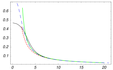
Figure 3: [Color online] Graphs of the vortex velocity $U$ versus its distance from the wall $y_{0}$ as calculated via numerical integration of (33) (black solid line) and the asymptotics given by (31) (red short-dashed line) and by (43) (green solid line). Also shown is the velocity of the vortex calculated by numerically integrating the right-hand side of (38) (blue long-dashed line). As one can see the simplifications made to derive (43) are consistent with the full expression (38) for $y_{0}>4$.

V. Discussion and Conclusions

In a uniform superfluid with a solid boundary, the motion of a quantized vortex arises from the image that enforces the condition of zero normal flow at the wall. In a trapped condensate, however, the image is generally omitted. Instead, the motion can be considered to arise from the gradient of the trap potential, which is the same as the gradient in the density in the Thomas-Fermi limit fetterRev . This behavior is especially clear for a single vortex at a distance $r_{0}$ from the center of a cylindrical container of radius $R$ Kim04 . For a classical incompressible fluid, the vortex precesses at an angular velocity

$$\left.\dot{\phi}\right|_{\rm cl}=\frac{\hbar}{m}\,\frac{1}{R^{2}-r_{0}^{2}}$$ (44)

because of the image vortex at $R^{2}/r_{0}$. In contrast, the precession rate in a trapped cylindrical condensate in the Thomas-Fermi limit

$$\left.\dot{\phi}\right|_{\rm TF}\approx\frac{\hbar}{m}\,\frac{\ln(R/\xi)}{R^{2}-r_{0}^{2}}$$ (45)

is larger than (44) because of the (typically large) logarithmic factor. Although the denominators of (44) and (45) both vary quadratically with $r_{0}$, the first result arises from the image and the second from the parabolic trap potential (and thus the parabolic density). If an image were included in the analysis of the trap, it would add a correction of order 1 to the large logarithm $\ln(R/\xi)$; such a term is comparable to other terms that are usually omitted.

As an intermediate situation between these two extremes, the present paper has analysed the dynamics of a vortex in a half space bounded by a solid wall on which the density of condensate vanishes. This geometry represents the simplest problem of a vortex in a condensate interacting with a surface. Since the gradient of the density vanishes exponentially for $y_{0}\gg\xi$, only the image remains to drive the motion in the asymptotic region. Our geometry allows us to separate the effect of the surface from the effect of the density gradient, both of which appear in the more complicated problem of an inhomogeneous trapped condensate anglin . We found the complete family of solitary-wave solutions moving with subcritical velocities parallel to the wall. In addition, both a variational analysis and the Hamiltonian relationship between energy and momentum were used to give the velocity of the vortex as a function of its distance from the wall. These results are identical through to the first correction term, where the small parameter is the inverse distance from the wall. Our main results are (i) that the vortex moves as if there was an image vortex on the other side of the wall, which essentially replaces the boundary condition (4) with a more stringent requirement ${\bf u}\cdot{\bf n}=0$ and (ii) that the depleted surface layer induces an effective shift in the position of the image in comparison with the case of the uniform flow. Specifically, the velocity of the vortex can be approximated by

$$U\approx\frac{\hbar}{2m(y_{0}-\sqrt{2}\xi)},$$ (46)

where $y_{0}$ is the distance from the center of the vortex to the wall, $\xi$ is the healing length of the condensate and $m$ is the mass of the boson.

VI. Acknowledgements

NGB gratefully acknowledges the support from EPSRC. NGB and ALF thank the organisers of the workshop on Ultracold atoms held at the Aspen Center for Physics in June 2005, where this work was started, and Eugene Zaremba for a useful discussion during the workshop. This work continued at the Warwick workshop on Universal features in turbulence: from quantum to cosmological scales (December 2005); we thank S. Nazarenko and the other organizers for their hospitality.

References

- (1) A.L. Fetter and A.A. Svidzinsky, J. Phys.: Condens. Matter 13, R135 (2001).
- (2) L.M. Pismen, Vortices in Nonlinear Fields, Clarendon Press, Oxford, 1999.
- (3) J.R. Anglin, Phys. Rev. A 65, 063611 (2004).
- (4) C.A. Jones and P.H. Roberts, J. Phys. A: Gen. Phys. 15, 2599 (1982).
- (5) U. Al Khawaja, Phys. Rev. A 71, 063611 (2005).
- (6) J.-k. Kim and A.L. Fetter, Phys. Rev. A 70, 043624 (2004).
- (7) J.-k. Kim and A.L. Fetter, Phys. Rev. A 72, 023619 (2005).
- (8) A.L. Fetter, in Lectures in Theoretical Physics, eds. K.T. Mahanthappa and W.E. Brittin, Gordon and Breach, N.Y., 1969, Vol. XIB, p. 351.
- (9) U.R. Fischer and G. Baym, Phys. Rev. Lett. 90, 140402 (2003).
- (10) C.A. Jones, S.J. Putterman, and P.H. Roberts, J. Phys. A 19, 2991 (1986).
- (11) L.P. Pitaevskii and S. Stringari Bose-Einstein Condensation, Clarendon Press, Oxford, 2003, Sec. 5.4.
- (12) N.G. Berloff, J. Phys. A 37, 1617 (2004).