A generalized thermodynamics for power-law statistics

Abstract

We show that there exists a natural way to define a condition of generalized thermal equilibrium between systems governed by Tsallis thermostatistics, under the hypotheses that i) the coupling between the systems is weak, ii) the structure functions of the systems have a power-law dependence on the energy. It is found that the $q$ values of two such systems at equilibrium must satisfy a relationship involving the respective numbers of degrees of freedom. The physical properties of a Tsallis distribution can be conveniently characterized by a new parameter $\eta$ which can vary between $0$ and $+\infty$, these limits corresponding respectively to the two opposite situations of a microcanonical distribution and of a distribution with a predominant power-tail at high energies. We prove that the statistical expression of the thermodynamic functions is univocally determined by the requirements that a) systems at thermal equilibrium have the same temperature, b) the definitions of temperature and entropy are consistent with the second law of thermodynamics. We find that, for systems satisfying the hypotheses i) and ii) specified above, the thermodynamic entropy is given by Rényi entropy.

I Introduction

In recent years a considerable amount of theoretical research activity abeoka ; tsallisbr ; gellmann ; erice ; creta ; biblio has been stimulated by the conjecture that a certain class of dynamical systems might be governed by a peculiar thermal statistics, in which the usual Boltzmann–Gibbs exponential distribution is replaced by a type of power-law distribution originally proposed by Tsallis tsallis88 . Such a conjecture seems to be supported by phenomenological and computational evidence coming from various domains of physics and other disciplines.

It has been proposed in various ways to define a generalized entropy function, according to formulae involving a parameter $q$ directly related to the characteristic exponent of the power-law distribution (whence the frequently used name of “$q$-distributions”). It appears then natural to extend to these systems also the concept of temperature, in such a way that the validity of the second law of thermodynamics is preserved. However some difficulties have to be faced in order to define the condition of thermal equilibrium and to consistently generalize for these systems the zeroth law of thermodynamics. The simplest possibility is apparently that of treating systems at thermal equilibrium as statistically independent of one another abe . However, it has already been recognized that the assumption of such an independence has no fundamental justification. Furthermore, the probability distribution for a composed system obtained by multiplication of two power-law distributions does not belong in general to the same category. This problem is not present in the Boltzmann–Gibbs case thanks to the identity $e^{-\beta E_{1}}e^{-\beta E_{2}}=e^{-\beta(E_{1}+E_{2})}$, which represents a peculiar property of the exponential function. As a way out of this difficulty, a generalization of the zeroth law in the spirit of superstatistics beck has recently been proposed vignat .

A different approach to the thermodynamics of systems with power-law statistics has been developed following the observation that a distribution of this type can also be formally derived using standard arguments of equilibrium thermodynamics. In fact, in the same way as the usual Boltzmann–Gibbs distribution is derived for a system in thermal contact with an infinite heat bath, a power-law distribution is obtained when the heat bath is instead characterized by a finite number of degrees of freedom and a power-law density-of-states function plastino ; almeida1 ; adib . In such a situation, it becomes natural to define the physical temperature by making use of the equipartition theorem almpot . It has been shown that, when the inverse of this temperature is used as the integrating factor of the exchanged heat, in accordance with the second law of thermodynamics, the definition of the entropy has to be modified with respect to the original Tsallis formula potiguar ; almeida . It has however to be noted that the presence of a finite heat bath can only be assumed when the power-law distributions present a finite energy cut-off, which is not the case for all the possible ranges of the parameter $q$.

The distinction between “observed system” on the one side, and “heat bath” on the other, which has been followed in Refs. plastino ; almeida1 ; adib ; potiguar ; almeida in analogy with familiar considerations of standard thermodynamics, appears somewhat fictitious when both systems are supposed to be finite. In the present paper we shall then abandon the concept of heat bath altogether, and we shall only use that of mutual thermal (meta)equilibrium, in a form which can in principle be applied to systems obeying any (a priori arbitrary) generalized type of thermal statistics. If we consider a system composed of parts in mutual thermal contact, it is obvious that when the system is in a stationary state, its parts are in thermal metaequilibrium with one another (of course, the parts in question may be either of homogeneous or of heterogeneous physical nature). We shall investigate, with the widest possible generality, the logical consequences of this simple fact in connection with the laws of thermodynamics. In particular, in order to determine the correct definition for the absolute temperature, we shall naturally impose the condition that, in accordance with the zeroth law, systems at equilibrium must have the same temperature. We shall see that such an approach applies equally well to Tsallis distributions having a finite energy cutoff, and to those showing instead a power tail extending to infinitely large energies.

From a mathematical point of view, in order to apply in a consistent way the concept of thermal equilibrium to states described by Tsallis statistics, we have first of all to establish under which conditions the probability distribution for a composed system, and the marginal distributions which are derived from it, can all have simultaneously a power-law dependence on the energy. We will show that a sufficient condition is that also the densities-of-states of all the subsystems considered are given by power functions of the energy. Of course we know that this is indeed the case for ideal gases, and represents a good approximation for a quite large class of systems. For these systems we can then interpret Tsallis statistics as a general description of metaequilibrium states, which is consistent with the zeroth law of thermodynamics. With respect to standard statistical mechanics gibbs ; khin , which is only based on the Boltzmann–Gibbs distribution, the new theory contains a set of additional parameters, the $q$ values of the systems considered. It will be shown that these parameters, in order for thermal equilibrium to establish, must be in a certain relationship with the respective numbers of degrees of freedom.

The first and second laws of thermodynamics maintain their validity for systems governed by power-law distributions. An important point, which will emerge from our analysis, is that these laws, when considered in combination with the zeroth one, univocally determine the expression of both the temperature and entropy functions. It will turn out that, for systems to which our starting hypotheses can be applied, the correct expression for the entropy coincides with that originally proposed by Rényi renyi ; renyi2 .

The consideration of power-law densities of states will also allow us to clarify some aspects of power-law distributions, which have often been overlooked in the past literature. It will be shown that the distributions with a finite energy cutoff have properties intermediate between the microcanonical and the canonical ensembles (which are exactly obtained in the two limiting cases $q=0$ and $q=1$ respectively), whereas those with an infinite power tail represent a basically new physical situation. The consideration of the parameter $q$ alone can be misleading. In the case of large systems, $q$ is in fact always necessarily close to 1, but we will show that this by no means implies that the character of the distribution is necessarily close to Boltzmann–Gibbs. We propose the introduction of a new parameter $\eta$, expressed as a function of both $q$ and the number of degrees of freedom, which provides an estimate of the actual deviations from the canonical distribution.

Sections II–IV deal with some basic facts about statistical thermodynamics, power-law distributions and power-law densities of states respectively. Although some of the results we shall obtain in these sections are not completely new, we shall present them with an emphasis on those aspects which are at the basis of our particular approach to generalized thermodynamics. This will lead us in Sec. V to our new classification of power-law distributions by means of the parameter $\eta$, and in Sec. VI to the main results about the statistical expression of thermodynamic temperature and entropy.

II Preliminaries

II.1 Temperature and thermal equilibrium

Let us consider a system $\cal S$ composed of two weakly coupled subsystems ${\cal S}_{1}$ and ${\cal S}_{2}$. We shortly denote with $z_{1}$ the set of $2\nu_{1}$ canonical variables $q_{1,1},\ldots,q_{1,\nu_{1}},p_{1,1},\ldots,p_{1,\nu_{1}}$ of the phase space $\Gamma_{1}$ of the subsystem ${\cal S}_{1}$, and with $H_{1}(z_{1})$ the corresponding hamiltonian function. If the same notation is used for the subsystem ${\cal S}_{2}$, the fact that the coupling between the two is weak allows us to express with good approximation the hamiltonian $H$ of the complete system $\cal S$ as $H\simeq H_{1}(z_{1})+H_{2}(z_{2})$.

We define the function $\Omega_{1}(E_{1})$ as the volume of the region of space $\Gamma_{1}$ corresponding to energies of the subsystem ${\cal S}_{1}$ lower than $E_{1}$. Introducing the step function $\theta$ such that $\theta(x)=1$ for $x\geq 0$, $\theta(x)=0$ for $x<0$, we can write

$$\Omega_{1}(E_{1})=\int_{\Gamma_{1}}dz_{1}\,\theta(E_{1}-H_{1}(z_{1}))\ ,$$ (1)

where $dz_{1}$ stands for a $2\nu_{1}$-dimensional volume element of $\Gamma_{1}$. The derivative $\omega_{1}(E_{1})$ of the above function can then be identified with the “density of states” of ${\cal S}_{1}$:

$$\omega_{1}(E_{1})=\Omega^{\prime}_{1}(E_{1})=\int_{\Gamma_{1}}dz_{1}\,\delta(E_{1}-H_{1}(z_{1}))\ .$$

After defining in the same way the functions $\Omega_{2}$ and $\omega_{2}$ for the subsystem ${\cal S}_{2}$, we obtain khin ; gibbs for the corresponding functions of the complete system $\cal S$:

$$\Omega(E) = \int_{\Gamma}dz_{1}dz_{2}\,\theta(E-H_{1}(z_{1})-H_{2}(z_{2}))$$ (2)

$$= \int dE_{1}\,\omega_{1}(E_{1})\Omega_{2}(E-E_{1})$$

$$= \int dE_{2}\,\Omega_{1}(E-E_{2})\omega_{2}(E_{2})\ .$$

With each macroscopic state of the system is associated a probability density function $\rho$ on the space $\Gamma$. As a consequence of Liouville’s theorem khin , a stationary probability density can only be a function of constants of motion of the system. It is usual in statistical mechanics to assume that $\rho$ is actually only a function of the energy. We will then write $\rho(z_{1},z_{2})=\Phi(H_{1}(z_{1})+H_{2}(z_{2}))$, where $\Phi$ is a function of a single real variable, on which no particular hypothesis is made for the moment. The marginal distribution $\rho_{1}$ for the subsystem ${\cal S}_{1}$, defined as $\rho_{1}(z_{1})=\int_{\Gamma_{2}}dz_{2}\,\rho(z_{1},z_{2})$, can then be expressed as $\rho_{1}(z_{1})=\Phi_{1}(H_{1}(z_{1}))$, where

$$\Phi_{1}(E_{1}) = \int_{\Gamma_{2}}dz_{2}\,\Phi(E_{1}+H_{2}(z_{2}))$$ (3a)

$$= \int dE_{2}\,\omega_{2}(E_{2})\Phi(E_{1}+E_{2})\ .$$

We have similarly $$\rho_{2}(z_{2})=\Phi_{2}(H_{2}(z_{2}))$$, with

$$\Phi_{2}(E_{2})=\int dE_{1}\,\omega_{1}(E_{1})\Phi(E_{1}+E_{2})\ .$$ (3b)

Since $\omega(E)\Phi(E)$ represents the probability density function for the energy, defining the functional $\Theta$ as the average of the function $\Omega(E)/\omega(E)$ we have

$$\Theta=\int dE\,\Phi(E)\Omega(E)$$ (4)

and similarly for $\Theta_{1}$ and $\Theta_{2}$. Making use of Eqs. (2) and (3) we find

$$\int dE\,\Phi(E)\Omega(E) = \int dE_{1}\,\Phi_{1}(E_{1})\Omega_{1}(E_{1})$$

$$= \int dE_{2}\,\Phi_{2}(E_{2})\Omega_{2}(E_{2})\ ,$$

or equivalently gibbs

$$\Theta=\Theta_{1}=\Theta_{2}\ .$$ (5)

For the case of a system ${\cal S}$ described by a microcanonical ensemble, the quantity $\Theta$ was given the name of “empirical temperature” in Ref. munster , on the grounds of the equipartition theorem. For our present purposes, the main point is that Eq. (5) has here been proved in a completely general way, independently of any assumptions about the specific form of the probability density or of the density-of-states functions. As we explained in the Introduction, we assume that the parts of an isolated system in a stationary state are in thermal (meta)equilibrium with each other. We can then affirm that the functional $\Theta$ assumes the same value for any two systems for which this equilibrium condition is fulfilled. Such a result is not sufficient to conclude at this point that $\Theta$ represents the correct generalized definition of thermodynamical temperature, since the second law has not yet been taken into consideration. Besides, there could exist in principle other quantities independent of $\Theta$ which, at least for a certain class of systems, enjoy a property of the same form as that expressed by Eq. (5). If we denote the set of such hypothetical quantities with $r$, we can provisionally conclude that a generalized formula for the inverse temperature $\beta$ in statistical mechanics, in order to be consistent with the zeroth law of thermodynamics, has to be expressible as an appropriate function of $\Theta$ and $r$ of the form

$$\beta=f_{r}(\Theta)\ .$$ (6)

II.2 Temperature and thermodynamics

If the hamiltonian $H$ depends, besides on $z$, also on some external parameters $a_{j}$ (such as for instance the volume, or the linear dimensions of the system’s container), then under the infinitesimal variations $da_{j}$ of these parameters the system performs on the surrounding environment the average work

$$\delta W_{\rm rev}=-\int_{\Gamma}dz\,\rho dH$$ (7)

with $dH=\sum_{j}(\partial H/\partial a_{j})da_{j}$. From the first law of thermodynamics we get

$$\delta Q_{\rm rev} = dU+\delta W_{\rm rev}$$ (8)

$$= d\left(\int_{\Gamma}dz\,\rho H\right)-\int_{\Gamma}dz\,\rho dH$$

$$= \int_{\Gamma}dz\,\delta\rho H\ .$$

The above equation provides the expression in the language of statistical mechanics for the quantity of heat $\delta Q_{\rm rev}$ which is exchanged by the system in an infinitesimal reversible transformation.

According to the so called Clausius theorem, which is based on the second law of thermodynamics, $\delta Q_{\rm rev}$ admits an integrating factor which can be identified with the inverse of the absolute temperature. It can be easily shown that a sufficient condition for the validity of an equivalent theorem in statistical thermodynamics is the existence of a real function $F$, with a concavity of definite sign, such that the probability distribution $\rho$ can be obtained as a stationary point of the functional

$$\tilde{S}=\int_{\Gamma}dz\,F(\rho)$$ (9)

under the constraints

$$\int_{\Gamma}dz\,\rho=1$$ (10a)

and

$$\int_{\Gamma}dz\,\rho H=U\ .$$ (10b)

Equation (10a) simply imposes the correct normalization for the probability density, while Eq. (10b) fixes the value $U$ for the mean energy of the system. Introducing the Lagrange multipliers $\tilde{\alpha}$ and $\tilde{\beta}$, such a constrained extreme can be located as the zero of a functional derivative in the following way:

$$0 = \frac{\delta}{\delta\rho(z)}\left(\tilde{S}-\tilde{\alpha}\int_{\Gamma}dz\,\rho-\tilde{\beta}\int_{\Gamma}dz\,\rho H\right)$$ (11)

$$= F^{\prime}(\rho(z))-\tilde{\alpha}-\tilde{\beta}H(z)\ .$$

The hypothesis we have made on the concavity of $F$ guarantees that $F^{\prime}$ is a monotone function, and therefore admits an inverse function which we call $G$. From the last equation it then follows that we can write $\rho(z)=\Phi(H(z))$ with

$$\Phi(E)=G(\tilde{\alpha}+\tilde{\beta}E)\ .$$ (12)

Equation (11) implies that

$$d\left(\tilde{S}-\tilde{\alpha}\int_{\Gamma}dz\,\rho-\tilde{\beta}\int_{\Gamma}dz\,\rho H\right)=0$$

for any arbitrary variations $\delta\rho(z)$ at fixed $a_{j}$. It follows

$$d\tilde{S}=\tilde{\alpha}d\left(\int_{\Gamma}dz\,\rho\right)+\tilde{\beta}\int_{\Gamma}dz\,\delta\rho H=\tilde{\beta}\delta Q_{\rm rev}\ ,$$ (13)

where for the last step we have used Eq. (8) and the fact that $d(\int_{\Gamma}dz\,\rho)=0$ on account of Eq. (10a). The above equation shows that the state function $\tilde{\beta}$, defined as the Lagrange multiplier which solves the system of equations (10)–(11), is an integrating factor for $\delta Q_{\rm rev}$.

Such an integrating factor is in principle not unique. Let us define

$$S=kg(\tilde{S})\ ,$$ (14)

where $k$ is the Boltzmann constant and $g$ any monotone function. We then have, denoting with $g^{\prime}$ the derivative of $g$,

$$dS=kg^{\prime}(\tilde{S})d\tilde{S}=k\beta\delta Q_{\rm rev}\ ,$$ (15)

with

$$\beta=\tilde{\beta}g^{\prime}(\tilde{S})\ .$$ (16)

Equation (15) shows that also the new state function $\beta$, defined by Eq. (16), is an integrating factor for $\delta Q_{\rm rev}$. The analytical expressions of the functions $f$ and $g$ appearing respectively in Eqs. (6) and (14) are up to this point undetermined: they are related to each other by the condition that they must provide the same value for $\beta$.

II.3 The Boltzmann–Gibbs distribution

If we put in Eq. (9) $F(\rho)=-\rho\log(h^{\nu}\rho)$, where $h$ is a constant with the dimensions of an action and $2\nu$ is the dimension of the phase space $\Gamma$, we obtain from Eq. (12) $\Phi(E)=Z^{-1}e^{-\tilde{\beta}E}$, where the partition function $Z=h^{\nu}e^{1+\tilde{\alpha}}$ provides the required normalization factor for the probability density. From Eq. (4) we obtain gibbs

$$\Theta = \frac{1}{Z}\int_{E_{\rm min}}^{+\infty}dE\,e^{-\tilde{\beta}E}\Omega(E)$$ (17)

$$= \frac{1}{Z\tilde{\beta}}\int_{E_{\rm min}}^{+\infty}dE\,\omega(E)e^{-\tilde{\beta}E}=\frac{1}{\tilde{\beta}}$$

where, integrating by parts, we have used the fact that $\Omega(E_{\rm min})=0$. Hence, according to the considerations of the previous subsection we can simply put $f_{r}(\Theta)=1/\Theta$ in Eq. (6) and $g(\tilde{S})=\tilde{S}$ in Eq. (16), obtaining

$$\tilde{\beta}=1/\Theta=\beta\ .$$ (18)

Furthermore, for an ideal gas composed of a large number $N$ of molecules, it is found that $\beta=PV/N$, where $P$ is the pressure and $V$ the volume occupied by the gas. Therefore, on the basis of the laws of thermodynamics and of the state equation of perfect gases, one can rightfully associate with the Boltzmann–Gibbs distribution

$$\Phi(E)=Z^{-1}e^{-\beta E}$$ (19)

the absolute temperature $T=1/k\beta$ and the entropy

$$S_{BG}=-k\int_{\Gamma}dz\,\rho\log(h^{\nu}\rho)\ .$$ (20)

It has been assumed until now that the system can be correctly described by classical mechanics. However, if we identify $h$ with the Planck constant, according to Heisenberg uncertainty principle we can associate with each element of $\Gamma$ of volume $h^{\nu}$ a quantum state with occupancy probability $P=h^{\nu}\rho$. On the basis of this correspondence we can rewrite the Boltzmann–Gibbs entropy (20) in the form

$$S_{BG}=-k\sum_{i}P_{i}\log P_{i}\ ,$$ (21)

the sum being extended to a complete set of quantum states of the system.

III Power-law distribution functions

III.1 Definition

Let us fix the arbitrary additive constant of the hamiltonian function in such a way that its minimum value is zero. We refer as “power-law distributions” to stationary probability density functions $\rho(z)=\Phi(H(z))$ for which the function $\Phi$, defined on the interval $[0,+\infty)$, takes one of the two alternative forms

$$\Phi(E)=D^{-1}(E-E_{0})^{-p}\quad\text{for}\quad 0\leq E<+\infty$$ (22a)

with $$E_{0}<0$$, or

$$\Phi(E)=\begin{cases}D^{-1}(E_{0}-E)^{-p}\quad&\text{for}\quad 0\leq E<E_{0}\\ 0\quad&\text{for}\quad E\geq E_{0}\ .\end{cases}$$ (22b)

In the above equations $p$ is a real parameter, and $D$ a normalization coefficient such that

$$\int_{0}^{+\infty}dE\,\omega(E)\Phi(E)=1\ .$$ (23)

In Eq. (22b) the usual Tsallis cut-off prescription tsallis88 ; curado has been adopted. It has become customary in the literature to equivalently express these distributions by means of the $q$-exponential function tsallisbr , but this would not here be helpful in view of the formal manipulations we shall need to perform.

The requirement that the integral on the left-hand side of the last equation be finite imposes limitations on the possible values of $p$. In the case of Eq. (22a), if we assume that the behavior of the density-of-states function in the limit of high energies is expressible as

$$\omega(E)\propto E^{s-1}\quad\text{for}\quad E\rightarrow+\infty\ ,$$ (24)

with $s>0$, then a necessary condition is $p>s$. Furthermore, if the first law of thermodynamics has to hold, it must be possible to define the average energy of the system as

$$U=\int_{0}^{+\infty}dE\,\omega(E)\Phi(E)E\ .$$ (25)

Therefore, in order for $U$ to be finite, in the case of Eq. (22a) it is actually necessary that $p>s+1$. In the case instead of Eq. (22b), the requirement that both the integrals in Eqs. (23) and (25) be convergent in a left neighborhood of $E_{0}$ is equivalent to the condition $p<1$.

In the rest of the present paper we shall often write the power-law distributions in the general form

$$\Phi(E)=D^{-1}|E-E_{0}|^{-p}\ ,$$ (26)

where it is understood that $E$ can only take values such that $E-E_{0}>0$ (resp. $E-E_{0}<0$) whenever $p>1$ (resp. $p<1$). The qualitative behavior of the function $\Phi$ in the four cases $p>1$, $0<p<1$, $-1<p<0$ and $p<-1$ is displayed for the sake of clarity in Fig. 1. When Eq. (24) holds, for the reasons we have explained $p$ can never lie within the interval $[1,1+s]$.

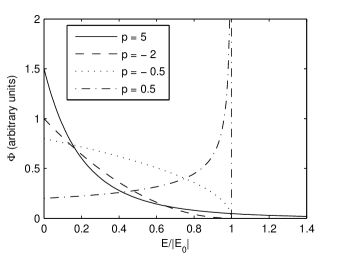
Figure 1: Qualitative behavior of the function $\Phi$ for different values of $p$.

III.2 $q$-Distributions and thermodynamics

It is easy to see that a power-law distribution can be obtained via a maximization procedure like that illustrated in Sec. II.2. In fact, if in Eq. (9) we take $F(\rho)=h^{\nu(q-1)}\rho^{q}$, where $q$ is a real number, then Eq. (12) provides

$$\Phi(E)=h^{-\nu}\left(\frac{\tilde{\alpha}+\tilde{\beta}E}{q}\right)^{1/(q-1)}\ ,$$ (27)

which coincides with Eq. (26) when putting

$$p = \frac{1}{1-q}$$ (28)

$$E_{0} = -\tilde{\alpha}/\tilde{\beta}$$ (29)

$$D = h^{\nu}|\tilde{\beta}/q|^{1/(1-q)}\ .$$ (30)

Looking at Eq. (27) one also sees that $\Phi$ will be of the form (22a) when $\tilde{\beta}/q>0$, and we have shown that in such a case the existence of a finite mean energy requires $p>1$ as a necessary condition. Viceversa, $\Phi$ will be of the form (22b) when $\tilde{\beta}/q<0$, and in that case we must then have $p<1$.

We can rewrite Eq. (9) in the form

$$\tilde{S}_{q}=h^{-\nu}\int_{\Gamma}dz\,(h^{\nu}\rho)^{q}\ ,$$ (31)

which in terms of the discrete probabilities of the quantum states becomes

$$\tilde{S}_{q}=\sum_{i}P_{i}^{q}\ .$$ (32)

According to Eq. (14) the entropy will be of the general form

$$S_{q}=kg_{q}(\tilde{S}_{q})\ ,$$ (33)

where $g_{q}$ is an appropriate monotone function which may contain $q$ as a parameter. Tsallis originally derived his power-law distribution from the function tsallis88

$$S^{T}_{q}=k\frac{1-\tilde{S}_{q}}{q-1}\ .$$ (34)

On the other hand, the expression

$$S^{R}_{q}=k\frac{\log\tilde{S}_{q}}{1-q}$$ (35)

had already been considered by Rényi in the context of information theory renyi . Other variants have also occasionally received some attention in the literature: we may here mention Tsallis normalized entropy lands

$$S^{N}_{q}=k\frac{1-\tilde{S}_{q}}{(q-1)\tilde{S}_{q}}$$ (36)

and Tsallis “escort” entropy tsescort

$$S^{E}_{q}=kq\frac{1-(\tilde{S}_{q})^{-1/q}}{1-q}\ .$$ (37)

Note that $P_{i}^{q}\sim P_{i}+(q-1)P_{i}\log P_{i}$ for $q\rightarrow 1$, whence $\tilde{S}_{q}\sim 1+(q-1)\sum_{i}P_{i}\log P_{i}$. It is then easy to see that all the four functions given in Eqs. (34)–(37) tend to the Boltzmann–Gibbs entropy (21) for $q\rightarrow 1$.

From the considerations made in Sec. II.2 it is clear that all these functions (and other possible ones) deserve equally well the name of entropy as far as the second law of thermodynamics is concerned, since for each of them one can define a state function $\beta$ such that Eq. (15) is satisfied. The criterium for the correct choice is provided in fact by the zeroth law. In the following of the present paper, after a closer analysis of the condition of thermal equilibrium between power-law distributions, we shall aim at determining the analytic form of $g_{q}$ for which $\beta$ can be expressed in the form (6), with $\Theta$ given by Eq. (4).

III.3 A generalized partition function

When a system is described by a power-law distribution of the form (26), some of the quantities previously introduced can be conveniently expressed with the aid of the auxiliary function

$$\zeta(E_{0}) = \int_{I}dE\,\omega(E)|E-E_{0}|^{1-p}$$ (38)

$$= |1-p|\int_{I}dE\,\Omega(E)|E-E_{0}|^{-p}$$

which, in the same way as an analogous one introduced in Ref. potiguar , plays the role of a generalized partition function for this class of systems. According to the considerations made in Sec. III.1, when $p>1$ the function $\zeta$ is defined for $E_{0}<0$ and the integration domain $I$ in Eq. (38) is the interval $[0,+\infty)$, whereas when $p<1$ we have $E_{0}>0$ and $I=[0,E_{0})$.

From Eq. (23) we get

$$D(E_{0})=\int_{I}dE\,\omega(E)|E-E_{0}|^{-p}=\frac{\zeta^{\prime}(E_{0})}{|1-p|}\ .$$ (39)

We can then express the function $\Theta$ defined by Eq. (4) as

$$\Theta = \frac{1}{D(E_{0})}\int_{I}dE\,\Omega(E)|E-E_{0}|^{-p}$$ (40)

$$= \frac{\zeta(E_{0})}{|1-p|D(E_{0})}=\left[\frac{d}{dE_{0}}\log\zeta(E_{0})\right]^{-1}\ .$$

We can also evaluate the mean energy $U$ using the relation

$$|U-E_{0}| = \int_{I}dE\,\omega(E)\Phi(E)|E-E_{0}|$$ (41)

$$= \frac{1}{D(E_{0})}\int_{I}dE\,\omega(E)|E-E_{0}|^{1-p}$$

$$= \frac{\zeta(E_{0})}{D(E_{0})}=|1-p|\Theta\ .$$

Since it is obviously $U>E_{0}$ (resp. $U<E_{0}$) for $p>1$ (resp. $p<1$), Eq. (41) is equivalent to

$$U=E_{0}+(p-1)\Theta\ .$$ (42)

From Eq. (31) we finally obtain

$$\tilde{S}_{q}=\frac{h^{\nu(q-1)}}{[D(E_{0})]^{q}}\int_{I}dE\,\omega(E)|E-E_{0}|^{-pq}$$

whence, using Eqs. (28), (30) and (41),

$$\tilde{S}_{q} = h^{-\nu/p}[D(E_{0})]^{1/p-1}\zeta(E_{0})$$ (43)

$$= \left|\frac{\tilde{\beta}}{q}\right|\frac{\zeta(E_{0})}{D(E_{0})}=\frac{\tilde{\beta}}{1-q}\Theta\ .$$

The expressions obtained in this subsection will be useful in the following of the paper, when we will have at our disposal an explicit expression for the function $\zeta$.

IV Power-law density-of-states functions

Let us suppose that the functions $\Omega$ of the two weakly interacting systems ${\cal S}_{1}$ and ${\cal S}_{2}$, already considered in Sec. II.1, are given respectively by $\Omega_{1}(E_{1})=B_{1}E_{1}^{s_{1}}$ and $\Omega_{2}(E_{2})=B_{2}E_{2}^{s_{2}}$, with $s_{1}>0$, $s_{2}>0$. According to Eq. (2) the function $\Omega$ for the system $\cal S$, composed of ${\cal S}_{1}$ and ${\cal S}_{2}$, is then given by

$$\Omega(E) = B_{1}B_{2}s_{1}\int_{0}^{E}dE_{1}\,E_{1}^{s_{1}-1}(E-E_{1})^{s_{2}}$$

$$= B_{1}B_{2}s_{1}E^{s_{1}+s_{2}}\int_{0}^{1}dx\,x^{s_{1}-1}(1-x)^{s_{2}}\ .$$

Since the integral in the last expression has the value $\Gamma(s_{1})\Gamma(s_{2}+1)/\Gamma(s_{1}+s_{2}+1)$ abram ; almpot , we obtain

$$\Omega(E)=BE^{s}$$ (44)

with

$$s=s_{1}+s_{2}$$ (45)

and

$$B=B_{1}B_{2}\frac{\Gamma(s_{1}+1)\Gamma(s_{2}+1)}{\Gamma(s_{1}+s_{2}+1)}\ .$$

Note that the last equation can also be put in the expressive form

$$\log[B\Gamma(s+1)]=\log[B_{1}\Gamma(s_{1}+1)]+\log[B_{2}\Gamma(s_{2}+1)]\ .$$ (46)

From Eq. (44) it also follows that $\omega(E)=BsE^{s-1}$.

Let us further assume that the system $\cal S$ is described by a power-law probability distribution of the form (26). The function $\zeta$ defined by Eq. (38) can be explicitly calculated as

$$\zeta(E_{0})=Bs\int_{I}dE\,E^{s-1}|E-E_{0}|^{1-p}=A|E_{0}|^{s-p+1}\ ,$$ (47)

where abram for $p<1$

$$A=Bs\int_{0}^{1}dx\,x^{s-1}(1-x)^{1-p}=B\frac{\Gamma(s+1)\Gamma(2-p)}{\Gamma(s-p+2)}\ ,$$ (48a)

whereas for $$p>s+1 p 1+s$$ (recall that values of between 1 and are forbidden)

$$A=Bs\int_{0}^{+\infty}dx\,\frac{x^{s-1}}{(x+1)^{p-1}}=B\frac{\Gamma(s+1)\Gamma(p-s-1)}{\Gamma(p-1)}\ .$$ (48b)

By using Eq. (39) we then obtain

$$D(E_{0})=A\frac{p-s-1}{p-1}|E_{0}|^{s-p}\ .$$ (49)

We can also calculate the marginal distribution for the subsystem ${\cal S}_{1}$ using Eq. (3a). This gives

$$\Phi_{1}(E_{1})=\frac{B_{2}s_{2}}{D}\int_{I_{1}}dE_{2}\,E_{2}^{s_{2}-1}|E_{1}+E_{2}-E_{0}|^{-p}\,$$

where $I_{1}=[0,+\infty)$ for $p>1$ and $I_{1}=[0,E_{0}-E_{1})$ for $p<1$. It is then immediate to see that

$$\Phi_{1}(E_{1})=D_{1}^{-1}|E_{1}-E_{0}|^{-p_{1}}\ ,$$ (50a)

where $$p_{1}=p-s_{2} D_{1} E_{0} B_{1} s_{1} p_{1} D E_{0} B s p$$, while the coefficient can be expressed as a function of , , , and according to the same formulae (49) and (48) which give the dependence of on , , , and . In the same way, from Eq. (3b) one finds

$$\Phi_{2}(E_{2})=D_{2}^{-1}|E_{2}-E_{0}|^{-p_{2}}$$ (50b)

with $p_{2}=p-s_{1}$. When $p<1$ it is also obvious that $\Phi_{1}(E)=\Phi_{2}(E)=0$ for $E>E_{0}$.

Equations (50) show the remarkable fact that, when the densities of states of the systems under consideration exhibit a power-law dependence on the energy, power-law probability distribution functions are compatible with the condition of thermal equilibrium which was described in Sec. II.1. We have in fact that the two weakly interacting systems ${\cal S}_{1}$ and ${\cal S}_{2}$, and the composed system $\cal S$, are all simultaneously described by stationary power-law distributions of the form (26). We note also that all these distributions have in common the same value of $E_{0}$, whilst the relation among $p_{1}$, $p_{2}$, and $p$ can be written as

$$r=r_{1}=r_{2}\ ,$$ (51)

where we have introduced the new parameter

$$r=p-s\ .$$ (52)

This means that $E_{0}$ and $r$ are intensive quantities which, like $\Theta$, assume the same value for two systems at mutual equilibrium, independently of the respective size and physical nature. From Eqs. (40) and (47) we obtain

$$\Theta=\frac{E_{0}}{1-r}\ ,$$ (53)

which implies that only two of these three quantities are actually independent. It follows that we can identify $r$ with the quantity that was introduced as a parameter of the function $f_{r}$ in Eq. (6). On the other hand, Eqs. (45) and (46) show that the quantities $s$ and $\log[B\Gamma(s+1)]$ are extensive, since their values for the complete system $\cal S$ are the sum of the corresponding values for the two subsystems ${\cal S}_{1}$ and ${\cal S}_{2}$. The same conclusions can obviously be extended to an arbitrary number of subsystems.

For the reasons that we have illustrated, systems possessing both a power-law density-of-states and a power-law probability distribution function (at least within an acceptable approximation) are likely to be the most significant ones with respect to their thermodynamic properties. In the following sections we shall refer to them shortly as “power-law systems”.

V A classification of power-law systems

Let us consider a power-law system characterized by Eqs. (44) and (26). Then from Eqs. (42) and (53) we obtain for the mean energy

$$U=\frac{s}{s-p+1}E_{0}=s\Theta\ .$$ (54)

In order to make a comparison with the Boltzmann–Gibbs distribution, let us rewrite the function $\Phi$ in the form

$$\Phi(E)=D^{-1}|E_{0}|^{-p}\exp\left[-p\log(1-E/E_{0})\right]\ .$$ (55)

For $E\ll|E_{0}|$ we have $\log(1-E/E_{0})=-E/E_{0}+O(E^{2}/E_{0}^{2})$, and the term quadratic in the energy gives a negligible contribution to the exponential function in Eq. (55) whenever

$$|p|\frac{E^{2}}{E_{0}^{2}}\ll 1\ .$$ (56)

It is now clear that, in order to evaluate the overall behavior of the statistical ensemble under consideration, only energies of the same order of magnitude as $U$ need be considered, since the probability that the system may take energy values much higher than $U$ is in general vanishingly small. If we put $E=xU=E_{0}xs/(s-p+1)$, where $x$ is a dimensionless variable, we see that the inequality $E\ll|E_{0}|$ will be satisfied for all $x$ up to order unity provided that $|p-s-1|\gg s$, whereas the condition (56) becomes equivalent to $(p-s-1)^{2}/|p|\gg s^{2}$. It is then easy to see that these two conditions will both hold only when $|p|\gg s^{2}$. Recalling Eq. (28), this is equivalent to

$$|q-1|=\frac{1}{|p|}\ll\frac{1}{s^{2}}\ .$$ (57)

In this limit we can rewrite Eq. (55) as

$$\Phi(E)\simeq D^{-1}|E_{0}|^{-p}\exp(pE/E_{0})\ ,$$ (58)

which corresponds to a canonical distribution with parameter $\beta=-p/E_{0}$. We thus find again the well-known result that a $q$-distribution tends to the Boltzmann–Gibbs distribution in the limit $q\rightarrow 1$. In addition, the above analysis gives the size of the neighborhood of 1 in which the parameter $q$ has to fall in order for the two distributions to be practically equivalent over the relevant range of energies. This size is of order $1/s^{2}$, and thus decreases as the inverse square of the dimension of the system (recall for instance that, for an ideal monoatomic gas consisting of $N$ particles, one has $s=3N/2$).

We already know from Sec. III.1 that for $0<p<1$ one has $\Phi(E)=0$ for $E>E_{0}$ and

$$\lim_{E\rightarrow E_{0}^{-}}\Phi(E)=+\infty\ .$$

Recalling Eqs. (48a) and (49) we can write for $E<E_{0}$

$$\Phi(E)=\frac{\Gamma(s-p+1)}{B\Gamma(s+1)\Gamma(1-p)}E_{0}^{p-s}(E_{0}-E)^{-p}$$

whence

$$\Phi(E)\sim\frac{1-p}{BsE_{0}^{s-1}(E_{0}-E)}\rightarrow 0\quad\text{for}\quad p\rightarrow 1^{-}\ .$$ (59)

Therefore $\Phi(E)$ vanishes in the limit $p\rightarrow 1^{-}$ for any $E\neq E_{0}$, and the probability density on the phase space becomes fully concentrated on the surface of equation $H(z)=E_{0}$. This means that the power-law distribution tends to the microcanonical ensemble in the limit $p\rightarrow 1^{-}$, which in turn corresponds to $q\rightarrow 0^{-}$. If we consider again a system ${\cal S}$ with a subsystem ${\cal S}_{1}$, and we suppose that $\cal S$ has a microcanonical distribution, so that $p\simeq 1$, then using Eq. (51) we have $p_{1}=p-s+s_{1}<1$, since $s>s_{1}$. This is in agreement with the observation, already made some years ago plastino , that a power-law distribution with finite energy cutoff may arise as the marginal of a microcanonical distribution for a finite system.

The region $s+1<p<s^{2}$ is the one in which power-law distributions display features which are most remarkably different from other known ensembles. Here the tail of the distribution at high energies becomes relevant, and represents a significant departure from the exponential decrease of the canonical ensemble. The consequences of this phenomenon become extreme in the limit $p\rightarrow(s+1)^{+}$, which corresponds to $q\rightarrow[s/(s+1)]^{+}$. Note that for macroscopic systems, having very large $s$, this limit value for $q$ still looks extremely close to 1, i.e., to the value which characterizes the Boltzmann–Gibbs distribution. Therefore $q$ does not appear to be the right parameter to distinguish among the different possible behaviors of a power-law system. To this purpose it is instead useful to introduce the parameter

$$\eta=\frac{p-1}{p-s-1}=1+\frac{s}{r-1}\ .$$ (60)

Recalling that $p$ can vary in the set $(-\infty,1)\cup(s+1,+\infty)$, we see that $\eta$ takes values in the full interval $(0,+\infty)$. The canonical ensemble, for which $q=1$, $p=\pm\infty$, corresponds to $\eta=1$; the microcanonical limit $q\rightarrow 0^{-}$, $p\rightarrow 1^{-}$ corresponds to $\eta\rightarrow 0^{+}$, and the “long power-tail” limit $p\rightarrow(s+1)^{+}$, $q\rightarrow[s/(s+1)]^{+}$ corresponds to $\eta\rightarrow+\infty$. For $0<\eta<1$ the power-law distribution is in some sense intermediate between the microcanonical and the canonical ensembles. According to the previous discussion, the behavior of the system becomes essentially canonical for $|\eta-1|\ll 1/s$. A scheme of the behavior of the parameters $p$, $q$ and $\eta$ is reported in Table 1.

Table 1: Values of the parameters $p$, $q$ and $\eta$ for the different possible types of power-law systems. Symbols $\nearrow$ and $\searrow$ indicate increase or decrease respectively.

	microcanonical				canonical		long power-tail
$p$	$1$	$\searrow$	$0$	$\searrow$	$-\infty;+\infty$	$\searrow$	$s+1$
$q$	$0$	$\searrow$	$-\infty;+\infty$	$\searrow$	$1$	$\searrow$	$s/(s+1)$
$\eta$	$0$	$\nearrow$	$1/(s+1)$	$\nearrow$	$1$	$\nearrow$	$+\infty$

Let us write down the relation between the parameters $\eta$ and $\eta_{1}$ of two systems $\cal S$ and ${\cal S}_{1}$ at equilibrium with each other. Since $r-1=s/(\eta-1)$, from Eq. (51) we obtain

$$\eta_{1}=1+\frac{s_{1}}{r_{1}-1}=1+s_{1}\frac{\eta-1}{s}\ .$$ (61)

If we now consider a large power-law system $\cal S$ composed of many weakly interacting microscopical particles, it is interesting to take as ${\cal S}_{1}$ the subsystem constituted by a single particle, for which the parameter $s_{1}$ is typically of order unity (for an ideal monoatomic gas one has for instance $s=3N/2$, $s_{1}=3/2$). According to the previous analysis, the one-particle distribution will be appreciably different from Boltzmann–Gibbs when $|\eta_{1}-1|\geq 1/s_{1}=O(1)$, which on account of Eq. (61) is equivalent to $|\eta-1|s_{1}/s\geq O(1)$. For $s\gg s_{1}$ this can clearly occur only when $\eta\geq s$, which corresponds to a system $\cal S$ far in the long power-tail regime.

VI Thermodynamic functions of power-law systems

VI.1 Temperature and entropy

Let us now consider the crucial problem of determining the thermodynamic temperature and entropy of a power-law system. According to Eqs. (6) and (16) we must have

$$\beta=f_{r}(\Theta)=\tilde{\beta}g^{\prime}_{q}(\tilde{S}_{q})\ .$$ (62)

Taking into account Eq. (43), the above equation can be rewritten in the form

$$\Theta f_{r}(\Theta)=(1-q)\tilde{S}_{q}g^{\prime}_{q}(\tilde{S}_{q})\ .$$ (63)

When we introduced the function $g_{q}(\tilde{S}_{q})$ in Eq. (33), we made the assumption that it may contain the only parameter $q$ (see the last part of Appendix A for some related considerations). We then observe that the two variables $r$ and $\Theta$, that appear on the left hand side of Eq. (63), are independent of the two variables $q$ and $\tilde{S}_{q}$ that appear on the right hand side. It can in fact be easily checked (see Appendix A) that all these four quantities can be expressed as independent functions of the four free parameters $p$, $E_{0}$, $s$, and $B$ that characterize the system according to Eqs. (26) and (44). It is then obvious that the two members of Eq. (63) can be identically equal to each other only if they are both equal to a common constant value $c$. If we first consider the second member, we can thus write

$$g^{\prime}_{q}(\tilde{S}_{q})=\frac{c}{(1-q)\tilde{S}_{q}}\ .$$ (64)

Integrating this equation and recalling Eq. (33), we obtain that the entropy $S_{q}$ of the power-law system is given by

$$S_{q}=kg_{q}(\tilde{S}_{q})=ck\frac{\log\tilde{S}_{q}}{1-q}+I(q)\ ,$$ (65)

where $I(q)$ is an a priori arbitrary function of $q$. The requirement that the Boltzmann–Gibbs expression (21) has to be recovered in the limit $q\rightarrow 1$ imposes the conditions $c=1$ and $I(1)=0$. If we further require that, in accordance with the third law of thermodynamics, the entropy vanishes at zero temperature for all systems with a nondegenerate ground state, we must set $I(q)=0$ for any $q$. In this way we finally obtain

$$S_{q}=k\frac{\log\tilde{S}_{q}}{1-q}\ ,$$ (66)

which coincides with the expression of Rényi entropy $S_{q}^{R}$ given by Eq. (35).

Setting also the left-hand side of Eq. (63) equal to 1 provides the expression for the inverse absolute temperature:

$$\frac{1}{kT}\equiv\beta=f_{r}(\Theta)=\frac{1}{\Theta}\ .$$ (67)

We therefore find that the relation $kT=\Theta$, which had already been proved for the Boltzmann–Gibbs statistics, is valid for all power-law systems. From Eqs. (53) and (54) we also find for the mean energy $U$ of the system the value

$$U=\frac{s}{\beta}=skT\ .$$ (68)

As in standard thermodynamics, the energy is thus directly proportional to the absolute temperature $T$, and the specific heat at constant volume is given by

$$C_{V}\equiv\frac{\partial U}{\partial T}=sk\ .$$ (69)

As a verification of the results obtained in this section, we examine in Appendix B the consequences of adopting, instead of Eq. (35), the three different entropies mentioned at the end of Sec. III.2.

VI.2 Properties of Rényi entropy

On account of the results of the previous subsection, from now on we shall directly write $S_{q}^{R}$ in place of $S_{q}$. From Eqs. (43), (30), (49) and (53) we obtain

$$k^{-1}S_{q}^{R} = -\nu\log h+\log A+(p-1)\log\frac{p-1}{p-s-1}$$ (70)

$$+\ s\log(|p-s-1|kT)\ .$$

Having in mind that the number of degrees of freedom $\nu$ and the value of the external quantities such as the volume are directly related to the parameters $s$ and $B$ of the density of states (44), and recalling Eq. (28), we want here to analyze the behavior of the entropy considered as a function of the independent variables $q$, $s$, $B$, and $T$.

Let us first of all compare Eq. (70) with the corresponding expression for the Boltzmann–Gibbs entropy. By substituting for $\rho=\Phi(E)$ the expression (19) into Eq. (20), and observing that, on account of Eq. (44),

$$Z = \int_{\Gamma}dz\,e^{-\beta H}=\int_{0}^{+\infty}dE\,sBE^{s-1}e^{-\beta E}$$

$$= \beta^{-s}B\Gamma(s+1)\ ,$$

one obtains

$$k^{-1}S_{BG}(s,B,T)=-\nu\log h+\log[B\Gamma(s+1)]+s\log kT+s\ .$$ (71)

We can write in general

$$S^{R}_{q}(s,B,T)=S_{BG}(s,B,T)+\Delta S_{q}(s)\ ,$$ (72)

where, using for $A$ the expressions (48), we have

$$k^{-1}\Delta S_{q}(s) = \log\frac{\Gamma(1-p)}{\Gamma(s+1-p)}+p\log(1-p)$$ (73a)

$$+\ (s-p)\log(s+1-p)-s$$

for $$p<1$$, and

$$k^{-1}\Delta S_{q}(s) = \log\frac{\Gamma(p-s)}{\Gamma(p)}+p\log(p-1)$$ (73b)

$$-\ (p-s)\log(p-s-1)-s$$

for $p>s+1$. By calculating the limit of the expression (73a) for $p\rightarrow-\infty$ and the limit of (73b) for $p\rightarrow+\infty$ one can easily check that $\lim_{q\rightarrow 1}\Delta S_{q}(s)=0$. We can therefore conclude that, as expected,

$$\lim_{q\rightarrow 1}S_{q}^{R}(s,B,T)=S_{BG}(s,B,T)\ .$$

Another interesting case to consider is the limit $q\rightarrow 0^{-}$, or $p\rightarrow 1^{-}$, which according to our discussion of Sec. V corresponds to a microcanonical distribution. Taking into account Eq. (68) we obtain from Eqs. (71) and (73a)

$$\lim_{q\rightarrow 0}S_{q}^{R}(s,B,T) = k(-\nu\log h+\log B+s\log U)$$ (74)

$$= k\log\frac{\Omega(U)}{h^{\nu}}\ ,$$

which is indeed a well-known expression for the entropy in the microcanonical ensemble gibbs ; munster .

Since the expression (71) is manifestly extensive, in order to investigate the thermodynamic limit it is only necessary to study the behavior of $\Delta S_{q}$ for $s\rightarrow+\infty$. If we treat $q$ (and therefore also $p$) as a constant, recalling that $p$ can never lie in the interval $[1,s+1]$ we see that such a limit can only be taken when $p<1$. Therefore, applying Stirling’s formula to the expression (73a) we obtain

$$\Delta S_{q}(s)\sim-\frac{3}{2}k\log s\quad\text{for}\quad s\rightarrow+\infty\ .$$ (75)

From a physical point of view it might seem more appropriate to consider a thermodynamic limit in which the intensive quantity $r$ is kept constant instead of $q$. We have in this case $p=s+r\rightarrow+\infty$, which implies $p>s+1$. Then from Eq. (73b) we obtain

$$\Delta S_{q}(s)\sim-\frac{1}{2}k\log s\quad\text{for}\quad s\rightarrow+\infty$$ (76)

with $r=$ constant, $q=1-1/(s+r)\rightarrow 1^{-}$.

Let us finally consider the thermodynamic limit in which we keep constant the parameter $\eta$ introduced in Sec. V. We have in this case to substitute $p=\eta s/(\eta-1)+1$ into Eq. (73a) when $0<\eta<1$, or into Eq. (73b) when $\eta>1$, and then to take the limit for $s\rightarrow+\infty$. We obtain in this way

$$\lim_{s\rightarrow+\infty}\Delta S_{q}(s)=\begin{cases}\frac{3}{2}k\log\eta\quad&\text{for}\quad 0<\eta<1\\ -\frac{1}{2}k\log\eta\quad&\text{for}\quad\eta\geq 1\end{cases}$$ (77)

with $\eta=$ constant, $q=s/(s+1-\eta^{-1})\rightarrow 1$.

We see that in the limits considered $\Delta S_{q}$ either increases logarithmically with the size of the system, as in Eqs. (75)–(76), or tends to a constant value as in Eq. (77). It follows that in all cases the extensive part $S_{BG}$ prevails in Eq. (72), and the entropy $S_{q}^{R}(s,B,T)$ essentially reduces to $S_{BG}(s,B,T)$ as $s\rightarrow+\infty$. We note also that $q$ does not appear in the expression (68) of the mean energy. These results can be seen as a generalization of the well-known theorem about the equivalence of the different ensembles in the thermodynamic limit. We have shown in fact that this equivalence does not only hold between the canonical and the microcanonical ensembles, but also among the power-law distributions corresponding to all possible values of $\eta$. This fact is all the more remarkable if one recalls that, as we have illustrated in detail in Sec. V, the microscopical distribution function can instead be significantly different from Boltzmann–Gibbs also for very large systems.

We would like finally to mention that the additivity of Rényi entropy for mutually independent systems was already well known. Our analysis has shown on the other hand that it is also additive for large power-law systems which, instead of being independent, are at mutual thermal equilibrium in the sense that we have specified in Sec. II.1. One can observe nevertheless that the Rényi entropy (72) includes, at variance with the Boltzmann–Gibbs one, a nonextensive contribution $\Delta S_{q}$ which may be nonnegligible for systems of small size.

VI.3 The ideal gas

Let us consider as a significant example the case of an ideal monoatomic gas composed of $N$ particles of mass $m$ in a volume $V$. We have

$$\nu = 3N$$

$$s = \frac{3N}{2}$$

$$B = \frac{(2\pi m)^{3N/2}V^{N}}{\Gamma(3N/2+1)N!}\ ,$$

where the factor $N!$ in the denominator of the last expression accounts for the indistinguishability of the atoms. From Eqs. (68) and (71) we then obtain for large $N$

$$U = \frac{3}{2}NkT$$ (78)

$$S^{R}_{q} = Nk\left[\frac{3}{2}\log\frac{2\pi mkT}{h^{2}}+\log\frac{V}{N}+\frac{5}{2}\right]$$ (79)

$$+\ O(\log N)\ .$$

We find in this way two formulae which are already familiar from standard statistical thermodynamics. It is then easy to see that ideal gases governed by power-law distributions obey the same state equation of Boltzmann–Gibbs ideal gases. Consider in fact an infinitesimal isothermal transformation, for which $dT=0$. Then from Eq. (78) we get $dU=0$, and the infinitesimal work $\delta W=PdV$ performed by the system, where $P$ is the pressure of the gas, can be obtained according to the first and second laws of thermodynamics as

$$PdV=\delta Q=TdS_{q}^{R}=NkT\frac{dV}{V}\ ,$$ (80)

where the last equality follows from Eq. (79). Comparing the first and last members of the above equation we finally get

$$PV=NkT\ .$$ (81)

In particular, one can conclude that also for power-law systems the ideal gas temperature defined according to Eq. (81) is the same as the thermodynamic temperature based on the second law.

VII Conclusion

We have developed a new generalized thermodynamics for systems governed by Tsallis distributions, in a way which also allows for a rigorous statistical interpretation of the zeroth law. Our approach thus provides a new point of view on an issue which has been the object of sharp debate in recent literature nauen . The main outcome of our analysis is that the thermodynamic entropy associated with these distributions is expressible as a function of the probabilities according to the formula first introduced by Rényi.

Our results have been obtained under a minimum set of simple and apparently plausible hypotheses. Probably the main new ingredient, with respect to former investigations, is the observation that Tsallis statistics is capable of describing stationary states, in which power-law systems combine together in such a way to give rise to a larger composed power-law system. The consideration of such a circumstance allows one to extend to a deeper level the analogy with the standard thermodynamics of weakly interacting systems gibbs ; khin , which has already proved to be an illuminating guideline for the analysis of Tsallis thermostatistics plastino ; almeida1 ; adib ; almpot ; potiguar ; almeida .

Of course power-law distributions can in principle apply also to systems for which the hypotheses of weak coupling or of power-law density of states are in general not satisfied. An important case of this type is likely to be represented by systems of particles with long-range interactions, which are indeed considered among the most interesting candidates for the applicability of nonextensive thermodynamics. In such cases the conclusions of our analysis may not necessarily hold, and it is possible that other theoretical investigations are to be carried out on the basis of a completely different approach. In particular, other descriptions might become appropriate, in which no reference at all is made to the usual formalism of equilibrium thermodynamics. For instance, a justification for Tsallis entropy has recently been proposed on the basis of purely dynamical assumptions about the behavior of a system far from equilibrium carati1 . It has also been pointed out that deviations from the exact Tsallis distribution law can be present in real situations beck . It is reasonable to expect that such deviations may be related to the specific form of the density-of-states function, so that a generalization of Tsallis statistics might be required in order to treat the cases in which the density of states significantly departs from a power law.

Appendix A On the independent parameters of a power-law system

The deduction of Eq. (64) from Eq. (63) is based on the mutual independence of the four variables $r$, $\Theta$, $q$ and $\tilde{S}_{q}$. In order to elucidate this point, let us start from the four main free parameters which can be put at the basis of the description of a power-law system. These are $s$, $B$, $p$ and $E_{0}$. The first two of them appear in the expression (44) which gives the primitive function of the density of states, and are therefore directly related to the form of the hamiltonian function. Their physical meaning is illustrated by the example of the ideal gas which is treated in Sec. VI.3. In particular, $2s$ expresses the number of degrees of freedom contributing to the hamiltonian, and is therefore related to the size (number of particles) of the system, while $B$ contains the dependence on the external parameters which, like the volume $V$, are varied when the system exchanges mechanical work with the surrounding environment. On the other hand, $p$ and $E_{0}$ are the two free parameters in the power-law probability distribution (26), $D$ being a normalization constant. According to Eqs. (28) and (54), $p$ is simply a function of $q$, while $E_{0}$ fixes the mean energy, and thus the temperature of the distribution. For the case of the ideal gas, for instance, the mutual independence of $s$, $B$, $E_{0}$ and $p$ amounts to the mutual independence of $N$, $V$, $T$ and $q$.

Assuming for simplicity the relation $\nu=2s$ as for the ideal gas (the particular relation between these two parameters is inessential with respect to the present considerations), we can express $q$, $r$, $\Theta$ and $\tilde{S}_{q}$ as functions of the independent quantities $s$, $B$, $E_{0}$ and $p$, according to the relations

$$q = 1-\frac{1}{p}$$ (82)

$$r = p-s$$ (83)

$$\Theta = \frac{E_{0}}{1+s-p}$$ (84)

$$\tilde{S}_{q} = \frac{1-p}{s+1-p}\left(BG(s,p)\Gamma(s+1)\frac{|E_{0}|^{s}}{h^{2s}}\right)^{1/p}$$ (85)

Equations (82)–(84) are identical respectively to Eqs. (28), (52) and (53). Equation (85), in which we have introduced the function

$$G(s,p)\equiv\begin{cases}\Gamma(1-p)/\Gamma(s-p+1)\quad&\text{for}\quad p<1\\ \Gamma(p-s)/\Gamma(p)\quad&\text{for}\quad p>s+1\ ,\end{cases}$$

is derived from Eqs. (43) and (47)–(49).

It easy to see that the four functions defined by Eqs. (82)–(85) are mutually independent. They can in fact be explicitly inverted, so as to express $s$, $p$, $E_{0}$ and $B$ as functions of $q$, $r$, $\Theta$ and $\tilde{S}_{q}$. We obtain

$$s = \frac{1}{1-q}-r$$ (86)

$$p = \frac{1}{1-q}$$ (87)

$$E_{0} = (1-r)\Theta$$ (88)

$$B = \frac{K(q,r)}{\Gamma(1/(1-q)-r+1)}$$ (89)

$$\times\left(\frac{(q-1)(1-r)}{q}\tilde{S}_{q}\right)^{1/(1-q)}$$

$$\times\left(\frac{h^{2}}{\Theta|1-r|}\right)^{1/(1-q)-r}\ ,$$

where

$$K(q,r)\equiv\begin{cases}\displaystyle{\frac{\Gamma(1-r)}{\Gamma(q/(q-1))}}\quad&\text{for}\quad q<0,\ q>1\\[8.0pt] \displaystyle{\frac{\Gamma(1/(1-q))}{\Gamma(r)}}\quad&\text{for}\quad\displaystyle{\frac{s}{s+1}}<q<1\ .\end{cases}$$

The argument we have used after Eq. (63), in order to justify the introduction of the constant $c$, is also based on the assumption that the function $g_{q}(\tilde{S}_{q})$ does not contain any parameter other than $q$. Note that all the functions appearing on the right-hand sides of Eqs. (34)–(37) do agree with this general assumption, which is dictated by obvious reasons of simplicity and economy. We expect in fact that such a fundamental physical quantity as the entropy should have the simplest analytical expression which is compatible with the laws of thermodynamics, without the inclusion of unnecessary parameters. The argument about the constancy of $c$ is also at the basis of the remarkable equality, which we have found in Sec. VI.1, between the “empirical temperature” $\Theta$ and the thermodynamic temperature $kT$. It is however interesting to examine the consequences of restraining from the above assumption, and considering in Eq. (33) a function $g_{q,r}(\tilde{S}_{q})$ which may also depends on the parameter $r$. This would imply the replacement of the constant $c$ on the right-hand side of Eq. (65) with a function $c(r)$, which would then remain as a multiplicative coefficient also in the final expressions of the entropy and of the inverse temperature:

$$S_{q}=kc(r)\frac{\log\tilde{S}_{q}}{1-q}\ ,\qquad\qquad T=\frac{\Theta}{kc(r)}\ .$$

Taking into account Eqs. (83) and (87), one should then be forced to require that $\lim_{r\to\pm\infty}c(r)=1$, in order for the Boltzmann–Gibbs entropy and temperature to be recovered in the limit $q\to 1$. Furthermore, we have shown in Sec. V that a power-law distribution tends to the microcanonical ensemble for $q\to 0$. If one then requires that the correct microcanonical entropy (74) and the empirical temperature $kT=\Theta=U/s$ munster be obtained for any $s>0$ in the limit $q\to 0$, it would also be necessary to impose $c(r)=1$ for all $r$ such that $-\infty<r<1$. These can be considered as additional arguments in favor of the natural choice of taking $c=1$ for all $r$.

Appendix B Comparison among alternative entropies

In Sec. VI.1 we have proved that the condition of compatibility with the zeroth law of thermodynamics univocally determines the expression of the entropy for a power-law system. As a verification of this result, it is interesting to check directly how this condition of compatibility is violated by the three particular functions which have been mentioned at the end of Sec. III.2 as well-known possible alternatives to Rényi entropy.

It follows from the first and second laws of thermodynamics that the inverse of the thermodynamic temperature $\beta$ must be related to the entropy $S$ by the equation

$$k\beta=\frac{\partial S}{\partial U}\ ,$$ (90)

where the partial derivative of the entropy is evaluated at constant external parameters (i.e., those parameters, such as the volume of the system, whose variation is related to the production of mechanical work). When the entropy has the form (33) we have then

$$\beta=g^{\prime}_{q}(\tilde{S}_{q})\frac{\partial\tilde{S}_{q}}{\partial U}\ .$$ (91)

From Eqs. (43), (47), (49) and (54) we obtain

$$\tilde{S}_{q}=\left[h^{-\nu}A\left(\frac{p-1}{p-s-1}\right)^{p-1}\left(\frac{|p-s-1|}{s}U\right)^{s}\right]^{1/p}\ .$$

According to Eq. (48), the quantity $A$ depends on the external parameters (through $B$) but not on the internal energy $U$. We therefore obtain

$$\frac{\partial\tilde{S}_{q}}{\partial U}=\frac{s\tilde{S}_{q}}{pU}=\frac{\tilde{S}_{q}}{p\Theta}\ .$$

Substituting for $g^{\prime}_{q}$ in Eq. (91) the derivatives of the expressions which appear on the right-hand sides of Eqs. (34)–(37), we then find for the function $\beta$ in the four respective cases

$$\beta^{T} = \frac{\tilde{S}_{q}}{\Theta}$$

$$\beta^{R} = \frac{1}{\Theta}$$

$$\beta^{N} = \frac{1}{\tilde{S}_{q}\Theta}$$

$$\beta^{E} = \frac{1}{\tilde{S}_{q}^{1/q}\Theta}\ .$$

We thus see that only $\beta^{R}$, derived from Rényi entropy, is equal to the inverse of the parameter $\Theta$ which was introduced in Sec. II.1 on the basis of the zeroth law of thermodynamics. On the contrary, $\beta^{T}$, $\beta^{N}$ and $\beta^{S}$, which are respectively associated with the entropies (34), (36) and (37), depend also on $\tilde{S}_{q}$, which in general takes different values for systems at thermal equilibrium with each other. It is therefore confirmed, by the analysis of these examples, that only Rényi entropy leads to an expression for the thermodynamical temperature which is compatible with the zeroth law. This result obviously does not exclude that Tsallis or other entropies can nevertheless be conveniently employed whenever some of the starting hypotheses of the present work (such as weak coupling or power-law density of states) are manifestly violated by the system under investigation. In such circumstances a proper modification of the standard laws of thermodynamics will also be necessary, as it has already been recognized in the literature.

References

- (1) S. Abe and Y. Okamoto (eds.), “Nonextensive Statistical Mechanics and its Applications,” Lecture Notes in Physics Vol. 560, Springer-Verlag, Berlin, 2001.
- (2) C. Tsallis and E. Brigatti, Continuum Mech. Thermodyn. 16, 223 (2004), and references therein.
- (3) M. Gell-Mann and C. Tsallis (eds.), “Nonextensive Entropy — Interdisciplinary Applications,” Oxford University Press, New York, 2004.
- (4) C. Beck, G. Benedek, A. Rapisarda and C. Tsallis (eds.), “Complexity, Metastability and Nonextensivity,” World Scientific, Singapore, 2005.
- (5) G. Kaniadakis, A. Carbone and M. Lissia (eds.), “Fundamental Problems in Modern Statistical Mechanics,” Physica A, Vol. 365, Issue 1, 2006; “Modern Problems in Complexity,” European Physical Journal B, Vol. 50, No. 1-2, 2006.
- (6) See http://tsallis.cat.cbpf.br/biblio.htm for a regularly updated bibliography.
- (7) C. Tsallis, J. Stat. Phys. 52, 479 (1988).
- (8) S. Abe, S. Martínez, F. Pennini and A. Plastino, Phys. Lett. A 281, 126 (2001).
- (9) C. Beck and E. G. D. Cohen, Physica A 322, 267 (2003).
- (10) C. Vignat and A. Plastino, Comptes Rendus Phys. 7, 442 (2006).
- (11) A. R. Plastino and A. Plastino, Phys. Lett. A 193, 140 (1994).
- (12) M. P. Almeida, Physica A 300, 424 (2001).
- (13) A. A. Adib, A. A. Moreira, J. S. Andrade Jr. and M. P. Almeida, Physica A 322, 276 (2003).
- (14) M. P. Almeida, F. Q. Potiguar and U. M. S. Costa, “Microscopic analog of temperature with nonextensive thermostatistics,” cond-mat/0206243 (2002).
- (15) F. Q. Potiguar and U. M. S. Costa, “Thermodynamics arising from Tsallis’ thermostatistics,” cond-mat/0208357 (2002).
- (16) M. P. Almeida, Physica A 325, 426 (2003).
- (17) J. W. Gibbs, “Elementary Principles in Statistical Mechanics,” Yale University Press, 1902; reprinted by Dover, New York, 1960.
- (18) A. I. Khinchin, “Mathematical Foundations of Statistical Mechanics,” Dover, New York, 1949.
- (19) A. Rényi, in “Proceedings of the Fourth Berkeley Symposium on Mathematical Statistics and Probability,” Vol. I, University of California Press, Berkeley, 1960.
- (20) A. Rényi, “Probability Theory,” North-Holland, Amsterdam, 1970.
- (21) A. Münster, “Statistical Thermodynamics,” Springer Verlag, Berlin, 1969.
- (22) E. M. F. Curado and C. Tsallis, J. Phys. A 24, L69 (1991).
- (23) P. T. Landsberg and V. Vedral, Phys. Lett. A 247, 211 (1998); A. K. Rajagopal and S. Abe, Phys. Rev. Lett. 83, 1711 (1999).
- (24) C. Tsallis, R. S. Mendes and A. R. Plastino, Physica A 261, 534 (1998).
- (25) M. Abramowitz and I. A. Stegun, “Handbook of Mathematical Functions,” page 258, Dover, New York, 1968.
- (26) M. Nauenberg, Phys. Rev. E 67, 036114 (2003); C. Tsallis, Phys. Rev. E 69, 038101 (2004); M. Nauenberg, Phys. Rev. E 69, 038102 (2004).
- (27) A. Carati, Physica A 348, 110 (2005); 369, 417 (2006).