Abstract

We consider the level statistics of two-dimensional harmonic oscillators with incommensurable frequencies, which are known to have picket-fence type spectra. We propose a parametric representation for the level-spacing distribution and level-number variance, and study the variation of the parameters with the frequency ratio and the size of the spectra. By introducing an anharmonic perturbation, we observe a gradual transition to the Poisson statistics. We describe the level spectra in transition from harmonic to Poissonian statistics as a superposition of two independent sequences, one for each of the two extreme statistics. We show that this transition provides a suitable description for the evolution of the spectrum of a disordered chain with increasing long range correlations between the lattice sites.

PACS numbers: 03.65-w, 05.45.Mt, 05.30.

1 INTRODUCTION

Bohigas, Giannoni and Schmidt [1] have conjectured that the spectral fluctuations of a quantum system whose classical analog is chaotic follows the predictions of the random matrix theory [2]. This conjecture has been checked numerically on a wide variety of systems (for recent reviews, see e.g. [3, 4]). The spectra of classically integrable quantum systems are admitted as a sequence of uncorrelated levels that follows the Poisson statistics. Berry and Tabor [5] have given elaborate semiclassical arguments in favor of this admission. The Poisson distribution for regular spectra has been proven in some cases (see results by Sinai [6] and Marklof [7], for instance).

Not all of the integrable systems have a Poissonian level-spacing distribution. The two-dimensional harmonic oscillator is a classical example. Berry and Tabor [5] show that the spacing distribution does not exist if the oscillator frequencies are commensurable. It is peaked at a non-zero value if the frequencies are incommensurable. The spectrum in this case has nearly a picket-fence shape. The reason for this anomalous behavior is the following. Berry and Tabor [5] obtain the Poissonian level-spacing distribution by assuming curved energy contours in the action space and applying the stationary phase method. For the harmonic oscillator the energy contours are flat and the method breaks down. Subsequent studies of the energy spectra of harmonic oscillators are essentially a continuation of [5]. Pandey and collaborators [8, 9] use number theory to show that harmonic oscillators have a strong level repulsion and no fixed spacing distribution. A stable limit for the level-spacing distribution is obtained using special averaging techniques by Greenman [10]. More recently, Chakrabati and Hu [11] demonstrate by numerical calculation that the spacing distribution settles into a stable distribution as the number of involved levels exceeds 5000. The existence and the stability of the form of the spacing distribution of the irrational two-dimensional oscillator call for further investigations.

Because of its mathematical simplicity, the harmonic oscillator provides solvable models in many branches of physics. It often gives illustrations of abstract ideas. Nevertheless, the spectral fluctuations of the oscillator have not been studied carefully enough in the more than quarter-of-a-century that elapsed since the publication of the work by Perry and Tabor. Recently, picket-fence-like spectra have been observed in several elaborate numerical experiments such as quantum graphs [12]. The development of spectra of correlated disordered chains under the influence of long range correlation, reported in [13], may be regarded as an evolution from the Poissonian behavior towards that of a picket fence. This provides an additional reason for revisiting the irrational two-dimensional oscillator.

The aim of the present paper is to further explore the spectrum of the two-dimensional oscillator, particularly when it is subject to a small departure from harmonicity. Section 2 is devoted to the numerical investigation of the spectral fluctuations of the oscillators in terms of their level-spacing distributions and level-number variances. Section 3 shows that the violation of the harmonicity of the oscillators results in a transition to the Poissonian statistics. Section 4 describes the evolution of the spectra of a one-dimensional lattice of a large number of sites interacting according to a tight-binding hamiltonian under the influence of long range correlations, observed in [13], as a transition from the Poissonian to the harmonic behavior. The conclusions of this work are summarized in Section 5.

2 The two-dimensional oscillator

In this section, we add a small contribution to the study of energy spectra of two-dimensional harmonic oscillators, initiated by Berry and Tabor [5]. The energy eigenvalues for such a system are given by

$$E_{i}^{harmonic}=\hbar\omega(n+\alpha m),\$$ (1)

where $\omega$ is the larger frequency and $\alpha$ is the frequency ratio while $i$ stands for the quantum-number pair $n$ and $m$.

We can represent each state by a point in the first quadrant of the plane whose axes represent the quantum numbers $n$ and $m$. For $\hbar\omega=1$, the number of states below some energy $E$ is equal to the number of points in the first quadrant below the straight line cutting the $n$-axis at $E$ and the $m$-axis at $E/\alpha$. Thus, the number of states below some energy $E$ is proportional to $E^{2}$, the density of states increases linearly with $E$, and the mean level spacing is proportional to $1/E$.

Although the two-dimensional harmonic oscillator is an integrable system, its nearest neighbor spacing distribution does not follow the Poisson distribution characteristic of generic regular systems. Berry and Tabor [5] showed that the spacing distribution $P(s)$ does not exist if $\alpha$ is a rational number. For irrational values of $\alpha$, they calculated 10 000 eigenvalues and constructed the histograms of $P(s)$ for oscillators with $\alpha=1/\sqrt{2},1/\sqrt{5},e^{-1}$ and $\pi^{-1}$. In the first three cases, the obtained $P(s)$ is tightly peaked at $s=1$ and shows weak dependence on the frequency ratio. According to these authors, the spacing distributions show similar behavior for $\alpha=1/\sqrt{3},1/\sqrt{7}$ and $(\sqrt{5}-1)/2$. In the case of $\alpha=\pi^{-1}$, however, the distribution is bimodal with peaks at $s$ = 0.5 and 4.3, which has been attributed to the close equality of $\pi$ to many rational numbers.

In further studies of the irrational two-dimensional oscillator by Pandey and collaborators [8, 9], it was shown, using number theory arguments, that in any integer segment $[M,M+1]$ of the energy spectrum there are at most three spikes in the spacing distributions of these integer segments. They also argued that the spacing distributions do not reach stability at all, while numerical studies by Chakrabati and Hu [11] suggest that stability is reached when the number of states is about 5000.

In Fig. 1, we show the spacing distributions for the irrational two-dimensional oscillator with $\alpha=1/\sqrt{5}$. Left histograms show the spacing distributions for successive 1000 levels, while the right ones show the spacing distributions for the lowest 1000, 2000, …, and 10000 levels. The left histograms of Fig. 1 show the spike structure [8, 9] even though 1000 states cover more than one unit segment of the energy spectrum. The $N=5000$ and $N=10000$ histograms of the right part of Fig. 1 show that the spacing distribution does not reach stability when the number of states reach 5000 as claimed by Chakrabati and Hu [11].

Berry and Tabor [5] stated that they were not able to prove that for any irrational oscillator that the level spacing distributions settle into a stable form, but they also stated that their numerical results suggest that they do.

Our numerical results displayed in Fig. 1 show that the positions of the spikes in the spacing distributions change from one interval to another. Adding the contributions from different intervals, we notice that the spike structure disappears and the fluctuations in the spacing distributions may not qualitatively change the shape of the distribution for sufficiently large $N$. We also notice that the spacing distribution tends to be peaked around $s=1$.

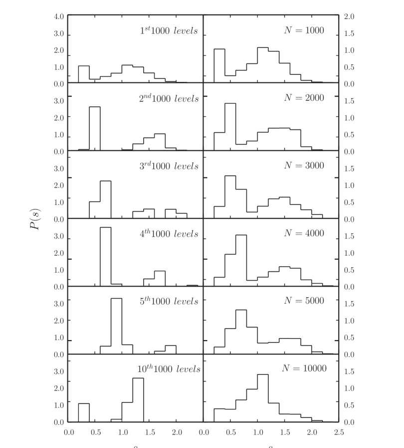
Figure 1: Left histograms : level spacing distributions for 1000 successive levels. Right histograms : level spacing distributions for the lowest 1000, 2000, …, 10000 levels. All histograms are for the irrational oscillator of Eq. (1) with $\alpha=1/\sqrt{5}$. One should note that the vertical left and right scales are different.

We would like to test the dependence of spectral fluctuations on the number $N$ of levels constituting the spectrum and the frequency ratio $\alpha$. We show the results for $P(s)$ for the first $N$ levels of the oscillators with $\alpha=1/\sqrt{2}$ in Fig. 2, where $N$ is increased from 1000 to 10 000 by steps of 1000. The spectra are unfolded using a cubic polynomial. They are fitted to a modified Gaussian distribution

$$P(s,w)=\frac{1}{\sqrt{\pi}w{\rm{Erf}}(1/w)}\left[e^{-(s-s_{c})^{2}/w^{2}}-e^{-(s+s_{c})^{2}/w^{2}}\right],\$$ (2)

where Erf($x$) is the error function, $w>$ 0. This distribution vanishes at the origin and has a mean value of $s_{c}$. The pre-factor takes care of the normalization condition. In our numerical analysis, we fixed the mean spacing at $s_{c}$ = 1. The widths, however, are allowed to vary.

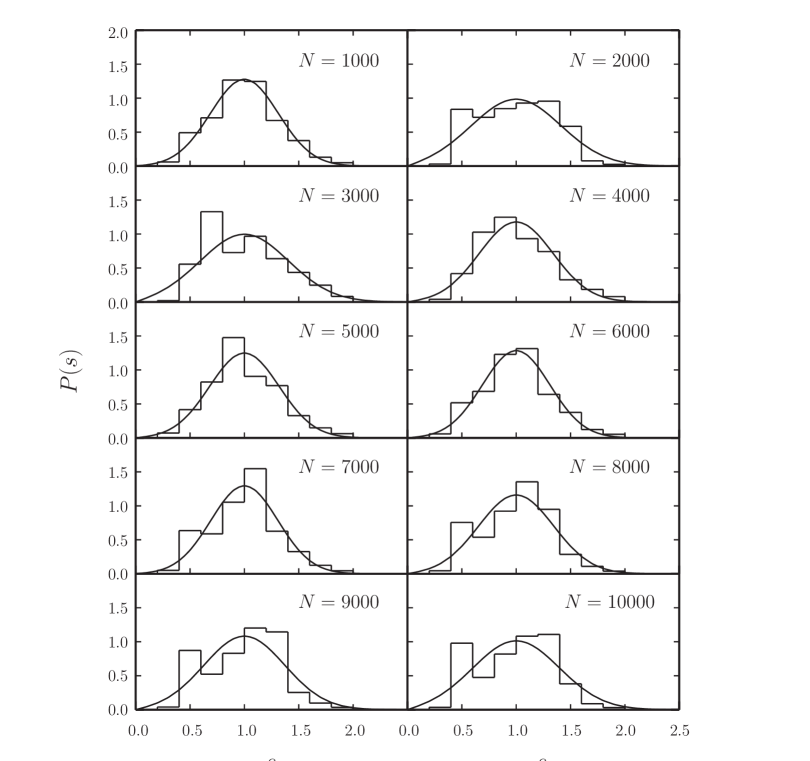
Figure 2: Level spacing distributions for the first 1000, 2000, …, 10000 levels of the irrational oscillator of Eq. (1) with $\alpha=1/\sqrt{2}$, fitted to the modified Gaussian distribution of Eq. (2).

We have also done the calculation for other values of $\alpha=1/\sqrt{5},1/\sqrt{7}$. The best-fit values of the width parameter $w$ are given in Fig. 3. The figure suggests that the values of $w$ show regular oscillation with increasing $N$ about a mean value that depends on the frequency ratio. The mean values and the standard deviations are $w$ = 0.50 $\pm$ 0.06, 0.71 $\pm$ 0.18, 0.52 $\pm$ 0.12, for $\alpha=1/\sqrt{2},1/\sqrt{5},1/\sqrt{7}$, respectively. Nevertheless, we can say that the best-fit values of $w$ agree within the error bars which are less than 25$\%$.

We have also evaluated the number variance $\Sigma_{2}$ for the same spectra. The level number variance is given by

$$\Sigma_{2}(r)=<n^{2}(r,x)>-\left<n(r,x)\right>^{2},\$$ (3)

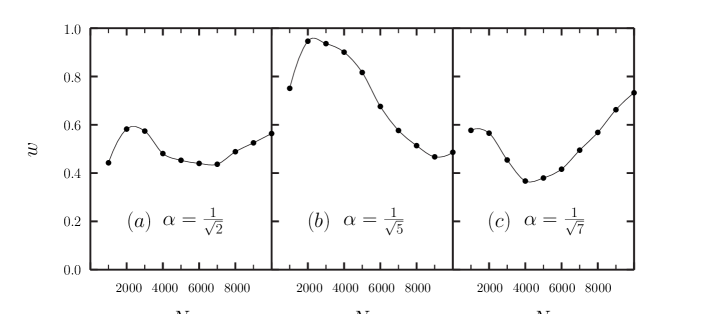
Figure 3: Dependence of the parameter $w$ of the modified Gaussian distribution of Eq. (2) on the size of the spectra for $\alpha=1/\sqrt{2}$, $1/\sqrt{5}$, and $1/\sqrt{7}$.

where $n(r,x)$ counts the number of levels in the interval $[x,x+r]$ on the unfolded scale. The angular brackets in Eq. (3) denotes the averaging over the initial energies $x$.

In Ref. [14] the spectral rigidity for a Gaussian orthogonal ensemble of random matrices was successfully fitted by a three-parameter formula, which was designed in accordance with the asymptotic form of the exact expression. Inspired by this success, we parameterize the level-number variance for the irrational oscillator in the form

$$\Sigma_{2}(r)=A(1-e^{-Br})(1+C\ {\rm{ln}}(r)).\$$ (4)

In Fig. 4, we use this formula to study the number variance of levels of irrational oscillators with frequency ratio $\alpha=1/\sqrt{2},1/\sqrt{5},1/\sqrt{7}$.

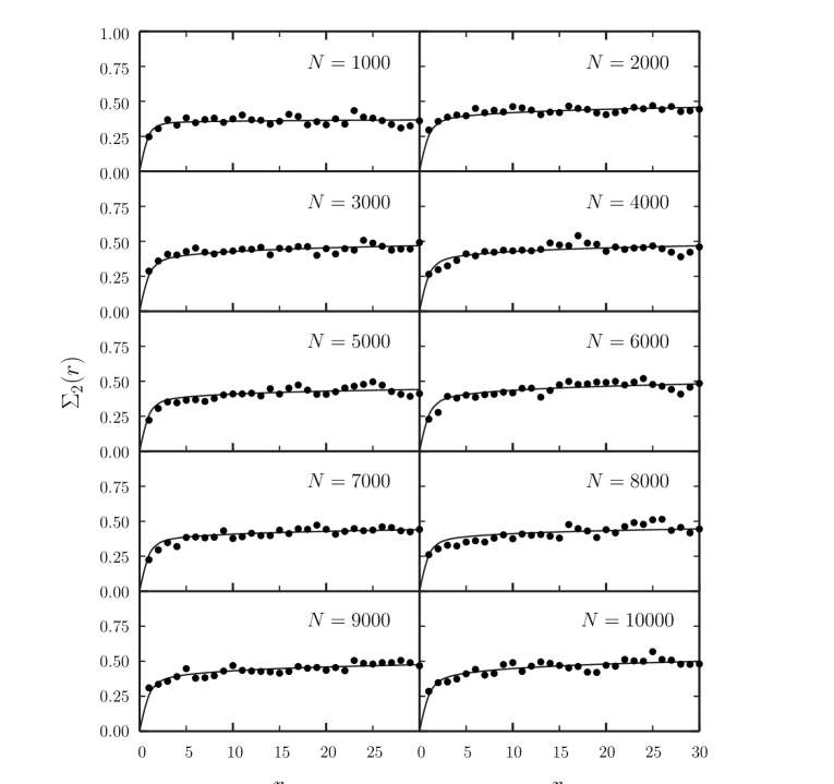
Figure 4: Level number variance $\Sigma_{2}(r)$ for the first 1000, 2000, …, 10000 levels of the irrational oscillator of Eq. (1) with $\alpha=1/\sqrt{2}$ fitted to Eq. (4).

We have fixed the values of the two parameters $A$ = 0.34 and $B$ =1.4 and allowed the third parameter $C$ to vary with the size $N$ of the spectra. The variation of $C$ with $N$ is shown in Fig. 5 and is consistent with the variation observed in Fig. 3 for the width $w$ of the level-spacing distribution.

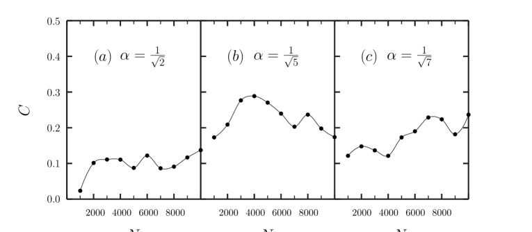
Figure 5: Dependence of the parameter $C$ of Eq. (4) for the level number variance $\Sigma_{2}(r)$ on the size of the spectra, in which $A$ = 0.34 and $B$ =1.4 for $\alpha=1/\sqrt{2}$, $1/\sqrt{5}$, and $1/\sqrt{7}$.

3 Transition to Poisson statistics

In this section, we consider the transition of the spectrum from the harmonic behavior described above to the Poisson statistics. Berry and Tabor [5] considered the level-spacing distribution of a particle in a two-dimensional square-well potential has a Poisson distribution. One can think of several potentials that interpolate between the harmonic oscillator and the square well. The mere existence of such interpolating potentials suggests the possibility of a gradual transition from the harmonic picket-fence shaped spectra to the spectra described by the Poisson statistics.

3.1 Model spectrum

As an example, one may consider the two-dimensional potential

$$V(x,y)=V_{0}\left[\left|\frac{x}{a}\right|^{\frac{2}{{(1-\gamma)}}}+\left|\frac{y}{b}\right|^{\frac{2}{{(1-\gamma)}}}\right],\$$ (5)

which is a harmonic-oscillator potential if $\gamma$ = 0 and a square well if $\gamma$ =1. This potential is a sum of two components, one depending on the variable $x$, and the other depending on $y$. The corresponding Schrödinger equation in cartesian coordinates allows the separation of variables. The eigenvalues are, therefore, given by a sum of the eigenvalues of the two components of the potential

$$E(n,m)=E_{1}(a,n)+E_{1}(b,m).\$$ (6)

Our purpose is to perform a statistical analysis of the spectra which involves mainly large quantum numbers. We can safely apply the WKB approximation and write

$$\int_{-t}^{t}dx\sqrt{\frac{2\mu}{\hbar^{2}}\left[E_{1}(a,n)-V_{0}\left|\frac{x}{a}\right|^{\frac{2}{{(1-\gamma)}}}\right]}=\left(n+\frac{1}{2}\right)\pi,\$$ (7)

where $\pm t$ are the turning points, with

$$t=a\left(\frac{E_{1}(a,n)}{V_{0}}\right)^{\frac{1-\gamma}{2}}.\$$ (8)

Carrying out the integration, one obtains

$$E_{1}(a,n)=V_{0}\left[\sqrt{\frac{\pi\hbar^{2}}{2\mu V_{0}a^{2}}}\frac{\Gamma\left(\frac{4-\gamma}{2}\right)}{\Gamma\left(\frac{3-\gamma}{2}\right)}(n+\frac{1}{2})\right]^{\frac{2}{2-\gamma}}.\$$ (9)

It is easy to see that Eq. (9) yields the correct result in the case of a harmonic oscillator potential, for which $\gamma$ = 0 and $V_{0}=\frac{1}{2}m\omega^{2}a^{2}$, as well as in the case of an infinite square well of width $2a$ where $\gamma$ = 1. Substituting Eq. (9) into Eq. (6) yields

$$E(n,m)=E_{0}\left[\left(n+\frac{1}{2}\right)^{\frac{2}{2-\gamma}}+\alpha\left(m+\frac{1}{2}\right)^{\frac{2}{2-\gamma}}\right],\$$ (10)

where $E_{0}=V_{0}\left[\sqrt{\frac{\pi\hbar^{2}}{2\mu V_{0}a^{2}}}\frac{\Gamma\left(\frac{4-\gamma}{2}\right)}{\Gamma\left(\frac{3-\gamma}{2}\right)}\right]^{\frac{2}{2-\gamma}}\$ and $\alpha=\left(\frac{a}{b}\right)^{\frac{2}{2-\gamma}}.\$

3.2 A model for the transition from the harmonic statistics to the Poissonian

The level spectrum for a system undergoing a crossover transition between two statistics was successfully described in [14, 15, 16] as a superposition of two independent sequences; each one follows one of the two statistics. The model was first proposed by Berry and Robnik [17] to study the transition from the Poisson statistics to that of a Gaussian Orthogonal Ensemble. In this model one has to calculate the gap function for each sub-spectrum

$$E_{i}(s)=\int_{s}^{\infty}dy\int_{y}^{\infty}dxP_{i}(x),\$$ (11)

where $P_{i}(s)$ is level spacing distribution of the sequence $i$. Here we consider a superposition of two sequences. The first is Poissonian, for which

$$E_{1}(s)=e^{-s}.\$$ (12)

The second is harmonic with a spacing distribution represented by Eq. (2), for which

$$E_{2}(s,w) = \frac{1}{2\ {\rm{Erf}}(\frac{1}{w})}\biggl{\{}2+\left(1-s\right){\rm{Erf}}(\frac{1-s}{w})-\left(1+s\right){\rm{Erf}}(\frac{1+s}{w})$$ (13)

$$+\frac{w}{\sqrt{\pi}}\left[e^{-\left(\frac{{\left(1-s\right)}^{2}}{w^{2}}\right)}-e^{-\left(\frac{{\left(1+s\right)}^{2}}{w^{2}}\right)}\right]\biggr{\}}.$$

The transition from a harmonic sequence to a Poissonian is described by a spacing distribution

$$P(s,w,f)=\frac{d^{2}}{ds^{2}}\left[E_{1}((1-f)s)E_{2}(fs,w)\right],\$$ (14)

with $f$ varying from 1 to 0. Substituting Eq. (12) and Eq. (13) into Eq. (14), we finally obtain

$$P(s,w,f)\!\!\!\!\! = \!\!\!\!\!\frac{e^{-(1-f)s}}{2\sqrt{\pi}w{\rm{Erf}}(\frac{1}{w})}\biggl{\{}(1-f)^{2}$$ (15)

$$\!\!\!\!+\frac{1}{2\sqrt{\pi}w}\biggl{[}2e^{-\frac{(1-fs)^{2}}{w^{2}}}[f^{2}-(1-f^{2})w^{2}]+e^{-\frac{(1+fs)^{2}}{w^{2}}}[2f^{2}+(1-f^{2})w^{2}]\biggr{]}$$

$$\!\!\!\!+\frac{1}{2}(1\!\!-\!\!f)\biggl{[}(1\!+\!f\!-\!fs\!+\!f^{2}s){\rm{Erf}}(\frac{1\!\!-\!\!fs}{w})\!+\!(-1\!+\!3f\!\!-\!\!fs\!+\!f^{2}s){\rm{Erf}}(\frac{1\!\!+\!\!fs}{w})\biggr{]}\biggr{\}}.$$

3.3 Numerical Calculation

Numerically, we use Eq. (10) for $\alpha=1/\sqrt{2}$ and different values of the parameter $\gamma$ to calculate the first 10000 energy levels of the potential of Eq. (5). We unfold these spectra using a cubic polynomial and compare the spacing distributions of the unfolded spectra with Eq. (15). The results are shown in Fig. 6 and the best fit values of the mixing parameter $f$ are shown in Fig. 7.

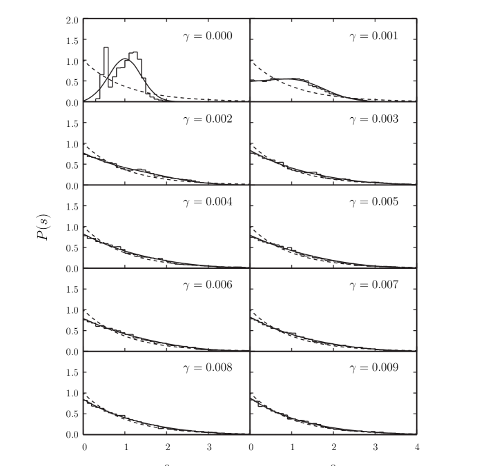
Figure 6: Level spacing distributions for the first 10000 levels of the potential of Eq. (5) with $\alpha=1/\sqrt{2}$, and different values of $\gamma$. The irrational oscillator corresponds to $\gamma$ = 0. The solid and dashed lines represent Eq. (15) and the Poisson distribution respectively.

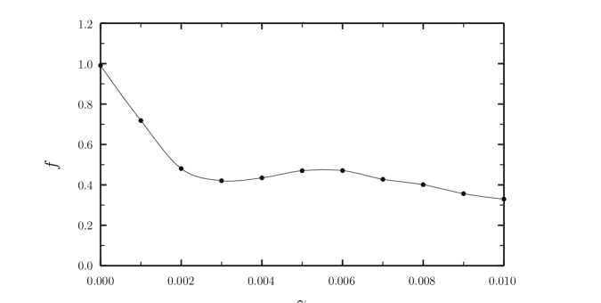
Figure 7: Dependence of the mixing parameter $f$ of Eq. (15), that fits the spacing distribution of the potential of Eq. (5) to the spacing distribution for a superposition of a harmonic and a Poissonian spectra, on the parameter $\gamma$ of the interpolating potential.

4 Analysis of a numerical experiment on a physical system

The harmonic oscillator is a standard model for a large variety of physical systems. It is natural to expect that the non-generic behavior of the spectrum of the harmonic oscillator occurs in real systems.

Carpena et al [13] considered a one-dimensional lattice of large number of sites $(N=2^{17})$ interacting according to a tight-binding hamiltonian. They introduced long range correlations between sites by allowing the power spectral function to decay with exponent $\beta$. If $\beta$ = 0, the sites are uncorrelated and the spectrum has a Poisson statistics. Increasing $\beta$, the level-spacing distribution $P(s)$ acquired new functional forms essentially different from the ones that occur in standard stochastic transitions form Poisson to GOE statistics. They found a critical value of the correlation exponent, $\beta_{cr}$ = 1.55 $\pm$ 0.05, beyond which the Poissonian behavior is lost. As $\beta$ departs from $\beta_{cr}$, the distribution $P(s)$ for small $s$ decreases and simultaneously an increasing peak at $s$ = 1 grows. The spectrum gradually develops a picket-fence behavior. This evolution was also demonstrated by calculating the level-number variance $\Sigma_{2}$ which acquired particularly small values for $\beta>\beta_{cr}$.

We show that the spectra of the disordered system obtained by Carpena et al [13] can be qualified as being in transition from a Poisson statistics to that of a harmonic-oscillator type. For this purpose, we fitted their level-spacing distribution to that of a superposition of a Poissonian and Gaussian functions, which is given by Eq. (15). In Fig. 8, we show the results for the correlated disordered chains with the values of the correlation exponent $\beta$, which have been considered in [13].

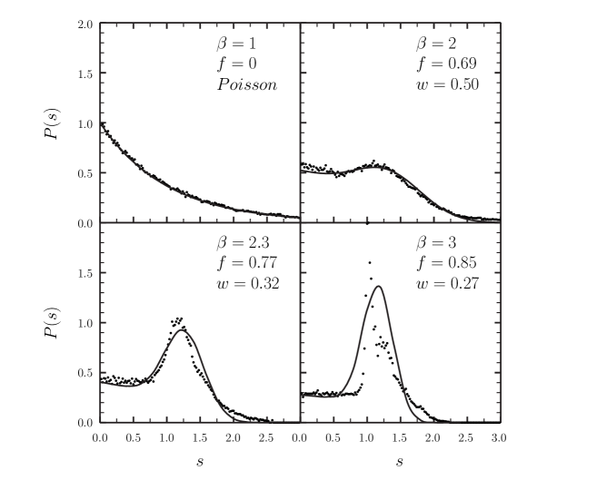
Figure 8: Level-spacing distribution for correlated disordered chains considered in [13] fitted to the distribution in Eq. (15) for a superposition of a Poissonian and an oscillator level sequences.

5 Conclusion

More than a quarter of a century elapsed since Berry and Tabor suggested that the spectra of irrational harmonic oscillators suffer from a strong level repulsion. Most of the subsequent work was based on number theory and showed that the spacing distribution of the two-dimensional oscillator does not converge to a stationary distribution. We have performed a numerical analysis of the level-spacing distributions and level-number variances for irrational oscillators with different frequency ratios. We find that the parameters of these statistics oscillate with increasing the size of the spectra around a mean value that depends on the frequency ratio. We note, however, that the amplitude of the oscillations and the difference between the mean values are small enough to assume the presence of a new “universality class” spectra which we may refer to as the harmonic spectra. We then consider a two-dimensional potential that interpolates between the oscillator and the infinite square well; the latter has a spectrum satisfying the Poisson statistics, and study the transition between the two classes of statistics. We demonstrate that this transition exists in physical systems such as disordered correlated chains.

References

- [1] O. Bohigas, M. J. Giannoni, and C. Schmit, Phys. Rev. Lett. 52, 1 (1984).
- [2] M. L. Mehta, Random Matrix Theory (Academic, San Diego, 1991)
- [3] T. Guhr, A. Müller-Groeling, and H.A. Weidenm ller, Phys. Rep. 299, 189 (1998).
- [4] A. D. Mirlin, Phys. Rep. 326, 259 (2000).
- [5] M. V. Berry and M. Tabor, Proc. R. Soc. London, Ser. A 356, 375 (1977).
- [6] Ya. G. Sinai, Physica A 163, 197 (1990).
- [7] J. Marklof, Comm. Math. Phys. 199, 169 (1998).
- [8] A. Pandey, O. Bohigas, and M. J. Giannoni, J. Phys. A 22, 4083 (1989).
- [9] A. Pandey and R. Ramaswamy, Phys. Rev. A 43, 4237 (1991).
- [10] C. D. Greenman, J. Phys. A 29, 4065 (1996).
- [11] B. Chakrabarti and B. Hu, Phys. Lett. A 315, 93 (2003).
- [12] F. Barra and P. Gaspard, J. Stat. Phys. 101, 283 (2000).
- [13] P. Carpena, P. Bernaola-Galvan and P. Ch. Ivanov, Phys. Rev. Lett. 93, 176804 (2004).
- [14] A. Abd El-Hady, A. Y. Abul-Magd, and M. H. Simbel, J. Phys. A 35, 2361 (2002).
- [15] A. Y. Abul-Magd, C. Dembowski, H. L. Harney, and M. H. Simbel, Phys. Rev. E 65, 056221 (2002).
- [16] A. Y. Abul-Magd and M. H. Simbel, Phys. Rev. E 70, 046218 (2004).
- [17] M. V. Berry and M. Robnik, J. Phys. A 17, 2413 (1984).