Dynamics of a trapped domain wall in a current perpendicular to the plane spin valve nano-structure

Abstract

A study of transverse tail-to-tail magnetic domain walls (DW) in novel current perpendicular to the plane (CPP) spin valves (SV) of various dimensions is presented. For films with dimensions larger than the DW width, we find that DW motion can give rise to a substantial low frequency noise. For dimensions comparable to the DW width, we show that the DW can be controlled by an external field or by a spin momentum torque as opposed to the case of CPP-SV with uniform magnetization. It is shown that in a single domain biased CPP-SV, the spin torque can give rise to 1/f-type noise. The dipolar field, the spin torque and the Oersted field are all accounted for in this work. Our proposed SV requires low current densities to move DW and can simulate devices for logical operation or magnetic sensing without having to switch the magnetization in the free layer.

I Introduction

The study of domain walls (DW) magnetic (static and dynamic) bruno ; molyneux ; hertel ; saitoh and transport berger2 ; zhang ; simanek ; rippard properties have attracted much attention recently due to their relevance for magneto-electronic nano-device applications. In the static case, McMichael and Donahue have shown that in magnetic stripes head-to-head DW can be in vortex or transverse shape mcmicheal . Klaui et al. have observed these DW structures in magnetic thin films and rings klaui .  In this work, we study the dynamics of DW with magnetization mostly restricted to the plane of a nanometer-size thin film.   DW motion can be a source of low frequency noise in magnetic systems and thus hinder any potential applications. Their high frequency behavior can however be tuned by choosing suitable boundary conditions or geometries. Constrained DW oscillations can be high in frequency and hence there is a potential for their use in nano-electronics as resonators rippard .

At least two modes of oscillations have been studied in the literature; a Doring-type oscillation and a Winter mode oscillation doring ; welch ; winter ; thiele . The Doring mode is associated with translations of the center of ’mass’ of the DW in an infinite system, while the Winter modes are non-zero energy modes that, in addition to rigid translation, correspond to propagations along the DW. These modes are found by solving the time-dependent Landau-Lifshitz (LL) equations landau ; malozemoff .

In the following, we focus only on dynamical properties of transverse tail-to-tail DW trapped in stripes with dimensions comparable to their width. This case is proved to be the most interesting due to the unusual magnetization dynamics as opposed to the conventional case of DW with widths being much smaller than the film size. In particular, we find that the low frequency excitations can be reduced in comparison with the usual CPP configuration having a uniform magnetization.   Such uniform magnetization is susceptible to large fluctuations due to spin momentum transfer and gives rise to appreciable $1/f$-like noise. covington We investigate DW formed by pinning the magnetization in the opposite directions at the edges along the easy axis. We show that DW motion can be controlled by a current perpendicular to the plane of the DW magnetization in contrast with the currently actively studied case of DW motion in nano-wires. saitoh

The LL equation is the basis for the present study. Since, we are looking at thermal and current effects, a random field and a spin torque term are also added to the LL equationbrown ; slon ; rebei . We show that in the spin valve (SV) geometry suggested here the spin torque can provide the force needed to move the wall in a controlled fashion with $100$ times smaller current values than those needed to switch the uniform magnetization in a CPP SV.

The paper is organized as follows.  In section II we describe both the theoretical background and the computational model needed for our study. In section III, we discuss the DW structure and we also calculate the lowest eigenmodes of the DW using a simple one dimensional model and compare it to the numerical solution.  It is shown that if the center of the DW is allowed to drift along the easy axis, the contribution to the 1/f-type noise increases.  In section IV, we study the effect of an external field and a CPP current on the SV with and without DW.  We find that SV with a uniform magnetization can be susceptible to unwanted behavior due the spin torque driven instabilities that are absent in a SV with a constrained DW.  We consider a new CPP geometry with a constrained DW between two fixed layers one pinned along and the other pinned perpendicular to the direction of the current flow. We find that in this CPP structure the DW motion can be well controlled with current densities which do not lead to the magnetization instabilities. It is shown that accurate quantification of demagnetizing fields is not essential for a qualitative understanding of the influence of the spin torque on the DW.  In section V, we summarize our results.

II Theoretical Background and Computational Model

For a magnetization $\mathbf{M}$ with magnitude $M_{s}$, the LL equation for $\mathbf{m}=\mathbf{M}/M_{s}$ with a damping in the Gilbert form and time normalized by $\gamma M_{s}$, where $\gamma$ is the gyromagnetic ratio, is given by malozemoff

$$\frac{d\mathbf{m}}{dt}=-\mathbf{m}\times\left(\mathbf{h}^{\mathrm{eff}}+\mathbf{h}_{r}(t)-\alpha\frac{d\mathbf{m}}{dt}\right),$$ (1)

where the effective field $\mathbf{h}^{\mathrm{eff}}$ includes the exchange interaction, the anisotropy field along the $\mathbf{x}$ axis, the demagnetization field, the Oersted field, and the spin torque

$$\mathbf{h}^{\mathrm{eff}}=\frac{2A}{M_{s}^{2}}\nabla^{2}\mathbf{m}-\frac{2K}{M_{s}^{2}}\mathbf{x}(\mathbf{m}\cdot\mathbf{x})+\mathbf{h}_{d}+pI\mathbf{m}\times\mathbf{m}_{p},$$ (2)

The damping term is taken to be $\alpha=0.02$ in the absence of currents and is increased to $\alpha=0.08$ in the presence of spin torques to account for spin accumulation at the normal-ferromagnetic interface. The exchange constant $A=1.6\times 10^{-6}\;\mathrm{erg/cm}$ in this study.  The random field $\mathbf{h}_{r}(t)$ is taken to be uniform and Gaussian white at temperature $T$, $<h_{r,i}(t)h_{r,j}(t^{\prime})>=2\alpha kT/(\gamma M_{s}^{3}V)\delta_{ij}\delta(t-t^{\prime})$. brown  In the presence of spin torques, the white noise assumption foros is strictly valid only for frequencies around the resonant frequency as shown in Ref. rebei, .  Since we are only interested in currents below the critical current, the white noise assumption will not alter the qualitative conclusions of this work.  The size of the discretized cell is taken $2\times 2\;\mathrm{nm}^{2}$ in the plane of the film.  The inclusion of the demagnetizing field is important in DW motion studies and hence a numerical treatment is often needed to get a quantitative understanding of the dynamics of a DW schlomann ; slon2 ; aharoni .  The last term in Eq. 2 is the contribution of a spin torque from the pinned layer (PL) $\mathbf{m}_{B}$.  The prefactor $p$ is dependent of geometrical parameters and $I$ is the current flowing perpendicular to the magnetic multi-layers.  The $p$ prefactor is dependent on the thickness $d$, the cross section $A$ of the layer and the polarization of the current.  Assuming perfect polarization of the conduction electrons, with charge $e$, by the reference layer and neglecting the angular dependence dependence, the spin torque coefficient is given by

$$p=\frac{1}{|e|dAM_{s}^{2}}.$$ (3)

In the following simulations, the anisotropy field is taken $H_{k}=200\;Oe$ and the saturated magnetization is $M_{s}=800.0\;emu/cc$.

III Excitation modes in CPP nano-structures with domain walls

In this section, we introduce the geometry of the DW and study its excitation modes compared to those generated in the uniform case.  We show that the in-plane components of the magnetizations have distinctly different lowest mode frequencies that are directly related to the inhomogeneities of the magnetization due to the DW.  We also discuss the magnetization evolution if we remove the pinning boundary conditions and allow DW to relax to the uniform magnetization state. In addition to the zero temperature dynamics, we investigate the effect of thermal fluctuations on the motion of transverse DW.

III.1 Modes in the case of constrained DW

a
b

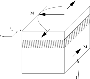
Figure 1: (online color) The CPP-SV magnetic nano-structures consisting of a pinned layer (PL) with fixed magnetization $M_{p}$ and free layer (FL) magnetization $M_{f}$ shown for cases of ( a ) uniform magnetization and ( b) FL with tail-to tail DW. In both cases, the magnetization in the middle of the free layer is perpendicular to the magnetization in the pinned layer.

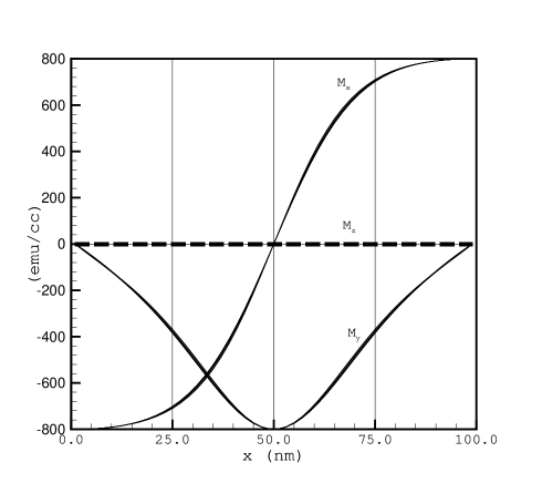
Figure 2: The magnetization distribution for the three components of $\mathbf{M}$ in the DW ($100\times 20\;\mathrm{nm}^{2}$) as a function of coordinate x along the easy x-axis.

Figure 1 shows the geometry of the systems we have studied.  As can be seen from the schematic illustration in Fig. 1 that in contrast with the traditional CPP-SV, we investigate free layer (FL) with inhomogeneous magnetization due to DW in FL coupled to PL with uniform magnetization.  We will add later in section III a third magnetic layer when we discuss the effect of spin torques on the DW. The film has an in-plane easy x-axis along the direction of the magnetization of the bottom pinned layer.  The magnetization of the PL is taken homogeneous.  Fig. 2 shows the magnetization profile for the case of a small current density with DW formed in the plane of FL due to the uniform pinning at the x=$\pm$ L/2 boundaries, where $L$ is the length of the side along the easy axis.

Figure 3 shows the power spectral density (PSD) $|M_{i}(\omega)|^{2}$ of the FL magnetization which has a peak at around $9.0\;\mathrm{GHz}$.  Before calculating the PSD, we first average $\mathbf{M}(x,y)$ over space.  The size of the FL film is taken to be $100\times 20\times 2\;\mathrm{nm}^{3}$ while that of the FL is $100\times 20\times 9\;\mathrm{nm}^{3}$.  For the unpinned boundary case, the average magnetization points along the easy x-axis and the transverse components are oscillating with a frequency approximately twice the ferro-magnetic resonance (FMR) frequency of an infinite thin film given by the Kittel formula, $\omega=\gamma\left(H_{k}\left(H_{k}+4\pi M_{s}\right)\right)^{1/2}$, i.e., around $4.1\;\mathrm{GHz}$.  Figure 3 shows that a film-size of $1000\times 1000\times 3\;\mathrm{nm}^{2}$ has practically the same FMR peak as that of an infinite thin plate.  Thus, the presence of boundaries is an important factor which will be discussed throughout the rest of the paper.

a
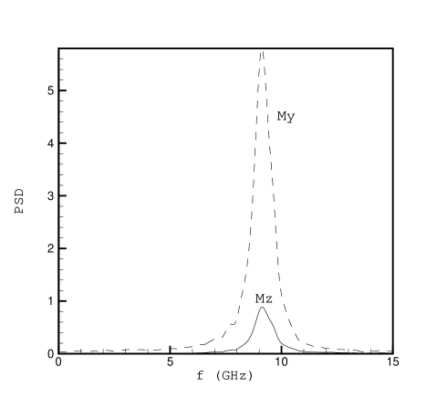
b

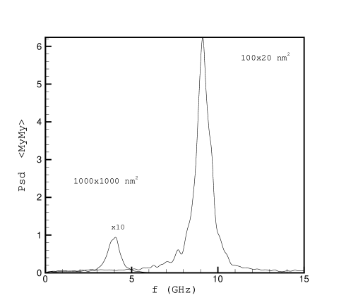
Figure 3: Spectral densities of the uniform magnetization (arbitrary units) in (a) $100\times 20$ $\mathrm{nm}^{2}$ and (b) $1000\times 100$ $\mathrm{nm}^{2}$ thin films as a function of the frequency (no DW). The magnetization is $M_{s}=800\;\mathrm{emu/cc}$ and the anisotropy is $H_{K}=200\;\mathrm{Oe}$ along the easy x-axis. The fluctuations of the $M_{x}$ component are small and do not show up on the scale adopted here.

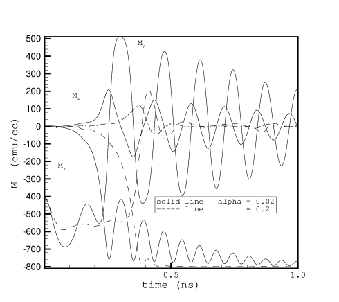
Figure 5: Relaxation of the DW to the uniform state as a function of damping for $\alpha=0.02$ and $\alpha=0.2$.

First we start discussing the DW relaxation as we remove boundary pinning. This relaxation process reflects intrinsic DW modes.  Figure 4 shows the relaxation of the DW when the pinning at the edges is removed at $t=0\;\mathrm{ns}$.  The average x and z components stay zero for more than $0.1\;\mathrm{ns}$ after turning off the pinning.  Afterward, the x-component converges to $M_{s}$ and the z-component begins oscillating around zero.  The y-component starts oscillating immediately around a non-zero average after the removal of the pinning at the edges and after $0.1\;\mathrm{ns}$ starts oscillating instead around zero.  The initial phase of this decay of the DW to the uniform state shows interesting features.  The x-component shows a compression-decompression mode which represents oscillations of the DW around the center and along the easy x-axis (see Fig. 4b-c).  Simultaneously, the y-component shows a behavior similar to a breathing mode.  Finally the last plot shows how a uniform magnetization which is initially along the hard axis relaxes to the state along the easy axis.  Figure 5 shows that large damping makes the DW more stable to external perturbations.

Figure 4: Transient dynamics from the DW state to the uniform magnetization state with thermal fluctuations included: (a) magnetization components a a function of time when pinning has been turned off at $t=0\;\mathrm{ns}$. (b) shows the profile of the $M_{x}$ component at different time steps $1,16,33,50$ and $60$ in units of $\Delta t=0.05$ ns.  (c) same as in (b)but for the $M_{y}$ component. (d) Relaxation of the uniform magnetization from the hard axis position to the easy axis position compared to that of the case of the DW. The damping constant is $\alpha=0.02$. The width of the curves in (b) and (c) represent variations in the y direction at a given point along the x-axis.(this figure can be obtained from one of the authors directly:arebei@mailaps.org or check the published version in Phys. Rev. B June issue 2006)

Magnetization dynamics of the DW can be characterized in terms of its normal modes. In  Fig. 6 we show the spectral densities of the different components of the magnetization found in the DW configuration.  In this case, the x component has a peak at lower frequency than the y-component.  This higher frequency is directly due to the boundary conditions on the magnetization.  The dependency of the magnetization on the y coordinate appears to be very weak.  As a function of the position x, the x and z components have a configuration which is odd under reflection with respect to the center, while the y component configuration is even.

These different excitations of the DW can be qualitatively understood in a 1-D calculation with a simple approximation for the demagnetization field that of an infinite thin film.  If we take, $\mathbf{m}=\left(\sin\theta\cos\varphi,\sin\theta\sin\varphi,\cos\theta\right)$, then the equations of motion for the angular variables are given by

$$\frac{d\theta}{dt}=h_{y}^{\mathrm{eff}}\cos\varphi-h_{x}^{\mathrm{eff}}\sin\varphi-\alpha\sin\theta\frac{d\varphi}{dt},$$ (4)

$$\sin\theta\frac{d\varphi}{dt}=h_{z}^{\mathrm{eff}}\sin\theta-\cos\theta\left(h_{x}^{\mathrm{eff}}\cos\varphi+h_{y}^{\mathrm{eff}}\sin\varphi\right)+\alpha\frac{d\theta}{dt}.$$ (5)

We are looking for excitations around the ground state.  If we take the magnetization to be in-plane, i.e, $\theta_{0}=\frac{\pi}{2}$, and depends only on the x-coordinate, we find that the static solution should satisfy the Sine-Gordon equation

$$\frac{d^{2}\varphi_{0}(x)}{dx^{2}}+\frac{1}{\lambda^{2}}\sin\left[2\varphi_{0}(x)\right]=0,$$ (6)

with the boundary condition $\varphi_{0}\left(-L/2\right)=\pi$ at the left edge and $\varphi_{0}\left(L/2\right)=0$ at the right edge.  $\lambda=\sqrt{2A/K}$ is the width of the DW.  It should be noted here that the same condition arise for DW in infinite films and the only difference is in the boundary conditions.  An analytical solution for this equation does not appear to be possible but it can be found numerically. houston  After linearization, $\theta\rightarrow\theta_{0}+\theta,\;\;\varphi\rightarrow\varphi_{0}+\varphi$, the equations of motion, Eqs. 4 and 5, become

$$\frac{d\theta}{dt} = \frac{2A}{M_{s}^{2}}\frac{d^{2}\varphi(x)}{dx^{2}}+\frac{2K}{M_{s}^{2}}\varphi\cos 2\varphi_{0}-\alpha\frac{d\varphi}{dt},$$ (7)

$$\frac{d\varphi}{dt} = -\frac{2A}{M_{s}^{2}}\frac{d^{2}\theta(x)}{dx^{2}}+G\left(x\right)\theta-\alpha\frac{d\theta}{dt},$$ (8)

where the function $G$ is

$$G(x)=-\frac{2A}{M_{s}^{2}}\left(\frac{\pi}{L}\right)^{2}+4\pi-\frac{2K}{M_{s}^{2}}\cos^{2}\left(\frac{\pi x}{L}\right).$$ (9)

To obtain the function $G$, we have Fourier transformed $\varphi_{0}(x)$ and kept only the first term.  This is sufficient to understand qualitatively the main results of the simulation.

The time-dependent variables $\theta$ and $\varphi$ satisfy homogeneous boundary conditions and represent fluctuations around the equilibrium solution.   If $\varphi(x,t)=\varphi(x)\exp(i\omega t)$, then $\varphi(x)$ can be written in the following form to satisfy the boundary conditions

$$\varphi(x)=\sum_{n=1,3,5,...}a_{n}\cos\left(\frac{n\pi x}{L}\right)+\sum_{m=2,4,6,...}b_{m}\sin\left(\frac{m\pi x}{L}\right),$$ (10)

where $x$ varies in the range $-L/2\leq x\leq L/2$.  The equations of motion then become algebraic equations in $a_{n}$ and $b_{n}$.  Then within a linear approximation, the magnetization components are given by

$$m_{x} = \cos\varphi_{0}(x)-\varphi(x)\sin\varphi_{0}(x),$$ (11)

$$m_{y} = \sin\varphi_{0}(x)+\varphi\cos\varphi_{0}(x).$$ (12)

Since the normal frequencies of the system depend on the wavenumber $n\pi/L$, we see that because of the parity of the ground state $(m_{x}^{0}=\cos\varphi_{0},m_{y}^{0}=\sin\varphi_{0})$, the lowest wavenumber that appears in the y-component is larger $(m=2)$ than that of the x-component $(n=1)$.  This is the reason why the breathing mode has a higher frequency than the spring (or Doring-like mode) mode, Fig. 6-7.  In an infinite plane, the spring mode becomes the Doring mode in our case.  The Doring mode is associated with translation of the DW, i.e., with a zero frequency mode.  In a constrained DW, the pinned edges provide a restoring force and hence the center of the DW will oscillate instead of translating.

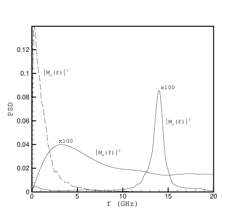
Figure 6: Spectral densities of the magnetization in the constrained DW (arbitrary units). The x component has a peak around, $f=1.0\mathrm{GHz}$. This frequency is that of the Doring-like mode in a finite geometry. The peak of the y-component is at $f=14\;\mathrm{GHz}$ which corresponds to the breathing mode. Both amplitudes for y and z have been multiplied by 100 for better visualization.

a
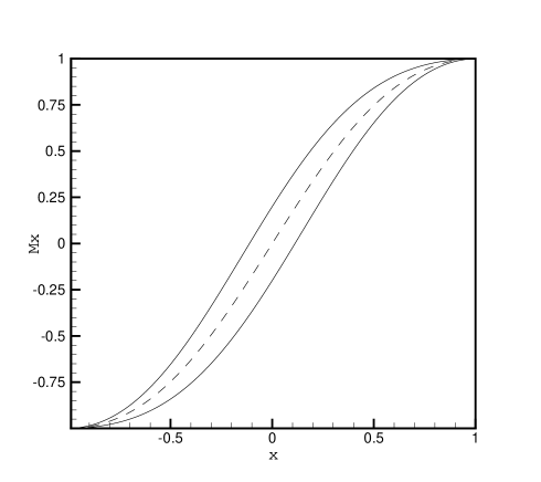
b

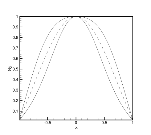
Figure 7: Lowest modes of the DW: The ’spring’ mode (a) and the ’breathing’ mode (b) of the DW. The dashed line is the equilibrium solution. The solid curves represent the amplitudes of the modes around the equilibrium state.  Both $x$ and $M_{x,y}$ have been normalized.

The breathing mode is different from both the Doring and Winter modes.  The Winter modes exist only in in infinite DW as opposed to the constrained DW treated here.  As it can be seen from Fig. 4c and Fig. 7b, the breathing mode is the mode that is mostly excited when the pinned boundary conditions are turned off.

III.2 Low frequency noise due to a drifting domain wall

Finally in this section, we discuss the advantages behind constraining the DW to regions comparable in size to the DW width.   We show that DW motion in large films can be the origin of $1/f$-type noise. This noise has already been suggested from the measurements in Refs. ingvarsson, ; philipp, and is detrimental to any sensing device.

Indeed we find that $1/f$-type noise increases if we increase the size of the thin film so it is much larger than the wall width $\lambda$.  Hence in this case, the center of the DW is allowed to drift away from the middle of the film in either direction along the easy axis due to thermal fluctuations and the demagnetization field.  It has been suggested in many experiments that DW motion can give rise to $1/f$-type noise hardner .  Low frequency noise usually makes structures with non-uniform magnetization undesirable for use in magnetic sensors.  However, the magnetization dynamics pattern changes dramatically if we constrain the DW.  In the following, we first show that making the DW unconstrained does indeed lead to the $1/f$-type noise in general agreement with experimental results ingvarsson ; philipp .

Figure 8: Magnetization Dynamics in the $320\times 20\;\mathrm{nm}^{2}$ elongated CPP valve in the case of $L=320\;\mathrm{nm}\gg\lambda$; $\lambda$ is the DW width :  (a) The average x-component of the magnetization shows dynamics that gives rise to telegraph noise. The DW moves in a thin long strip due to random thermal excitations.  (b) Spectral densities in the x-, -y and z-components of the magnetization in the elongated strip (arbitrary units). Substantial low frequency telegraph type noise is apparent in the x-component. The amplitudes of the y and z peaks have been magnified 100 times.  (c-d) Magnetization distribution in the $xy$-plane at two different times (c) and (d) that correspond to states with positive and negative average $M_{x}$, respectively. This figure can be obtained from the first author or check out the published version in Phys. Rev. B. June 2006.

To observe low frequency behavior in this system we need to reduce the effect of the restoring force on the DW.  This amounts to enlarging the length of the sides along the easy axis of the film to be much larger than the width of the DW.  This way the whole DW can move from the left to the right and back because of thermal fluctuations ( Fig. 8).  Such behavior has been observed in many experiments hardner ; ingvarsson .  Figure 8 shows the PSD’s associated with the different components of the magnetization.  The x-component shows the $1/f$-type behavior as expected.  Figure 8 shows a real-time trace for the average components of the magnetization.  The x-component shows ’switching’-type behavior between two states, a signature of telegraph noise.  The remaining two components are very stable and have much higher frequencies.  The $M_{x}(t)$ behavior of the magnetization resembles the evolution of a two state system (telegraph noise).  It is clear from Fig. 8 that this telegraph noise originates from the DW motion in a shallow double well potential. Finally, it is apparent from Fig. 8 that DW magnetization appears to spend more time closer to the boundary than in the center. This behavior coupled with the telegraph-like noise are indicative of the double well potential for motion in the case of ’unconstrained’ DW. In the case of constricted DW, we do not find this double well potential instead the potential has a single minimum and this is the reason behind the different noise features observed in both cases.  However, it is not obvious what is the origin of such a double well potential and why it disappears in the case of a constricted DW.

In the following we offer a simple explanation for such a behavior. berger  This difference between unconstrained and constrained DW’s can be understood using the notion of charged DW introduced by Neel Neel_dw .  The DW in elongated nano-elements belongs to this category and is characterized by magnetic charges distributed in the vicinity of the DW center as schematically shown in Fig. 9(a).  Moreover because of the finite size of the plate, there are significant boundary charges at either end of opposite sign to that in the DW.  Thus magnetostatic interaction associated with these charges leads to a potential as a function of DW position as shown in Fig. 9(b). The exchange interaction contribution shown in Fig. 9(c) has very strong size dependence due to large exchange energy increase as DW approaches pinned boundaries. Thus, it becomes clear that the total potential for DW motion for unconstrained DW has a double well feature which disappears as the DW gets constrained as shown in Fig. 9(d). In our case the height of the barrier between the two wells is less than $kT$.

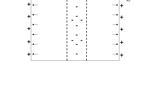
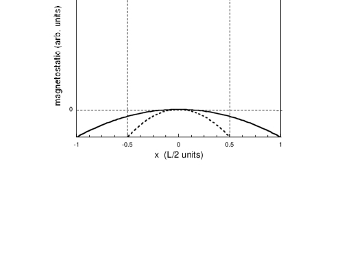
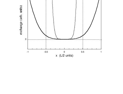
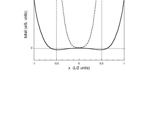
Figure 9: Schematic illustration of a) magnetic charge distribution and contributions to DW potential due to b) corresponding magnetostatic energy c) exchange energy and d) total potential for DW motion along the easy axis. The DW, with width $\lambda_{w}$, is shown to acquire negative charges due to $\nabla\cdot\mathbf{M}$ distributed around DW center and positive charges at the edges. The dashed line is used for the case of constrained DW ($\lambda_{w}$ $\approx$ L) and contrasted with the case of unconstrained DW (solid lines) with $\lambda_{w}$ $<<$ L.

IV Effect of spin torques and Zeeman terms on the DW

In this section we investigate the effect of spin currents and external fields on the magnetization in SV.

First we study a uniformly magnetized SV and calculate the spectral density of the x-component of the magnetization.  We show that the spin torque can be a source of instabilities in this case.  However in the DW case, we show that the effect of the spin torque can be used instead to control its motion.  The CPP structure where this is possible is different than previously proposed structures.  We instead add another magnetic layer to polarize the current in the direction perpendicular to the plane of the SV.

IV.1 Noise in a CPP spin valve with uniformly magnetized layers

Our discussion here will be closely related to the experimental findings in reference covington, where it was shown that spin transfer in a CPP device can give rise to 1/f-type noise. The noise range can be in the GHz regime and in effect makes the use of a CPP device as a GMR sensor unattractive.

In the following we discuss a SV similar to the one treated in Ref. covington, where the magnetization of the free layer is perpendicular to the pinned magnetization. We use a single spin picture to discuss the noise in this system.  We show that this model can reproduce to a great extent the trend in the noise spectrum observed in the experiment in Ref. covington, .  Adopting a single particle picture could be a rather crude approximation in this case rebei ; rebei2 , but it is sufficient for our purpose to demonstrate the contribution of the spin torque to the noise of a CPP device observed in Ref. covington, .  Moreover, the single domain picture discussed here will help us in the interpretation of the numerical results of the more involved case of a DW.

The CPP-SV with uniform magnetization is shown in Fig. 1a.  We take the effective field to be equal to $\mathbf{H}^{\mathrm{eff}}=\left(H_{b}-\nu H_{c},1500,-4\pi M_{z}\right)$ $\mathrm{Oe}$ where the $x$-component is much smaller than the $y$ component.  Therefore in this case the magnetization is expected to be almost perpendicular to the one of the pinned layer.   The saturated magnetization is equal to $1500$ $\mathrm{emu/cc}$.  The AFM field from the pinned layer is assumed small $H_{c}=20\;\mathrm{Oe}$ and the constant $\nu=1$ if the pinned magnetization is along $+x$ and $\nu=-1$  if the pinned magnetization is pointed in the $-x$ direction.  The spin torque term will be represented by an ’effective’ field term $\mathfrak{p}=$ $1000\;\mathrm{Oe}$ which is equivalent to having a $10\;\mathrm{mA}$ fully polarized current flowing into the free layer.  These parameters are chosen to be close to those used in the experiment of reference covington, .  Using similar parameters, figure 10 shows the PSD for the magnetization in a $200\times 100\times 3\;\mathrm{nm}^{3}$ thin film.  This micromagnetic calculation clearly shows that magnetization is almost uniform and is closely aligned with the $1500\;\mathrm{Oe}$ field along the y-axis. Hence we can use a macro-spin picture to calculate the noise spectra in this system.

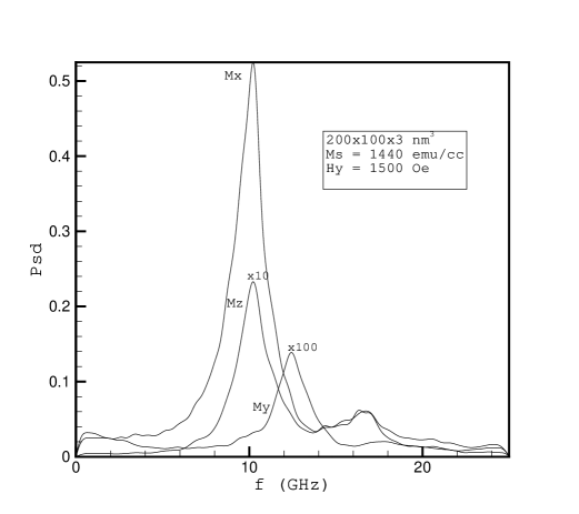
Figure 10: Spectral densities (arbitrary units) of the magnetization in the free layer in the absence of current.

First, we need to determine the equilibrium position in the presence of the spin torque which is not always possible. The spin torque here is comparable to the precession torque from the effective field.  The equilibrium state is found by solving the simultaneous equations

$$M_{x} = r\left(H_{e}-\nu H_{c}\right)$$ (13)

$$M_{y} = r\left(H_{y}-\nu\frac{\mathfrak{p}}{M}M_{z}\right)$$ (14)

$$M_{z} = r\left(-4\pi M_{z}+\nu\frac{\mathfrak{p}}{M}M_{y}\right)$$ (15)

with the constraint $M_{x}^{2}+M_{y}^{2}+M_{z}^{2}=M_{s}^{2}$ and $r$ is a real number to be determined.  These algebraic equations usually have up to four solutions and hence a stability analysis is needed to determine the stable solutions.  This will be part of the PSD calculation of the x-component of the magnetization.  Once, we have found the static solution(s) $\mathbf{M}_{0}$, we make a linear expansion around it, $\mathbf{M}=\mathbf{M}_{0}+\mathbf{m}(t)$, where the perturbation is assumed to have the form $\mathbf{m}(t)=\mathbf{m\exp}\left(-i\omega t\right)$.  The noise is calculated by calculating the susceptibility or the linear response of the magnetization due to an external small ac field $\mathbf{h}(t)$.  This argument neglects the fact that establishing a current across the layers is a non-equilibrium process and that a fluctuation-dissipation argument such as the one used below is not valid in general.  However we have shown in Ref. rebei, that for a system in quasi-equilibrium, deviations from the equilibrium fluctuation dissipation relation are significant only for frequencies far from the FMR frequency of the system.  We assume in the following that the noise in our model depends only on the equilibrium state of the magnetization and hence only the noise around the FMR peak is well described by the method adopted here.

To solve for the small perturbations from equilibrium, we need to solve the following system of equations,

$$\left(i\omega\mathbf{I}+\mathbf{A}\right)\cdot\mathbf{m}=\mathbf{d,}$$ (16)

where the coefficients of the matrix $\mathbf{A}$ are determined from the equations of motion for the magnetization,

$$\mathbf{A}_{11} = \frac{\alpha\gamma}{M_{s}}\left(-H_{y}M_{0,y}+4\pi M_{0,z}^{2}\right),$$

$$\mathbf{A}_{12} = \frac{\alpha\gamma}{M_{s}}\left(2H_{e}M_{0,y}-H_{y}M_{0,x}\right)$$

$$+{\frac{\gamma}{M_{s}}}\left(-2\nu\mathfrak{p}M_{0,y}+4\pi M_{s}M_{0,z}\right),$$

$$\mathbf{A}_{13} = \frac{2\alpha\gamma}{M_{s}}\left(H_{e}M_{0,z}+4\pi M_{0,x}M_{0,z}\right)$$ (17)

$$+{\frac{\gamma}{M_{s}}}\left(-2\nu\mathfrak{p}M_{0,z}+4\pi M_{s}M_{0,y}+H_{y}M_{s}\right),$$

$$d_{1} = -\frac{\alpha\gamma}{M_{s}}\left(M_{0,y}^{2}+M_{0,z}^{2}\right),$$

The remaining coefficients can be determined in a similar way.

The coefficients in front of the x-component of the ac field $\mathbf{h}$(t) are grouped in the vector $\mathbf{d}$.  The stable solutions will be those for which the imaginary part of $\omega$ is negative or zero, $\det\left|i\omega+\mathbf{A}\right|=0.$  In the absence of the spin torque, the frequencies are real in a stable system.  The imaginary frequencies that appear are a signature that the spin torque can act as a (damping) force. The noise spectrum is found by solving for $\mathbf{m}$ in Eq. 16. In the experiment only the noise in x-component, $C_{xx}(\omega)=\int dt\langle M_{x}(t)M_{x}(0)\rangle e^{i\omega t}$ along the pinned magnetization is of interest. It is found from the fluctuation-dissipation relation at inverse temperature $\beta$

$$C_{xx}\left(\omega\right)=\frac{1}{\omega}\mathrm{Coth}\left(\frac{\beta\omega}{2}\right)\operatorname{Im}\frac{\det\left|\begin{array}[c]{ccc}d_{1}&A_{12}&A_{13}\\ d_{2}&i\omega+A_{22}&A_{23}\\ d_{3}&A_{32}&i\omega+A_{33}\end{array}\right|}{\det\left|i\omega+\mathbf{A}\right|}.$$ (18)

These steps are carried out for all the static solutions that are found for each bias field $H_{e}$ in the presence of the spin torque.

The magnetization of the pinned layer is taken in the -x direction (as in the experiment) and the current is positive when it flows from the pinned to the free layer.  In this case we expect to see more noise for negative easy axis fields and less noise for positive easy axis fields.  The $1/f$-type noise is observed when the field along the easy axis is small and negative.  Since this equilibrium analysis can not show actual switching between two states as in the simulations rebei2 and the experiment, we may be able to deduce the switching indirectly since depending on the value of the $H_{e}$ field, we may end up with more than one possible solution to the static equations.  For large negative easy axis fields (Fig. 11), we see the usual shape of FMR curves.  The PSD curves in this section only are normalized differently from those in other sections of the paper.  The damping parameter in this calculation is taken $\alpha=0.005$, which is appropriate for a permalloy even though we expect a higher value due to spin accumulation at the interfaces between a normal conductor and a ferromagnet. rebei

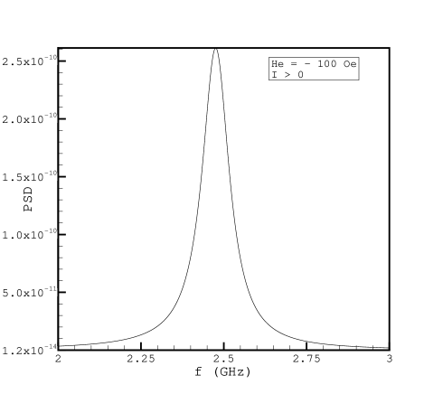
Figure 11: The FMR curve for the free layer with uniform magnetization and for negative bias fields (arbitrary units).

In figure 12, we plot the noise for $H_{e}=100\;\mathrm{Oe}$ and $H_{e}=-100\;\mathrm{Oe}$. Clearly for the case with the positive field, the noise is completely suppressed compared to the case with negative easy axis biasing.  This is consistent with the experiment.  Therefore the state with positive biasing is equivalent to a state with large effective damping.  This large damping is coming from the spin momentum transfer.  If we turn off the current, we get back the usual FMR (bright) spectrum (see Fig. 13) in this case too.  This asymmetry between positive and negative biasing fields close to the perpendicular direction of the free layer will be important later when we have a DW in the presence of spin torques.

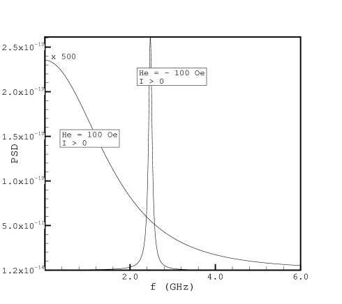
Figure 12: Comparison of the PSD (arbitrary units) for positive and negative biasing fields $H_{e}$.  For $H_{e}=100\;\mathrm{Oe}$ the peak (which is multiplied by $500$) has been completely suppressed and there is a shift to the left, a signature of an over-damped state.

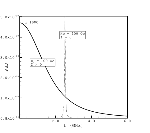
Figure 13: Effect of the spin torque on the PSD (arbitrary units) curve for $H_{e}=100\;\mathrm{Oe}$.  The spin torque is clearly acting as a damping force for positive current.  For $I=0$, the PSD curve has the familiar FMR shape.

Therefore the single spin model captures the ’bright’ and ’dark’ regions of the spectral density for frequencies around the FMR frequency (see Fig. 2 in Ref. covington, ).  Fig. 14a shows the strength of the power as a function of the negative bias field.  Clearly for large biasing we have less noise as expected.  Now, if we plot the same curve for positive fields, Fig. 14b, we find a very interesting result.  For large positive fields, we have the usual ’dark’ regions that reflect high damping states.  As we lower the field, we find that the system now can sustain two states, one bright and one is dark. The dark state is actually less stable than the bright one in this case.  The x-component of the magnetization in the dark state is negative, i.e., opposite to the direction of the easy axis field while the bright one is along the field $H_{e}$.  This is most probably the origin of the $1/f$-type noise in the system.  The $1/f$ region in the experiment appears on the negative side of the easy axis field.  Here it appears on the positive side covington .  The reason is that the zero point of the axis is not well known in the experiment.  The experiment estimates that the magnetization is perpendicular to the pinned layer at $H_{e}=34\;\mathrm{Oe}$ which should correspond to $-20\;\mathrm{Oe}$ in our case.  Therefore there is a shift of about $50\;\mathrm{Oe}$ in the reference point which is approximately the field when two states become possible as a solution to our equations.  The important point we need to remember that the spin system behaves differently for positive and negative bias when there is a spin torque.  This is mainly due to the fact that in one case the spin torque is acting as a regular field, while in the other, it is acting as an extra source of damping.

a
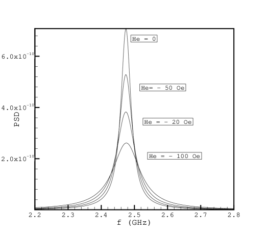
b

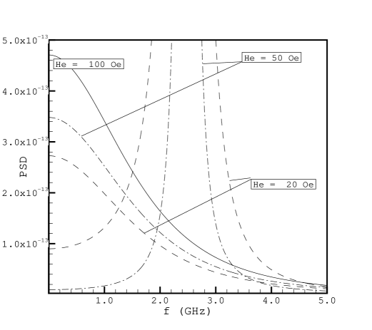
Figure 14: PSD (arbitrary units) for both negative and positive biasing:  (a) PSD (FMR) for negative easy axis biasing fields.  (b) PSD curves for positive bias fields.  For fields approximately between $50\;\mathrm{Oe}$ and $20\;\mathrm{Oe}$, there are two possible states for the system; one is over-damped (dark) and the other is regular (light). Outside this range of fields, only dark or light states exist.

IV.2 Tri-layer CPP structure with a trapped DW

Next, we turn to the study of the DW case. First, we show how a DW in CPP-SV can be manipulated by low currents through the spin torque. The interaction of the DW with an external field will be also shown.

IV.2.1 The effect of spin polarized current

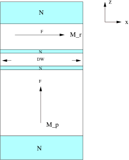
Figure 15: (Online color) Schematic geometry layout for the 3 magnetic -layers CPP structure. The first layer is now polarized along the current direction. The middle has the DW. The third layer has been introduced to enable the GMR sensing of the DW motion.

First, we consider an alternative CPP structure. As will be shown below this modification of the traditional CPP structure can be done for at least three reasons. One reason is to create structures where DW can be manipulated with spin momentum in most efficient way. Secondly, we would like to be able to detect domain wall motion with GMR effect. We also find that the suggested CPP structure modifications may have some advantages in terms of reducing effects of magnetization instabilities due to the spin momentum transfer.  As has been shown, for example in Ref. rebei2, , even in CPP devices with nominally uniform magnetization, the spin torque can give rise to magnetization instabilities. Thus, the latter reason should be kept in mind as an important one.

In the following we consider a CPP structure which has three magnetic layers (Fig. 15) where the DW layer is sandwiched between two pinned magnetic layers with one of them polarized along the direction of the current and the other polarized along the easy axis of the middle DW layer.  In the following simulations, the bottom layer is taken to be $100\times 20\times 9\;\mathrm{nm}^{3}$, the middle layer is $100\times\times 20\times 2\;\mathrm{nm}^{3}$, and the reference layer has the dimensions $100\times 20\times 3\;\mathrm{nm}^{3}$.  In this geometry, the two outer magnetic layers lead to a two different spin torques, $\Gamma=\Gamma_{B}+\Gamma_{T}$, acting on the middle magnetic layer

$$\mathbf{\Gamma}=-pI\left(\mathbf{m}\times\left(\mathbf{m}\times\mathbf{m}_{B}\right)-\mathbf{m}\times\left(\mathbf{m}\times\mathbf{m}_{T}\right)\right),$$ (19)

where $\mathbf{m}_{B}$ ( $\mathbf{m}_{T}$) is the magnetization direction of the bottom (top) layer.  The damping parameter in this section has been increased to $\alpha=0.08$ to better account for spin accumulation rebei .

First, we investigate if the DW can be moved along the easy x-axis with moderate currents.  This will enable a spin torque $\Gamma_{B}=-\mathbf{m}\times\mathbf{h}_{sp}^{B}$ with an effective field along the x-axis and proportional to the y-component of the magnetization in the DW layer that is largest at the center, $\mathbf{h}_{\mathrm{sp}}^{B}=pI(m_{y},-m_{x},0)$.  Since $M_{y}\approx M_{s}$ around $x=0$, this gives us the optimal field needed to push the DW off the center and this appears to be a primary reason why only very low currents are needed to have an appreciable motion of the DW in considered CPP geometry.  Figure 16 shows the effect of the spin torque on the DW in the 3-layer geometry as a function of the current.  We find that the spin torque from the top layer has a relatively small effect on the dynamics of the DW since its effective field is $\mathbf{h}_{\mathrm{sp}}^{T}=pI(0,-m_{z},m_{y})$.  Given that the z-component of the magnetization is practically zero for the currents in the case shown in Fig. 16, the effect of $\mathbf{h}_{\mathrm{sp}}^{T}$ on the magnetization is negligible.  We find that indeed in this geometry, the spin torque can be used to control the motion of DW with very small current densities.  This is primarily due to the fact that the constrained DW has a non-zero y-component of magnetization in the DW region.

The displacement of the DW by the spin torque (we make sure that the Oersted field is not the origin of this motion) is easily understood from the equation of motion without the demagnetization field.  Taking account of only the spin torque, the exchange and the anisotropy, the static equations for the magnetization are

$$\frac{2A}{M_{s}^{2}}\frac{d^{2}m_{x}}{dx^{2}}-\frac{2K}{M_{s}^{2}}m_{x}+pIm_{y} = cm_{x},$$ (20)

$$\frac{2A}{M_{s}^{2}}\frac{d^{2}m_{y}}{dx^{2}}-pI(m_{x}-m_{z}) = cm_{y},$$ (21)

$$\frac{2A}{M_{s}^{2}}\frac{d^{2}m_{z}}{dx^{2}}+pIm_{y} = cm_{z},$$ (22)

where $c(x)$ is a real function and $\mathbf{m}^{2}=1$.  Clearly, in this case the x-component is coupled to the y component which acts as a source term for the x-component.  Neglecting anisotropy and integrating the equation for the $m_{x}$ component around zero, we find that the difference in the slope of $m_{x}$(x) for x=0 and small $x=\epsilon$ is given by

$$\frac{dm_{x}}{dx}|_{x=0}-\frac{dm_{x}}{dx}|_{x=\epsilon}=pI\epsilon m_{y}.$$ (23)

For positive $\epsilon$, i.e. a shift to the right, the slope at $x=0$ is smaller than that at $x=\epsilon$ which is approximately equal to that at $x=0$ in the absence of current.  Therefore $I$ should be negative for positive $m_{y}$ which is approximately equal to the one around $x=0$.  This is confirmed by the numerical integration of LL equation in fig.  16.

a
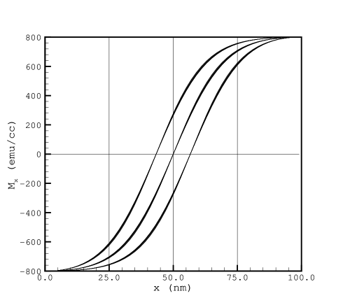
b

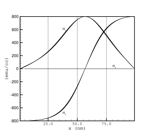
Figure 16: Magnetization profiles of the in-plane components as a function of the sign of the current in the CPP device.  In (a), depending on the sign of the current the curve shifts to the left or to the right. b) The shape of the x and y components of the magnetization in the DW is a slight distortion from that without currents.

The spin torque can therefore be used to move the DW in a controlled fashion with low currents.  In addition we find, that a three-layer structure may actually have lower frequency noise in the presence of spin torque than the structure investigated in Ref. rebei2, .  This potential advantage of our proposed structure is however realized only if the middle layer geometrical dimensions are comparable with the DW width, Fig. 17.  In this case the PSD in the x-component does not show any substantial low frequency noise. For the parameters used here, we find that the DW width is approximately $40$ nm. The dimension of the film is $100$ nm. Therefore the DW is barely constrained and hence the reason behind the sensitivity of the DW to external forces due to fields or currents.

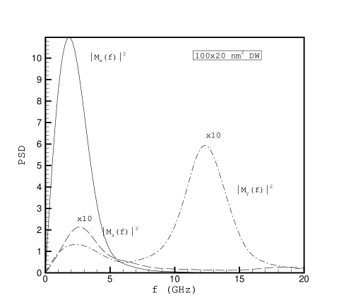
Figure 17: PSD (arbitrary units) of the different components of the magnetization in the presence of current $I=0.001\;\mathrm{mA}$ for a constrained DW.

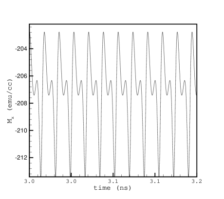
a		b
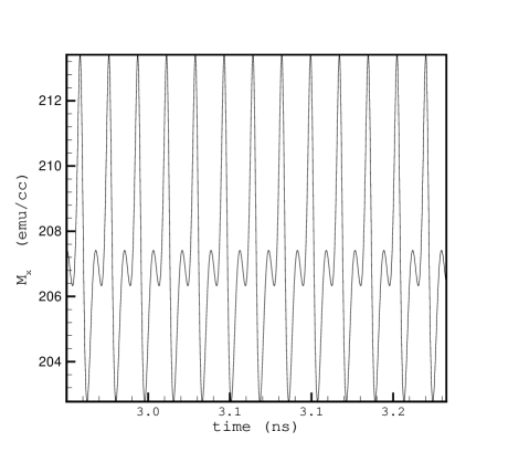
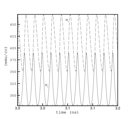
c		d

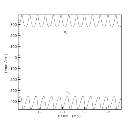
Figure 18: The time evolution of the different components of the average magnetization of the DW for $I=0.1\;\mathrm{mA}.$ (a,c) and $I=-0.1\;\mathrm{mA}$ (b,d). No stationary solutions exist at high currents.

At higher currents, we are no longer in a linear regime.   The numerical integration of the LLG equation shows that the z-component of magnetization becomes more significant as we increase the current and this contributes to the twist of the DW and no stationary solutions are possible in this case.  Figure 18 shows the time evolution of the magnetization for current densities of the order of $1.0\times 10^{7}\;\mathrm{A}/\mathrm{cm}^{2}$.

The magnetization dynamics is a regular periodic rotation.  In this case the spin torque can be used to selectively excite higher modes of the magnetization as compared to those studied in section II.

IV.2.2 The Effect of External Magnetic Field on a DW

Finally in this section, we investigate effect of an external magnetic field. We add a Zeeman term to the total energy and study the displacement of the DW due to an external field along the easy axis.

The external field along the easy axis is applied to the middle layer in the presence of a small current to measure resistance changes across the CPP structure and so that no spin torque effects are appreciable on the DW.  Interestingly the three-layer structure with DW does not require biasing which is needed for standard CPP structures to achieve linear dependence of resistance on the external field.  The calculated transfer curve of resistance $R$ versus field $H$ is shown in Fig. 19. As can be seen this dependence is centered around zero, has a large slope $dR/dH$, and shows small hysteresis.  Moreover, the system appears to be more stable to perturbations by the spin torque and no 1/f-type behavior is observed in this case. Our device is therefore well suited to function as a magnetic sensor. However the proposed structure lacks an important property which is needed in memory applications and that is non-volatility. As we remove the voltage across the CPP-SV, the DW relaxes back to its equilibrium position and hence any state stored in the DW position is lost. Nevertheless, our proposed CPP-SV structure can be incorporated as part of a logic device. Recently, properly redesigned CPP structures have been proposed for reprogammable logic elements ney ; moodera . This latter application does not require non-volatility and hence our device can be utilized in a similar way as in Refs. ney, ; moodera, . Our device has an advantage compared to that proposed in Ref. ney, and that is only much smaller currents are needed in our case.

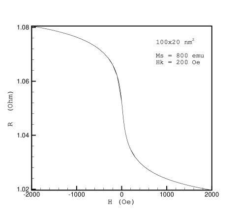
a		b
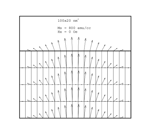
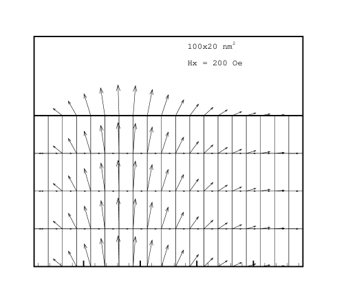
c		d

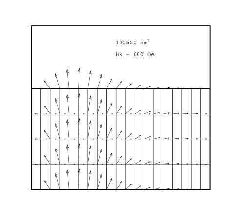
Figure 19: (a) Resistance versus external field applied along the easy x axis for the $100\times 20\;\mathrm{nm}^{2}$ film.  The reference layer is pinned in the $+x$ direction. The resistance is normalized in such a way that for $R=1$ the two layers are parallel and for $R=1.1$ they are anti-parallel.  (b-d) Profiles of the magnetization in the $xy$ plane for zero (b) and positive fields (c-d), respectively.  The scale for the x and y axis are different.  For a given x, five points are plotted along the y-axis.  The DW is fairly uniform along the y axis.

V Summary and Discussion

In summary, we have presented a study of magnetization dynamics for CPP geometry which includes a constrained DW layer.  We have identified a Doring-type mode and a new breathing mode.  It is shown that the lowest modes of the DW dynamics can be understood in terms of the parity of the inhomogeneous ground state. We have investigated in details how the constrained DW dynamics is affected by the spin polarized current and thermal fluctuations and compared it with the traditional single domain free layer structures.  In particular, we found that the currents needed to measure any appreciable motion of the DW are at least two orders of magnitude less than usual values of currents needed to switch the single domain magnetization.  This difference is attributed to the appearance of a significant magnetization component of the constrained DW that is perpendicular to the pinned layer magnetization and the exchange field.

We also find that thermally activated motion of the constricted DW has lower weight in the lower frequency region than that of the unconstrained DW. The latter shows well known telegraph type noise characteristics. This difference can be understood using notion of charged DW introduced by Neel Neel_dw and competition of the magnetostatic and size dependent exchange interaction contributions to the DW potential for motion along the easy axis (see Fig.  9) . The three magnetic layer CPP structure was introduced so that the spin torque effect on DW layer is maximized .  This CPP geometry has been investigated and found to have a number of interesting properties such as (i) DW can be easily controlled by an external field or a polarized current with relatively small current densities; (ii) linear dependence of resistance on the external field and current; (iii) improved magnetization stability characteristics. Experimental realization of the device proposed here requires finding ways to constrain the DW within the middle ’free’ layer. The pinning at the edges can be realized by creating permanent magnets with different coercivity and/or with anti-ferromagnetic (AF) coupling. The AF coupling at the edges needs antiferromagnets with different Neel temperatures ambrose so that a properly designed field-cooling procedure could lead to the pinning in opposite directions at the edges of the magnetic stripe. Other alternatives such as special shaping and padding also have been discussed in the literature in the context of stability of DW in magnetic nano-elements klaui2 .

We thank G. Parker for making his LLG solver available to us.   P. Asselin and W. Scholz have provided us with many helpful comments on the text.   We also acknowledge helpful discussions with T. Ambrose, L. Berger and M. Covington.

References

- (1) P. Bruno, Phys. Rev. Lett. 83, 2425 (1999).
- (2) V. A. Molyneux, V. V. Osipov, and E. V. Ponizovskaya, Phys. Rev. B 65, 184425 (2002).
- (3) R. Hertel, W. Wulfhekel, and J. Kirschner, Phys. Rev. Lett. 93, 257202 (2005).
- (4) E. Saitoh, H. Miyajimi, T. Yamaoka, and G. Tatara, Nature 432, 203 (2004) and references therein.
- (5) L. Berger, J. Magn. Magn. Mater. 162, 155 (1996); Phys. Rev. B 33, 1572 (1986).
- (6) Z. Li and S. Zhang , Phys. Rev. B 70, 024417 (2004).
- (7) E. Simanek and A. Rebei, Phys. Rev. B 71, 172405 (2005).
- (8) W. H. Rippard, M. R. Pufall, S. Kaka, T. J. Silva, and S. E. Russek, Phys. Rev. Lett. 95, 067203 (2005).
- (9) R. D. McMichael and M. J. Donahue, IEEE Trans. Magn. 33, 4167 (1997).
- (10) M. Klaui, H. Ehrke, U. Rudiger, T. Kasama, R. E. Durin-Borkowski, D. Backes, L. J. Heyderman, C. A. F. Vaz, J.A. C. Bland, G. Faini, E. Cambril, and W. Wernsdorfer, Appl. Phys. Lett. 87, 102509 (2005).
- (11) W. Doring, Zeits. f. Naturforschung 3a, 374 (1948).
- (12) A. J. E. Welch, P. F. Nicks, A. Fairweather, and F. F. Roberts, Phys. Rev. 77, 403 (1950).
- (13) J. M. Winter, Phys. Rev. 124, 452 (1961).
- (14) A. A. Thiele, Phys. Rev. B 7, 391 (1973).
- (15) L. Landau and E. Lifshitz, Physik. Zeits. Sowjetunion 8, 153 (1935).
- (16) A. P. Malozemoff and J. C. Slonczewski, Magnetic Domain Walls in Bubble Materials (Academic, New York, 1979).
- (17) M. Covington, M. AlHajDarwish, Y. Ding, N. J. Gokemeijer, and M. A. Seigler, Phys. Rev. B 69, 184406 (2004).
- (18) W. F. Brown, Jr., Phys. Rev. 130, 1677 (1963).
- (19) J. C. Slonczewski, J. Magn. Magn. Mater. 159, L1 (1996).
- (20) A. Rebei and M. Simionato, Phys. Rev. B 71, 174415 (2005).
- (21) J. Foros, A. Brataas, Y. Tserkovnyak, and G. E. W. Bauer, Phys. Rev. Lett. 95, 016601 (2005).
- (22) E. Schlomann, J. Appl. Phys. 43, 3834 (1972).
- (23) J. C. Slonczewski, J. Appl. Phys. 44, 1759 (1973).
- (24) A. Aharoni, J. Appl. Phys. 46, 908 (1975).
- (25) G. Chen, Z. Ding, C-R Hu, W-M Ni, and J. Zhou, Contemporary Math 357, 49 (2004).
- (26) J. B. Philipp, L. Alff, A. Marx, and R. Gross, Phys. Rev. B 66, 224417 (2002).
- (27) S. Ingvarsson, G. Xiao, S. S. P. Parkin, W. J. Gallagher, G. Grinstein, and R. H. Koch, Phys. Rev. Lett. 85, 3289 (2000).
- (28) H. T. Hardner, M. B. Weissman, M. B. Salamon, and S. S. P. Parkin, Phys. Rev. B 48, 16156 (1993).
- (29) L. Berger, private discussion.
- (30) L. Neel, C. R. Acad. Sci. Paris 257, 4092 (1963).
- (31) A. Rebei, L. Berger, R. Chantrell, and M. Covington, J. Appl. Phys. 97, 10E306 (2005).
- (32) A. Ney, C. Pampuch, R. Koch, and K. H. Ploog, Nature 425, 485 (2003).
- (33) J. S. Moodera and P. Leclair, Nature Mat. 2, 707 (2003).
- (34) T. Ambrose, K. Lu, and C. L. Chen, J. Appl. Phys. 85, 6124 (1999).
- (35) M. Klaui, H. Ehrenke, U. Rudiger, T. Kasama, R. E. Durin-Borkowski, D. Bland, G. Faini, E. Gambril, and W. Wernsdorfer, Appl. Phys. Lett. 87, 102509 (2005).