A generalized definition of spin in non-orientable geometries

Abstract

Non-orientable nanostructures are becoming feasable today.  This lead us to the study of spin in these geometries.  Hence a physically sound definition of spin is suggested.  Using our definition, we study the question of the number of different ways to define spin.  We argue that the possibility of having more than one spin structure should be taken into account energetically.  The effect of topology on spin is studied in detail using cohomological arguments.  We generalize the definition of equivalence among (s)pin structures to include non-orientable spaces.

I INTRODUCTION

It has recently been possible to realize new small-size materials with nontrivial topologies.  Tanda et al. were able to have Mobius bands formed by crystals of Niobium and Selenium, $NbSe_{3}$ japan .  Given the recent interest in spintronics, it seems therefore worth the effort to study the possible effect of geometry on spin, especially the combined effect of non-orientability and non-simple connectedness of the space.

Geometric effects in physics are often hidden in terms of constraints.  One good example of this is the $\theta$ vacua of QCD.  Here, the different topological sectors are due to the Gauss constraint ba .  The Chern number also appears due to constraints either in physical space or momentum space.  While studying charge density waves in a torus geometry, Thouless found that in this case, the conductivity is expressed in terms of the Chern number of the manifold and differs from the periodic lattice case in Euclidean space thouless .  Spin currents in semiconductors is still another problem where the Chern number can be used to explain the universality of the spin conductivity in the Rashba model rebei .  In this latter case, the constraint is in momentum space which is homotopic to the plane without the origin, a non-simply connected space.  A final example, we give, is the quantization of the spin of the $SU(2)$ Skyrmion.  The solution to this problem was possible only after extending $SU(2)$ to group $SU(3)$ witten .  However in this extension, a new term is needed in the Lagrangian, the Wess-Zumino term, which has a topological significance and it is related to the disconnectedness of $\mathbf{SO}(3)$.  This latter example shows the inter-connectedness of topology of fields and spin.

In this work, we address similar issues between spin and topology of the physical space of electrons on non-orientable manifolds such as a Mobius band.  In this case there is no global well defined spin structure for the manifold alvarez .  It is well known that quantum mechanical wave functions in non-simply connected spaces can be multivalued and are therefore well defined only on their simply connected covering spaces ba .  For non-orientable manifolds, we show that a definition of spin is possible by going to the orientable double cover of the initial space.  This work was motivated by Tanda’s group and a simple calculation that is presented in the application section.  For thin-film rings, we observed that there is a critical radius at which the trivial (or commonly used) spin representation becomes higher in energy than the non-trivial (twisted) spin representation.  This twisted representation should correspond to the trivial representation on a Mobius band.  The critical radius is estimated to be around $10\;nm$ for a clean conductor.  The typical ring sizes today is in the $100-50\;nm$ range, but it is expected that much smaller sizes will be available in the future saitoh .  Therefore, we claim that at these small scales the spin in the Mobius band and in the ring should ’behave’ the same way, e.g., as it interacts with an external magnetic field or in a ferromagnetic material.  However, before a physical analysis of our claim is possible, a consistent definition of spin structures in non-orientable manifolds is needed.

Spin is an inherently relativistic effect of the electron and follows from requiring Lorentz-invariance of the Schrodinger equation dirac .  The relativistic treatment of the spin is not necessary but it considerably simplifies the formal discussion.

In this paper, we study in some detail, the different spin structures that are possible in non-trivial geometries.  For non-orientable manifolds, the spin group is extended to a pin group where parity is violated similar to the extension of the special rotation group $\mathbf{SO}(3)$ to the full rotation group $\mathbf{O}(3)$.  In this latter case, the $\mathbf{Pin}(3)$ group double covers $\mathbf{O}(3)$ with the group $\mathbf{Spin}(3)$ being a connected component of $\mathbf{Pin}(3)$ which double covers the connected component of $\mathbf{O}(3)$, i.e., $\mathbf{SO}(3)$.  So far only Ref. petry makes use of pin structures to give a viable alternative explanation of a physical theory such as superconductivity.  In this latter work, cooper pairs can be substituted for a more geometrical interpretation which is the existence of a two-inequivalent spin structures in a ring.  Hence in any non-trivial geometry, knowing the number of inequivalent pin structures is important to know before writing a Lagrangian for the dynamics shulman2 .

For the sake of generality, we will allow even time non-orientable manifolds to be part of the discussion.  The work in the literature that covers questions related to the existence and the counting of the different Pin structures is mostly recent.  A comprehensive introduction to Pin group structures can be found in Refs. dabrowski and cecile .

Pin groups first appeared in Ref.atiyah and were derived from Clifford algebras in relation to the K-theory of vector bundles.  After that Karoubi karoubi studied the obstructions to these Pin structures within fiber bundles theory and hence was confined to Pin structures that are only derivable from a Clifford algebra.   As is well known, there are eight non-isomorphic Z₂ extensions of the full Lorentz group ebner .  This is a direct consequence of the disconnectedness of the full Lorentz group and hence there is no unique universal two-cover as is the case for the special orthocronous Lorentz group.

The paper is organized as follows. In section II, we review the results on the orientable case and set the notation for the rest of the paper. In section III we introduce the Pin group through the Clifford algebra. In section IV we introduce a new definition for equivalence among Pin structures that works in non-orientable spaces and study its meaning on the level of representations of the Pinor field. Section V addresses the question of the counting of the inequivalent Pin structures defined on a non-orientable manifold in light of the new definition.  In section VI, we apply the results to two cases; a nano-circuit that has the geometry of a torus and a non-orientable de Sitter space. For the nanocircuit we argue that it is the nontrivial spin representation that must be used instead of the trivial one.  In section VII, we summarize our results.

II SPIN STRUCTURES

In what follows, it is assumed that we are dealing with manifolds with metrics that have the signature $\left(+,-,-,-\right)$ and we will not address any questions that are dependent on the metric propre.  A good review on the mathematics involved here can be found in ref. eguchi .  In this section, we review the spin structures on orientable manifolds and set the notation for the rest of the paper.

For an orientable manifold $\mathcal{\mathbf{B}}$, such as the de Sitter space $\mathbf{R}\times\mathbf{S}^{3}$, a Spin structure exists whenever the second Stiefel-Whitney class vanishes milnor . This is the same as saying that the transition functions of the Lorentzian frame bundle lift up to new transition functions with values in the $\mathbf{Spin}(1,3)$ group. The number of inequivalent Spin structures is given by the number of classes in ${H}^{1}({\mathcal{\mathbf{B}}},\mathbf{Z}_{2})$.  It is well known that $\mathbf{Spin}(1,3)$ is a double cover for the Lorentz group $\mathbf{SO}_{0}(1,3)$, which is the connected component of the identity of the orthogonal group $\mathbf{O}(1,3)$. This double covering induces some restrictions on the transition functions of a Spin structure.

For a manifold to be orientable, the $\mathbf{O}(1,3)$ group structure of the frame bundle should be reducible to $\mathbf{SO}(1,3)$ by choosing an orientation. Since the sequence

$$1\longrightarrow\mathbf{SO}(1,3)\longrightarrow\mathbf{O}(1,3)\longrightarrow\mathbf{Z}_{2}\longrightarrow 1$$ (1)

is a short exact sequence, we get the following long exact sequence hirzb ,

$$0 \longrightarrow H^{0}({\mathcal{\mathbf{B}}},\mathbf{SO}(1,3))\longrightarrow H^{0}({\mathcal{\mathbf{B}}},\mathbf{O}(1,3))\longrightarrow H^{0}({\mathcal{\mathbf{B}}},\mathbf{Z}_{2})$$ (2)

$$\longrightarrow H^{1}({\mathcal{\mathbf{B}}},\mathbf{SO}(1,3))\longrightarrow H^{1}({\mathcal{\mathbf{B}}},\mathbf{O}(1,3))\longrightarrow H^{1}({\mathcal{\mathbf{B}}},\mathbf{Z}_{2}).$$

Recalling that $H^{1}({\mathcal{\mathbf{B}}},\mathbf{SO}(1,3))$ is the set of equivalence classes of Principal $\mathbf{SO}(1,3)$-bundles, then ${\mathcal{\mathbf{B}}}$ is orientable if and only if $\left(iff\right)$ the last map is null. This map is by definition the first Stiefel-Whitney class $\omega_{1}$. Similarly, the short exact sequence

$$1\longrightarrow\mathbf{Z}_{2}\longrightarrow\mathbf{Spin}(1,3)\longrightarrow\mathbf{SO}(1,3)\longrightarrow 1$$ (3)

induces a long exact sequence,

$$...\longrightarrow H^{1}({\mathcal{\mathbf{B}}},\mathbf{Z}_{2})\longrightarrow H^{1}({\mathcal{\mathbf{B}}},\mathbf{Spin}(1,3))\longrightarrow H^{1}({\mathcal{\mathbf{B}}},\mathbf{SO}(1,3))\longrightarrow H^{2}({\mathcal{\mathbf{B}}},\mathbf{Z}_{2}).$$ (4)

Hence ${\mathcal{\mathbf{B}}}$ has a spin structure iff the last map is null. This latter map is the second Stiefel-Whitney class $\omega_{2}({\mathcal{\mathbf{B}}})$ and hence it is the obstruction to a spin structure on the space $\mathbf{B}$.  For non-orientable spaces, $w_{1}\neq 0$, we need to establish similar sequences to the respective groups and this will lead us naturally to the pin group.

III PINOR STRUCTURES

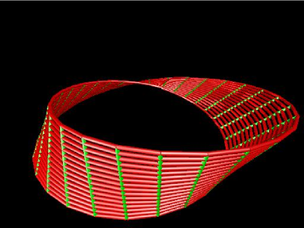
Figure 1: The Mobius band.

Pinor groups are better understood from Clifford algebras atiyah . Given a vector space $\mathcal{V}$ of dimension $n=4$ that is tangent to a point $p\in{\mathcal{\mathbf{B}}}$ and $g(x,y)$ a bilinear non-degenerate quadratic form on $\mathcal{V}$ associated with the metric $(+,-,-,-)$. Let $T(\mathcal{V})=\sum_{i=0}^{\infty}T^{i}(\mathcal{V})$, where

$$T^{i}(\mathcal{V})=\underset{i-times}{\underbrace{\mathcal{V}\times...\times\mathcal{V}}},$$ (5)

is the tensor algebra of $\mathcal{V}$. The set $\mathcal{I}$ generated by the set$\{x\otimes x-g(x,x),x\in\mathcal{V}\}$ is an ideal of $T(\mathcal{V}).$  The quotient space

$$Cl(\mathcal{V},Q)=\frac{T(\mathcal{V})}{\mathcal{I}}$$ (6)

is the Clifford algebra of the vector space $\mathcal{V}$ equipped with the quadratic form $Q(x)=g(x,x).$  Clearly, if $Q(x)=0,Cl(\mathcal{V})$ is simply the Grassmann algebra of forms on $\mathcal{V}$. The dimension of $Cl(\mathcal{V},Q)$ is 2${}^{4}.$  The multiplication in this algebra is induced by the tensor product in $T(\mathcal{V}).$  Let $\left\{e_{0},e_{1},e_{2},e_{3}\right\}$ be an orthonormal basis for $\mathcal{V}$.  Then, the following vectors of $Cl(\mathcal{V},Q)$,

$$e_{0},e_{1},e_{2},e_{3}$$

$$e_{0}e_{1},e_{0}e_{2},e_{0}e_{3},e_{1}e_{2},e_{1}e_{3},e_{2}e_{3}$$

$$e_{0}e_{1}e_{2},e_{0}e_{1}e_{3},e_{0}e_{2}e_{3},e_{1}e_{2}e_{3}$$

$$e_{0}e_{1}e_{3},1$$

form a basis for the algebra.  Moreover, since

$$Q(e_{\mu}+e_{\nu}) = (e_{\mu}+e_{\nu})\otimes(e_{\mu}+e_{\nu})$$ (7)

$$= e_{\mu}\otimes e_{\mu}+e_{\mu}\otimes e_{\nu}+e_{\nu}\otimes e_{\mu}+e_{\nu}\otimes e_{\nu},$$

we have, on the level of algebra,

$$e_{\mu}e_{\nu}+e_{\nu}e_{\mu} = 0\qquad\text{\ \ \ \ \ \ \ if }\mu\neq\nu$$

$$\ e_{\mu}^{2} = 2e^{\mu}e_{\mu}\qquad\mu=0,1,2,3.$$ (8)

Clearly Dirac $\gamma_{\mu}$ matrices form a representation of this algebra ( Majorana representation).  The involution $x\rightarrow-x$ in $\mathcal{V}$ extends naturally to an involution $\alpha$ of the algebra which in turn induces a $\mathbf{Z}_{2}$ grading of $Cl(\mathcal{V},Q)$, i.e.,

$$Cl(\mathcal{V},Q)=Cl^{+}(\mathcal{V},Q)+Cl^{-}(\mathcal{V},Q),$$ (9)

where $Cl^{+}(\mathcal{V},Q)\left(Cl^{-}(\mathcal{V},Q)\right)$ contains the even (odd) elements of the algebra.

A norm function can be defined on $Cl(\mathcal{V},Q)$ by first defining conjugation on the generators:

$$(e_{i_{1}}....e_{i_{p}})^{\ast}=e_{i_{p}}....e_{i_{1}}\>.$$ (10)

Then the norm of $x$ is defined by

$$\left\|x\right\|^{2}=x\alpha(x^{\ast}).$$ (11)

Let $Cl^{\ast}(\mathcal{V},Q)$ be the subset of all invertible elements of $Cl(\mathcal{V},Q).$  Actually in our case where the dimension is even we might as well define the norm without the inversion $\alpha.$  The Clifford group $\Gamma(\mathcal{V},Q)$ is the subgroup of $Cl^{\ast}(\mathcal{V},Q)$  defined by

$$\Gamma(\mathcal{V},Q)=\left\{x\in Cl^{\ast}(\mathcal{V},Q):v\in\mathcal{V},\alpha(x)vx^{-1}\in\mathcal{V}\right\}.$$ (12)

Given $x\in\Gamma(\mathcal{V},Q)$, then it can be represented by an orthogonal transformation

$$\rho(x) : \mathcal{V}\rightarrow\mathcal{V}$$

$$e \rightarrow \alpha(x)ex^{-1}$$ (13)

If we were to drop $\alpha$ from the definition, the map $\rho$ fails to be a representation in the odd dimensional case.  Finally, the Pin group is the subgroup of the Clifford group with elements of modulus one,

$$\mathbf{Pin}(\mathcal{V},Q)=\left\{x\in\Gamma(\mathcal{V},Q):\qquad||x||=1\right\}.$$ (14)

This group doubly covers the orthogonal group $\mathbf{O}(1,3)$. The sequence

$$1\longrightarrow\mathbf{Z}_{2}\longrightarrow\mathbf{Pin}(1,3)\longrightarrow\mathbf{O}(1,3)\longrightarrow 1$$ (15)

is then a short exact sequence. We say that $\mathbf{Pin}(1,3)$ is a $\mathbf{Z}_{2}-$extension of $\mathbf{O}(1,3)$.

Finally, it is important to realize that not all pin groups are derived from a Clifford algebra.  Chamblin chamblin studied the obstructions to non-Cliffordian Pin structures.  Starting from Dabrowski’s semidirect product formula for the Pin group  dabrowski ,  Chamblin found an obstruction to Pin structures through the use of Sheaf cohomology hirzb . The starting short exact sequence that was fundamental to his construction is however not correct.  This is easily seen by applying the second homomorphism theorem. Dabrowski’s formula is

$$\mathbf{Pin}^{a,b,c}(p,q)=\frac{\mathbf{Spin}_{0}(p,q)\odot\mathbf{C}^{a,b,c}}{\mathbf{Z}_{2}},$$ (16)

where $\mathbf{C}^{a,b,c}$ stand for the discrete group of order 8 that is a double covering of the group $\mathbf{G}=\left\{1,T,P,TP\right\}$. The rotation group $\mathbf{O}(p,q)=\mathbf{SO}(p,q)\odot G$ is double covered by the Pin group and there are eight non-isomorphic such groups.  This latter eight is unrelated to the order of the group $\mathbf{C}^{a,b,c}$ . The group $\mathbf{G}$ is isomorphic to $\mathbf{Z}_{2}\otimes\mathbf{Z}_{2}.$ The group $\mathbf{C}^{a,b,c}$ is isomorphic to either of the following groups. The quaternion group $\mathbf{Q}$, the dihedral group $\mathbf{D}_{4}$, the group $\mathbf{Z}_{2}\times\mathbf{Z}_{2}\times\mathbf{Z}_{2}$ and the group $\mathbf{Z}_{2}\times\mathbf{Z}_{4}$. The a, b and c indexes stand for the signs of the squares of the elements of the cover $T,P$ and $PT.$ For example in the quaternion case we can map $i$ to $T$, $j$ to $P$ and $k$ to $TP$. In this case $a=b=c=-$, and so on.  In the rest of the paper, we will be only interested in determining the degrees of freedom on the spin structures for a given topology. We hope to address the question of obstructions in the future.

IV WEAKLY-EQUIVALENT PIN STRUCTURES

In this section, we introduce a new definition for equivalence among (s)pin structures that takes into account the possible non-orientability of the physical space of the system.  The definition is suggested such that the non-orientability is linked to the orientable cover of the space.  This is in analogy with relating non-simply connected spaces to their simply connected covers.

IV.1 Pinor-Frames

Let $\mathcal{\mathbf{B}}$ a manifold with a metric of signature $(+,-,-,-)$ and covered by a simple cover $\left\{U_{i}\right\},\Gamma$ is the $\mathbf{Pin}(1,3)$ group and $\mathbf{G}$ is the orthogonal group $\mathbf{O}(1,3)$. $(\mathcal{\mathcal{\mathbf{P}}},\pi,\mathcal{\mathbf{B}},\mathbf{G})$ is a principal bundle. $(\widetilde{\mathcal{\mathbf{P}}},\widetilde{\pi},\mathcal{\mathbf{B}},\Gamma)$ is the principal bundle induced by the double covering

$$\rho:\Gamma\rightarrow\mathbf{G}\>.$$ (17)

There is a bundle map $\Phi$ between $\widetilde{\mathcal{\mathbf{P}}}$ and $\mathcal{\mathbf{P}}$ such that

$$\Phi\pi = \widetilde{\pi}$$

$$\Phi(\upsilon\cdot\gamma) = \Phi(\upsilon)\Phi(\gamma)$$ (18)

for $\upsilon\in$ $\widetilde{\mathcal{\mathbf{P}}}$ and $\gamma\in\Gamma$ .

Consider now two $\Gamma-$structures $\widetilde{\mathcal{\mathbf{P}}}$ and $\widetilde{\mathcal{\mathbf{P}}^{\prime}}$ over $\mathcal{\mathbf{P}}$ that differ only through an automorphism $\Psi$ of $\Gamma$, in other words, we have a bundle isomorphism $\Theta$ such that

$$\begin{array}[]{llll}\Theta:&\ \widetilde{\mathcal{\mathbf{P}}}&\rightarrow&\ \widetilde{\mathcal{\mathbf{P}}}^{\prime}\\ &\Phi\searrow&&\swarrow\Phi^{\prime}\\ &&\mathcal{\mathbf{P}}&\end{array}$$ (19)

commutes and

$$\Theta(\upsilon\cdot\gamma)=\Theta(\upsilon)\cdot\Psi(\gamma)\text{ \ \ \ \ \ \ }\upsilon\in\widetilde{\mathcal{\mathbf{P}}},\gamma\in\Gamma\>.$$ (20)

$\widetilde{\mathcal{\mathbf{P}}}$ and $\mathcal{\mathbf{P}}$ are said to be weakly-equivalent. Because of the double covering, the map $\Psi$ is involutive.

Next, we state the following definition of a pinor field which is a generalization of the usual spinor field. A Pinor field $\psi$ of type ($\xi,\mathbf{Y})$ on $\mathcal{\mathbf{B}}$ is a section of $\widetilde{\mathcal{\mathbf{P}}}\times_{\Gamma}\mathbf{Y}$  with

$$\xi:\Gamma\rightarrow Hom(\mathbf{Y},\mathbf{Y})$$ (21)

and is a representation map of $\Gamma$ .

Theorem I

The sets of Pinor fields representations in $\widetilde{\mathcal{\mathbf{P}}}$ and $\widetilde{\mathcal{\mathbf{P}}}^{\prime}$ are $\Psi-$ related.

To prove this we first take note of the fact that a section $\sigma$ of $\widetilde{\mathcal{\mathbf{P}}}\times_{\Gamma}Y$  can be represented as a map

$$S : \widetilde{\mathcal{\mathbf{P}}}\rightarrow\mathbf{Y}$$

$$S(\widetilde{u}) = \widetilde{u}^{-1}(\sigma(x))$$ (22)

such that

$$S(\widetilde{u}\cdot\gamma)=\gamma^{-1}\cdot S(\widetilde{u})$$ (23)

Here we have used the fact that an element $\widetilde{u}$ of $\widetilde{\mathcal{\mathbf{P}}}$ represents a map from $\mathbf{Y}$ to $Y_{x}$ . Moreover, the bundle map $\Theta$ can be taken to be the identity map on fibers, i.e.,

$$\Theta\equiv 1:Y_{x}\rightarrow Y_{x}$$ (24)

Let $\left\{\gamma_{ij}\right\}$ and  $\left\{\gamma_{ij}^{\prime}\right\}$ be the transition functions of $\widetilde{\mathcal{\mathbf{P}}}$ and $\widetilde{\mathcal{\mathbf{P}}}^{\prime}$ , respectively. Then it is obvious that the following diagram commutes:

$$\gamma_{ji}:$$

(25)

i.e.,

$$\Psi(\gamma_{ji})=\gamma_{ji}^{\prime}\>.$$ (26)

Therefore given a section $\sigma_{i}:U_{i}\rightarrow\widetilde{\mathcal{\mathbf{P}}}\times_{\Gamma}\mathbf{Y}$, there is a corresponding one $\sigma_{i}^{\prime}~{}:U_{i}\rightarrow\widetilde{\mathcal{\mathbf{P}}}^{\prime}\times_{\Gamma}\mathbf{Y}$ such that

$$\sigma_{i}(x) = [x,y]=[x\cdot\gamma,\gamma^{-1}\cdot y]$$

$$\sigma_{i}^{\prime}(x) = [x,y]=[x\cdot\Psi(\gamma),\Psi(\gamma^{-1})\cdot y]$$ (27)

An element $u$ of $\widetilde{\mathcal{\mathbf{P}}}$ can be represented by an equivalence class $[i,x,\gamma]=[j,x,\gamma_{ji}\gamma]$ with a similar expression for $u^{\prime}$ of $\widetilde{\mathcal{\mathbf{P}}}^{\prime}$ with $\gamma_{ji}$ replaced by $\Psi(\gamma_{ji})$ . This is equivalent to saying that $u$ is a map

$$\mathbf{Y}\rightarrow Y_{x}$$ (28)

with

$$u(y)=\varphi_{i}(x,\gamma\cdot y)\>.$$ (29)

The $\varphi_{i}$’s are the local trivializations of $\widetilde{\mathcal{\mathbf{P}}}$. For the cross sections we have the following diagram

$$\begin{array}[]{ccccc}S:&\widetilde{\mathcal{\mathbf{P}}}&\rightarrow&&\mathbf{Y}\\ \Theta&\downarrow&&\nearrow&S^{\prime}\\ &\widetilde{\mathcal{\mathbf{P}}}^{\prime}&&&\end{array}$$ (30)

so $S(u)=S^{\prime}(\Theta(u))=S^{\prime}(u^{\prime})$. This in turn implies that

$$S^{\prime}(u^{\prime}\cdot\gamma^{\prime}) = \gamma^{{}^{\prime}-1}\cdot S^{\prime}(u^{\prime})$$ (31)

$$= \Psi(\gamma^{-1})\cdot S(u)\>.$$

If $\xi$ is a representation of $\Gamma$ , the above relation trivially extends to

$$S^{\prime}(u^{\prime}\cdot\xi(\gamma^{\prime}))=\Psi(\xi(\gamma^{-1}))\cdot S(u)\>.$$ (32)

We conclude that a pinor field defined on $\mathcal{\mathbf{B}}$ is a quantity independent of the action group within an isomorphism.

IV.2 On frame-Bundles

Let as above $\mathcal{\mathbf{B}}$ be a non-orientable manifold and $\mathcal{\mathbf{B}}^{c}$ its orientable double cover. Here, we propose to treat the question of what happens if the frame bundle $\overline{\mathcal{\mathbf{P}}}$, with group of action taken to be $\mathbf{O}_{+}^{\uparrow}(1,3)$ , is pushed forward with the covering map $p:\mathcal{\mathbf{B}}^{c}\rightarrow\mathcal{\mathbf{B}}$. We take $\{U_{i}\}$ as the cover of $\mathcal{\mathbf{B}}$.

First it should be realized that the transition functions $\overline{g_{ji}}(x^{\prime})$ of $\overline{\mathcal{\mathbf{P}}}$  are the same as those of the tangent bundle $T\mathcal{\mathbf{B}}^{c}$ . By definition, these transition functions are the Jacobian of the transition functions of the coordinate functions:

$$\varphi_{i}^{\prime}:E_{i}\rightarrow V_{i}=p^{-1}(U_{i})\>,$$ (33)

where $E_{i}\subset\mathbf{R^{4}}$ . The transition functions $t_{ji}(x^{\prime})$ of the chart $(V_{i},\varphi_{i})$ are given by

$$t_{ji}^{\prime}=\varphi_{i}^{\prime-1}\varphi_{i}^{\prime}:E_{i}\smallfrown E_{j}\rightarrow E_{i}\smallfrown E_{j}\>.$$ (34)

Therefore the transition functions $a_{ji}(x^{\prime})$ of $T\mathcal{\mathbf{B}}^{c}$ are given by :

$$a_{ji}^{\prime} : V_{i}\smallfrown V_{j}\rightarrow\mathbf{O}_{+}^{\uparrow}(1,3)$$

$$x^{\prime} \longmapsto a_{ji}^{\prime}(x^{\prime})=J(t_{ji}^{\prime})|_{\varphi_{i}^{-1}(x^{\prime})}\>.$$ (35)

Hence we have

$$\overline{g_{ji}}(x^{\prime})\ =a_{ji}^{\prime}(x^{\prime})\>.$$ (36)

This can be easily shown through the coordinate functions.

Now, we describe in more detail the map $p:\mathcal{\mathbf{B}}^{c}$ $\rightarrow\mathcal{\mathbf{B}}$ . The orientable double cover is defined as follows. The Jacobian of the transition functions of $\mathcal{\mathbf{B}}$, $a_{ji}(x)$, that corresponds to $a_{ji}^{\prime}$ in $\mathcal{\mathbf{B}}^{c}$ are defined similarly. From these transition functions, we can form 1-cochains $\theta$

$$\theta_{ij} : U_{i}\smallfrown U_{j}\rightarrow\mathbf{Z}_{2}$$

$$x \longmapsto \theta_{ji}(x)=\det[J(a_{ji})|_{\varphi_{i}^{-1}(x)}].$$ (37)

Therefore to each point $x\in\mathcal{\mathbf{B}}$ , we can associate to it two points $(x,1)$ and $(x,-1)$ where $\pm 1$ is the values of $\theta_{ij}(x)$ . The manifold $\mathcal{\mathbf{B}}^{c}$ is the set of all these points. First we note that $\mathcal{\mathbf{B}}^{c}$ is connected. A curve in $\mathcal{\mathbf{B}}^{c}$ that connects $(x,1)$ to $(x,-1)$ can be given through the unique lifting of a non-orientable closed loop at $x$ spanier . $\mathcal{\mathbf{B}}^{c}$ is also orientable since lifting the $\theta_{ij}$’s will give the determinant of the Jacobian of the $a_{ij}$’s. The manifold $\mathcal{\mathbf{B}}^{c}$ can in fact be interpreted as a bundle structure over $\mathcal{\mathbf{B}}$ with fiber and group $\mathbf{Z}_{2}$ . Diagrammatically we have

$$\overline{\mathcal{\mathbf{P}}}$$

(38)

Therefore for the principal bundle $(\mathcal{\mathbf{B}}^{c},p,\mathcal{\mathbf{B}},\mathbf{Z}_{2})$ the local trivializations are given by

$$\phi_{i}:U_{i}\times\mathbf{Z}_{2}\rightarrow p^{-1}(U_{i})=V_{i}$$ (39)

and the transition functions $g_{ji}(x):\mathbf{Z}_{2}\rightarrow\mathbf{Z}_{2}$ are elements of $\mathbf{Z}_{2}$ , they act as a permutation group of the points that cover $x$ .

Now define a new set $P=\smallsmile_{x\in\mathcal{\mathbf{B}}}P_{x}$ where $P_{x}=\overline{\mathcal{\mathbf{P}}}_{x_{1}^{\prime}}\smallsmile$ $\overline{\mathcal{\mathbf{P}}}_{x_{2}^{\prime}}$ if $p(x_{1}^{\prime})=$ $p(x_{2}^{\prime})=x$ and distinct. We claim that the map

$$p_{\ast} : \mathcal{\mathbf{P}}\rightarrow\mathcal{\mathbf{B}}$$

$$p_{\ast}(u) = x\text{ where }u\in\overline{\mathcal{\mathbf{P}}}\text{ and }p(\overline{\pi}(u))=x$$ (40)

induces a bundle structure on $\mathcal{\mathbf{B}}$. Therefore we expect the following diagram to commute

$$\Lambda:$$

(41)

besides taking fiber to fiber, the map $\Lambda$ should respect the action of the respective groups in both manifolds:

$$\overline{\mathcal{\mathbf{P}}}\times\mathbf{O}_{+}^{\uparrow}(1,3)$$

(42)

$$\Lambda(u\cdot\lambda)=\Lambda(u)\cdot\tau(\lambda)$$ (43)

We would like to find out the group structure $\mathbf{G}$ of this bundle. Assuming that $\mathcal{\mathbf{B}}$ has a metric with signature $(+,-,-,-)$ then the functions $a_{ji}(x)$ defined above are in $\mathbf{O}(1,3)$ . Since $\mathcal{\mathbf{B}}$ is not orientable then $\det a_{ji}(x)=\pm 1$. The elements that cover $x$ differ by an element in $\mathbf{Z_{2}}$ which can be represented by $T$ or $P$ or any other element with determinant -1 and involutive. The first matrix is related to time non-orientability, the second to space non-orientability. These elements describe global actions on the manifold. By construction, the fiber $Y_{x}\simeq\mathbf{O}_{+}^{\uparrow}\smallsmile\mathbf{O}_{+}^{\uparrow}$. So from the above discussion we should expect that the two copies differ by an element of determinant -1. In fact let $a$ be such an element with $a^{2}=1$. Using the map $\mathbf{Z}_{2}\times$ $\mathcal{\mathbf{B}}^{c}\rightarrow\mathcal{\mathbf{B}}$ , a well defined multiplication, then we can write

$$x_{2}^{\prime}=a\cdot x_{1}^{\prime}\>,$$ (44)

where the local coordinates are used , that is

$$x_{1}^{\prime} : V_{i}\rightarrow E_{i}$$

$$x_{2}^{\prime} : V_{j}\rightarrow E_{j}\>.$$ (45)

On the manifold $\mathcal{\mathbf{B}}$ these charts get projected to a single chart around $x$:

$$x_{1}^{\prime} : \text{ \ \ \ }y_{1}:U_{i}\rightarrow E_{i}$$

$$x_{2}^{\prime} : \text{ \ \ \ }y_{2}:U_{j}\rightarrow E_{j}\>.$$ (46)

Therefore, the frames  $u_{1}(x_{1}^{\prime})$ and $u_{2}(x_{2}^{\prime})$ become two frames at the same point $x$. They are related through the transformation $\frac{\partial y_{1}^{\mu}}{\partial y_{1}^{\upsilon}}|_{x}$. But $y_{1}^{\mu}(x)=x_{1}^{\prime\mu}(x)=a_{\epsilon}^{-1}z_{1}^{{}^{\prime}\varepsilon}(x_{2}^{\prime})$ and $y_{2}^{\upsilon}(x)=y_{2}^{{}^{\prime}\upsilon}(x_{2}^{\prime})$, this implies that

$$\frac{\partial y_{1}^{\mu}}{\partial y_{2}^{\nu}}\;=\;\left(a^{-1}\right)_{\epsilon}^{\mu}\;\frac{\partial{z_{2}^{\prime}}^{\epsilon}}{\partial{y_{2}^{\prime}}^{\nu}\;\mid_{x_{2}^{\prime}}}\>.$$ (47)

Since $\frac{\partial z_{2}^{\prime}}{\partial y_{2}^{\prime}}\in\mathbf{O}_{-}^{\uparrow}(1,3)$, we conclude that the transition functions of $\mathcal{\mathbf{P}}$ are in $\mathbf{O}_{+}^{\uparrow}(1,3)\smallsmile a\cdot\mathbf{O}_{+}^{\uparrow}(1,3)$ . There are two possible choices either $a\in\mathbf{O}_{-}^{\uparrow}(1,3)$ or $a\in\mathbf{O}_{-}^{\downarrow}(1,3)$ . Depending on which element $a$ we choose, we end up with different actions on $\mathcal{\mathbf{P}}$ which are equivalent. So the group $\mathbf{G}$ can be either $\mathbf{O}_{+}^{\uparrow}(1,3)\smallsmile$ $\mathbf{O}_{-}^{\uparrow}(1,3)$ or $\mathbf{O}_{+}^{\uparrow}(1,3)\smallsmile$ $\mathbf{O}_{-}^{\downarrow}(1,3)$. Hence, if we have started with $\mathbf{O}_{+}^{\uparrow}(1,3)\smallsmile$ $\mathbf{O}_{+}^{\downarrow}(1,3)$ as the group of symmetry of $\overline{\mathcal{\mathbf{P}}}$ , we would have obtained $\mathbf{O}(1,3)$ as the group of action of $\mathcal{\mathbf{P}}$. On the level of fibers, the map $\Lambda$ is easily seen to be a 2-1 map similar to $p$ by construction.

V WEAKLY-INEQUIVALENT PIN STRUCTURES

In the following , the topological group $\Gamma$ can be taken to be $\mathbf{Pin}(p,q)$ and the group $\mathbf{G}$ the orthogonal group $\mathbf{O}(p,q)$.

Let $(\mathcal{\mathbf{P}}$,$\pi,\mathcal{\mathbf{B}},\mathbf{G})$ be a Principal bundle. Let $\Gamma$ be a double covering for $\mathbf{G}$. Then we have the following exact sequence:

$$1\rightarrow K\rightarrow\Gamma\rightarrow\mathbf{G}\rightarrow 1\>,$$ (48)

where $K=\mathbf{Z}_{2}$. And let

$$\rho:\Gamma\rightarrow\mathbf{G}$$ (49)

be the 2-1 map. We denote by $g_{ji}:U_{i}\cap U_{j}\rightarrow\mathbf{G}$ the transition functions of the bundle $\mathcal{\mathbf{P}}$. The principal bundle $(\widetilde{\mathcal{\mathbf{P}}}$,$\widetilde{\pi},\mathcal{\mathbf{B}},\mathbf{G})$ is called a $\Gamma$ -structure on $\mathcal{\mathbf{P}}$ iff there is a bundle map

$$\Phi : \widetilde{\mathcal{\mathbf{P}}}\rightarrow\mathcal{\mathbf{P}}$$

$$\Phi(\widetilde{u}\cdot\gamma) = \Phi(\widetilde{u})\cdot\rho(\gamma)\>\>\>\>\text{ for }\widetilde{u}\in\widetilde{\mathcal{\mathbf{P}}}\text{\ and }\gamma\in\Gamma$$ (50)

and the functions $g_{ji}$ can be lifted to the transition functions of $\widetilde{\mathcal{\mathbf{P}}}$ , i.e., we have

$$\gamma_{ji}$$

(51)

$$\rho(\gamma_{ji}) = g_{ji}$$

$$\gamma_{ij}\gamma_{kj}^{-1}\gamma_{ki} = 1\>.$$ (52)

The last relation is the cocycle condition. This enables us to define a Ĉech-Cohomology on $\mathcal{\mathbf{B}}$ with coefficients in $\Gamma$:

$$d : C^{1}\longrightarrow C^{2}$$

$$(d\gamma)(ijk) = \gamma_{jk}\gamma_{ik}^{-1}\gamma_{ij}\>.$$ (53)

Hence $\left[\gamma_{ij}\right]\in H^{1}(\mathcal{\mathbf{B}},\Gamma)$ and $\left[g_{ij}\right]\in H^{1}(\mathcal{\mathbf{B}},\mathbf{G}).$ The equivalence class $\left[\gamma_{ij}\right]$ is defined by

$$\left[\gamma_{ij}\right]=\{\gamma_{jk}^{\prime}:\lambda_{i}\gamma_{ij}\lambda_{j}^{-1}\}$$ (54)

with

$$\lambda_{i}:U_{i}\rightarrow\Gamma\>.$$ (55)

It is immediately clear from the above, that $\rho$ induces a map $\rho^{\ast}$ between cohomologies:

$$\rho^{\ast} : H^{1}(\mathcal{\mathbf{B}},\Gamma)\rightarrow H^{1}(\mathcal{\mathbf{B}},\Gamma)$$

$$\rho^{\ast}\left[\gamma_{ij}\right] = [\rho\left[\gamma_{ij}\right]]=\left[g_{ij}\right]\>.$$ (56)

This map is 1-1 and onto if a $\Gamma-$ structure exists.

Now if we assume that the manifold $\mathcal{\mathbf{B}}$ is non-orientable. Then $\mathcal{\mathbf{B}}$ has an orientable double cover $\mathcal{\mathbf{B}}^{c}$. Let {$U_{1}\}$ be a cover for $\mathcal{\mathbf{B}}$ , and

$$\varphi_{i}:E_{i}\rightarrow U_{i}$$ (57)

be the coordinate maps of $\mathcal{\mathbf{B}}$ where $E_{i}\subset R^{n}$. The transition maps $a_{ij}$ are given by

$$a_{ij}:\varphi_{j}\varphi_{i}^{-1}:E_{i}\rightarrow E_{j}\rightarrow E_{i}\rightarrow E_{j}\>.$$ (58)

Now let $x\in U_{i}\smallfrown U_{j}$ and define $\theta_{ij}$ to be the normalized determinant of the Jacobian of the transition functions $a_{ij}:$

$$\theta_{ij} : U_{i}\smallfrown U_{j}\rightarrow\mathbf{Z}_{2}$$

$$\theta_{ij}(x) = \det J[a_{ij}(x)]\>.$$ (59)

Using the properties of the determinant, we can see that $\theta_{ij}$ is a representative of an element of $H^{1}(\mathcal{\mathbf{B}},\mathbf{Z}_{2})$ . We construct $\mathcal{\mathbf{B}}^{c}$ through these cocycles:

$$p:\mathcal{\mathbf{B}}^{c}\rightarrow\mathcal{\mathbf{B}}\>,$$ (60)

where

$$\mathcal{\mathbf{B}}^{c}=\left\{\left(x,\theta_{ij}(x)\right),x\in U_{ij}\right\}\>.$$ (61)

Therefore, $p$ induces a bundle structure. In fact $(\mathcal{\mathbf{B}}^{c},p,\mathcal{\mathbf{B}},\mathbf{Z}_{2})$ is a principal bundle. Note that this fiber bundle is connected if the base space $\mathcal{\mathbf{B}}$ is connected. If $\mathcal{\mathbf{B}}$ were orientable then $\mathcal{\mathbf{B}}^{c}$ would simply be a trivial double covering.

Next, we let $\widetilde{\mathcal{\mathbf{P}}}$ and $\widetilde{\mathcal{\mathbf{P}}}^{\prime}$ be two $\Gamma$-structures on $\mathcal{\mathbf{P}}$ and $\Psi$ is a group isomorphism of $\Gamma$ such that

$$\Psi:$$

(62)

commutes. $\widetilde{\mathcal{\mathbf{P}}}$ and $\widetilde{\mathcal{\mathbf{P}}}^{\prime}$ are said to be weakly equivalent, $\widetilde{\mathcal{\mathbf{P}}}$ $\simeq_{W}\widetilde{\mathcal{\mathbf{P}}}^{\prime}$ , iff we have the following commutative diagram

$$\widetilde{\mathcal{\mathbf{P}}}$$

(63)

and

$$\Theta(\widetilde{u}\cdot\gamma)=\Theta(\widetilde{u})\cdot\Psi(\gamma)\text{ \ \ \ \ \ \ }\widetilde{u}\in\widetilde{\mathcal{\mathbf{P}}},\gamma\in\Gamma\>.$$ (64)

If $\Psi=1,$ we say the equivalence is strong greub .  We believe that weak equivalence is the concept most appropriate from a physical point of view. We have seen above that such fields are $\Psi$-related, moreover this will enable us to concern ourselves only with fields defined on orientable manifolds.  Therefore if we are interested in knowing how many possible physical fields we can have on a given manifold, it is irrelevant how we represent the group of actions on the spinor field as long as they differ by an isomorphism.  We show next that the map $\Psi$ is an involution.  To show this, we observe that the map $\rho$ is a 2-1 map. Let $\gamma^{1}$ and $\gamma^{2}$ the two elements that cover $g$. Since $\rho\Psi(\gamma^{1})=g$ and $\rho(\gamma^{2})=g$, we must either have $\Psi=1$ or

$$\Psi(\gamma^{1}) = \gamma^{2}$$

$$\text{and }\Psi(\gamma^{2}) = \gamma^{1}\>.$$ (65)

The map $\Psi$ acts as a permutation among the couple that cover a given element in $\mathbf{G}$.   Hence the involution follows immediately. A result that follows from the previous statement is that $\Psi|_{K}=1$   .  This is immediate from the fact that $K=\mathbf{Z}_{2}$.

Theorem II

Let $\widetilde{\mathcal{\mathbf{P}}},\widetilde{\mathcal{\mathbf{P}}}^{\prime}$ be $\Gamma$ -structures on $\mathcal{\mathbf{P}}$,

1. Let $\widetilde{\mathcal{\mathbf{P}}}\simeq_{W}\widetilde{\mathcal{\mathbf{P}}}^{\prime}$ . If $\left\{\gamma_{ij}\right\}$ are transition functions for $\widetilde{\mathcal{\mathbf{P}}}$ associated with $\left\{g_{ij}\right\}$ for $\mathcal{\mathbf{P}}$, then $\gamma_{ji}^{\prime}=$ $\Psi\circ\gamma_{ji}$ are transition functions for $\widetilde{\mathcal{\mathbf{P}}}^{\prime}$.

2. If $\widetilde{\mathcal{\mathbf{P}}}$ and $\widetilde{\mathcal{\mathbf{P}}}^{\prime}$ have transition functions $\left\{\gamma_{ij}\right\}$ and $\left\{\gamma_{ij}^{\prime}\right\}$ with $\gamma_{ij}^{\prime}=$ $\Psi\circ\gamma_{ji}$ then $\widetilde{\mathcal{\mathbf{P}}}\simeq_{W}\widetilde{\mathcal{\mathbf{P}}}^{\prime}$.

To show this we observe that:

1. Associated with $\{\gamma_{ij}\}$ is a system $\widetilde{\varphi}_{i}$ of charts

   $$\widetilde{\varphi}_{i} : U_{i}\times\Gamma\rightarrow\widetilde{\mathcal{\mathbf{P}}}\text{, with }$$

   $$\gamma_{ij} : U_{i}\smallfrown U_{j}\rightarrow\mathbf{G}\$$

   $$\text{given by }\widetilde{\varphi}_{i}\widetilde{\varphi}_{j}^{-1}(\widetilde{e}) = \widetilde{e}\cdot\widetilde{\gamma}_{ij}\>.$$ (66)

   Then charts $\widetilde{\varphi}_{i}^{\prime}:$ $U_{i}\times\Gamma\rightarrow\widetilde{\mathcal{\mathbf{P}}}^{\prime}$ defined by $\widetilde{\varphi}_{i}^{\prime}=\Theta\circ\widetilde{\varphi}_{i}$ have transition functions $\gamma_{ij}^{\prime}:U_{i}\cap U_{j}\rightarrow\mathbf{G}$ given by

   $$\gamma_{ij}^{\prime} = \widetilde{\varphi}_{i}\widetilde{\varphi}_{j}^{-1}(\widetilde{e}^{\prime})$$ (67)

   $$= \Theta\circ\widetilde{\varphi}_{i}\circ\widetilde{\varphi}_{j}^{-1}\circ\Theta^{-1}(\widetilde{e}^{\prime})$$

   $$= \Theta[\widetilde{e}\cdot\gamma_{ij}]$$

   $$= \widetilde{e}^{\prime}\cdot\Psi(\gamma_{ij})$$

   $$\Longrightarrow\gamma_{ij}^{\prime}=\Psi(\gamma_{ij})\>.$$ (68)

   That $\left\{\gamma_{ij}^{\prime}\right\}$ satisfy consistency relations and $\rho\circ\gamma_{ij}^{\prime}=g_{ij}$  is immediate.

2. Proof relies here on showing that

   $$\Theta|_{\widetilde{\pi}^{-1}U_{i}}\equiv\widetilde{\varphi}_{i}\widetilde{\varphi}_{i}^{-1}\>,$$ (69)

   is well defined. We set,

   $$\widetilde{\varphi}_{1}^{\prime}(u,1) = e_{1}^{\prime},\>\>\>\widetilde{\varphi}_{1}(u,1)=e_{1}$$ (70)

   $$\widetilde{\varphi}_{2}^{\prime}(u,1) = e_{2}^{\prime}=e_{1}^{\prime}\cdot\gamma^{\prime},\gamma^{\prime}=\pm 1;\text{ \ }\widetilde{\varphi}_{2}(u,1)=e_{2}=e_{1}\cdot\gamma,\gamma=\pm 1$$ (71)

   $$\widetilde{\varphi}_{1}^{\prime}\widetilde{\varphi}_{2}^{\prime-1}(\widetilde{e}_{2}^{\prime})=\widetilde{e}_{2}^{\prime}\cdot\gamma_{12}^{\prime}=\widetilde{e}_{1}^{\prime}\Longrightarrow\gamma_{12}^{\prime}=\gamma.$$ (72)

   Similarly $\gamma_{{}_{12}}=\gamma.$ Then on $\widetilde{\pi}^{-1}\left(U_{i}\smallfrown U_{j}\right)$ , $\Theta$ is well defined if $\widetilde{\varphi}_{1}\widetilde{\varphi}_{1}^{-1}=\widetilde{\varphi}_{2}\widetilde{\varphi}_{2}^{-1}.$

   $$\widetilde{\varphi}_{1}\widetilde{\varphi}_{1}^{-1}(\widetilde{e}_{1}) = \widetilde{e}_{1}$$

   $$\widetilde{\varphi}_{2}\widetilde{\varphi}_{2}^{-1}(e_{1}) = \widetilde{\varphi}_{2}^{\prime}\widetilde{\varphi}_{2}^{-1}\left(\widetilde{e}_{2}\cdot\gamma\right)=\widetilde{\varphi}_{2}^{\prime}(u,\gamma)=\widetilde{e}_{2}^{\prime}\cdot\gamma=\widetilde{e}_{1}^{\prime}\cdot\gamma^{\prime}\gamma$$ (73)

   Finally, $\gamma_{12}=\gamma_{12}^{\prime}$ , since $\Psi$ is an isomorphism :

   $$\Longrightarrow \Psi(1)=1,\Psi(-1)=-1$$ (74)

   $$\Longrightarrow \gamma^{\prime}\gamma=\gamma_{12}^{2}=1,$$ (75)

   which implies that $\Theta$ is well defined.

Hence we proved our statement. Now we try to show that if only weak equivalence is imposed on $\Gamma$-structures on $\mathcal{\mathbf{P}}$, then the number of inequivalent $\Gamma$-structures will no longer be given by $H^{1}(\mathcal{\mathbf{B}},\mathbf{Z}_{2})$ but instead by $H^{1}({\mathcal{\mathbf{B}}}^{c},\mathbf{Z}_{2})$ . Note that the covering induced by $p$ is a regular covering. Hence $p_{\ast}\left(\pi_{1}(\mathcal{\mathbf{B}}^{c},\ast)\right)\lhd\pi_{1}(\mathcal{\mathbf{B}},\ast)$ and this covering is a $\mathbf{Z}_{2}$-covering. We can see right away that the map $\Psi$ has similar properties on the group action level. As an example, take $\mathcal{\mathbf{B}}=RP_{2}$ . Then $\mathcal{\mathbf{B}}^{c}=\mathbf{S}^{2}.$

$$\pi_{1}(\mathcal{\mathbf{B}}) = \mathbf{Z}_{2},$$ (76)

$$\pi_{1}(\mathcal{\mathbf{B}}^{c}) = 1.$$ (77)

The space $\mathcal{\mathbf{B}}$ has in this case two strongly-inequivalent $\mathbf{Pin}^{-}(2)$ structures. If we let $w$ denotes the volume element of the Clifford algebra associated to $\mathbf{Pin}^{-}(3)$, then the two $\mathbf{Pin}^{-}(2)$ structures are obtained through the following coverings

$$\mathbf{Pin}^{-}(3)/\left\{1,\pm w\right\}\rightarrow\mathbf{O}(3)/\left\{1,-1\right\}$$ (78)

If we require only weak equivalence, then both structures become equivalent with

$$\Psi(w) = -w$$ (79)

$$\Psi(1) = 1\>,$$ (80)

and the above two coverings reduce to a single one, namely

$$\mathbf{Pin}^{-}(3)\rightarrow\mathbf{O}(3)\rightarrow\mathbf{S}^{2}\>.$$ (81)

So imposing weak-equivalence is equivalent to factoring out the effect of the non-orientability of the manifold $\mathcal{\mathbf{B}}$. Hence we should expect that $H^{1}(\mathcal{\mathbf{B}}^{c},\mathbf{Z}_{2})$ gives distinct physical $\Gamma$-structures on $\mathcal{\mathbf{B}}$.

Theorem III

$\mathcal{\mathbf{P}}^{c}$ is a $\Gamma$-structure on $\mathcal{\mathbf{P}}$. The induced Principal bundle $p^{-1}\mathcal{\mathbf{P}}\equiv\mathcal{\mathbf{P}}^{c}$  is a trivial double covering for $\mathcal{\mathbf{P}}$. Similarly,  $p^{-1}\widetilde{\mathcal{\mathbf{P}}}\equiv\widetilde{\mathcal{\mathbf{P}}^{c}}$ is a trivial double covering for $\widetilde{\mathcal{\mathbf{P}}}$ and $\widetilde{\mathcal{\mathbf{P}}^{c}}$ is a $\Gamma$-structure on $\mathcal{\mathbf{P}}^{c}$ .

We start first by showing that $\mathcal{\mathbf{P}}^{c}$ is a trivial covering of $\mathcal{\mathbf{P}}$. $\mathcal{\mathbf{P}}^{c}$ is by definition the Principal bundle induced by $p$,

$$F:$$

(82)

Therefore, $\mathcal{\mathbf{P}}^{c}$ and $\mathcal{\mathbf{P}}$ have the same group structure steenrod . Moreover, we have

$$\overline{g}_{ji}(x^{\prime})=g_{ji}\left(p(x^{\prime})\right)\text{ \ \ for }x^{\prime}\in\mathcal{\mathbf{B}}^{c}$$ (83)

The map F is a 2-1 map. Now consider the bundle $\mathcal{\mathbf{P}}\times\mathbf{Z}_{2}$ defined such that

$$\mathcal{\mathbf{P}}\times\mathbf{Z}_{2}$$

(84)

such that

$$p^{\prime}(u,1) = x_{1}^{\prime}$$ (85)

$$p^{\prime}(u,-1) = x_{2}^{\prime}$$ (86)

$$p(x_{1}^{\prime}) = p(x_{2}^{\prime})=x$$ (87)

We claim that $\mathcal{\mathbf{P}}\times\mathbf{Z}_{2}\simeq\mathcal{\mathbf{P}}^{c}$ , i.e., $\Phi$ is a bundle isomorphism. We construct $\Phi$ explicitly. Locally, we have

$$\Phi : \mathcal{\mathbf{P}}\times\mathbf{Z}_{2}\longrightarrow\mathcal{\mathbf{P}}^{c}$$ (88)

$$\left(x,u(x),1\right)\longrightarrow\left(x_{1}^{{}^{\prime}},u\right)$$

$$\left(x,u,-1\right)\longrightarrow\left(x_{2}^{{}^{\prime}},u\right)$$

Therefore, $\overline{\pi}\Phi(x,u,1)=\overline{\pi}($ $x_{1}^{\prime},u)=x_{1}^{\prime}=p^{\prime}(x,u,1)$  and a similar relation holds for $(x,u,1)$. Hence, the above diagram commutes and $\Phi$ carries fibers to fibers. $\Phi$ can then be considered to be a bundle map induced by the identity. A similar diagram for $\widetilde{\mathcal{\mathbf{P}}}$ and $\widetilde{\mathcal{\mathbf{P}}^{c}}$ shows that $\widetilde{\mathcal{\mathbf{P}}^{c}}$ is a trivial double cover of $\widetilde{\mathcal{\mathbf{P}}}$ .

The following diagram gives all possible relations among the transition functions and can be used to prove that $\widetilde{\mathcal{\mathbf{P}}^{c}}$ is a $\Gamma$-structure on $\mathcal{\mathbf{P}}^{c}$.

$$\widetilde{\mathcal{\mathbf{P}}^{c}}$$

(89)

Considering $\mathcal{\mathbf{P}}^{c}$ and $\mathcal{\mathbf{P}}$ as base spaces, the map $\overline{\Phi}$ is induced by $\Phi$. Hence it is a bundle map. We need to check that it is equivariant, i.e.,

$$\overline{\Phi}\left(\widetilde{\overline{u}}\cdot\gamma\right)=\overline{\Phi}(\widetilde{\overline{u}})\cdot\rho(\gamma)\text{ \ \ \ \ \ for all }\gamma\in\Gamma.$$ (90)

We write $\overline{\Phi}$ explicitly. A map that satisfies all the properties of the above diagram is

$$\overline{\Phi}(x^{\prime};\widetilde{\overline{u}})=\Phi(x^{\prime};\widetilde{u}),$$ (91)

where

$$p(x^{\prime})=x$$ (92)

and $\widetilde{\overline{u}}$ ,$\widetilde{u}$ are the same pinor frames. Since multiplication by $\gamma$ leaves the fiber invariant, it is trivially true that $\overline{\Phi}$ is an equivariant map since $\Phi$ is itself equivariant.  Next we define the difference class of two structures. $\widetilde{\mathcal{\mathbf{P}}}$ and $\widetilde{\mathcal{\mathbf{P}}}^{\prime}$ are two $\Gamma$-structures on $\mathcal{\mathbf{P}}$, where the group actions differ by an isomorphism $\Psi$ . The difference class $\delta(\widetilde{\mathcal{\mathbf{P}}},\widetilde{\mathcal{\mathbf{P}}}^{\prime})$ is defined to be

$$\delta_{ji}(x)=\gamma_{ji}(x)\Psi(\gamma_{ji}^{\prime-1}(x)),\text{ \ \ \ \ x}\in U_{ij}\>.$$ (93)

Similarly, we can define $\overline{\delta}$ for the respective double covers. The difference class $\delta(\widetilde{\mathcal{\mathbf{P}}},\widetilde{\mathcal{\mathbf{P}}}^{\prime})$ can be shown to be an element of H${}^{1}(\mathcal{\mathbf{B}},\mathbf{Z}_{2}).$ Similarly, $\overline{\delta}(\widetilde{\mathcal{\mathbf{P}}^{c}},\widetilde{\mathcal{\mathbf{P}}^{c}}^{\prime})$ is an element of H${}^{1}(\mathcal{\mathbf{B}}^{c},\mathbf{Z}_{2}).$  By definition, we have

$$\delta_{ij}(x)=\gamma_{ij}(x)\Psi(\gamma_{ij}^{\prime}(x)^{-1})\>,$$ (94)

and

$$\rho(\gamma_{ij})=\rho(\gamma_{ij}^{\prime})=g_{ij}\>.$$ (95)

This implies that

$$\rho(\delta_{ij}) = 1$$ (96)

$$\Longrightarrow \delta_{ij}(x)\in\mathbf{Z}_{2}$$ (97)

i.e., $\delta_{ij}$ is in the center of $\Gamma$ and

$$(d\delta)(ijk) = \delta_{jk}\delta_{ik}^{-1}\delta_{ij}$$ (98)

$$= \gamma_{ji}\Psi(\gamma_{jk}^{\prime-1})(\gamma_{ik}\Psi(\gamma_{ik}^{\prime-1}))\gamma_{ij}\Psi(\gamma_{ij}^{\prime-1})$$

$$= \gamma_{jk}\Psi(\gamma_{jk}^{\prime-1})(\Psi(\gamma_{ik}^{\prime})\gamma_{ik}^{-1})\gamma_{ji}\Psi(\gamma_{ij}^{\prime-1})$$

$$= \gamma_{jk}(\gamma_{ij}\Psi(\gamma_{ij}^{\prime-1}))\Psi(\gamma_{jk}^{\prime-1})(\Psi(\gamma_{ik}^{\prime})\gamma_{ik}^{-1})\text{ since }\delta_{ij}\in C(\Gamma)$$

$$= \gamma_{jk}\gamma_{ij}\Psi(\gamma_{ij}^{\prime-1}\gamma_{jk}^{\prime-1}\gamma_{ik}^{\prime})\gamma_{ik}^{-1}$$

$$= 1.$$

Hence $\delta_{ij}\in$ $H^{1}(\mathcal{\mathbf{B}},\mathbf{Z}_{2})$ . A similar proof works for $\overline{\delta}_{ij}$.  The difference class can be used to define an equivalence relation among the $\Gamma-$ structures.  In fact, we have $\widetilde{\mathcal{\mathbf{P}}}\simeq_{W}\widetilde{\mathcal{\mathbf{P}}}^{\prime}$ iff $\overline{\delta}(\widetilde{\mathcal{\mathbf{P}}^{c}},\widetilde{\mathcal{\mathbf{P}}^{c}}^{\prime})=1$   .  To show this, suppose that $\widetilde{\mathcal{\mathbf{P}}}$ and $\widetilde{\mathcal{\mathbf{P}}}^{\prime}$ are weakly -equivalent, then

$$\gamma_{ij}(x)=\Psi(\gamma_{ij}^{\prime}(x)),$$ (99)

with  $\Psi^{2}=1$. Moreover we have

$$\overline{\gamma}_{ij}(x) = \gamma_{ij}(p(x^{\prime}))$$ (100)

since

$$\overline{g}_{ij}(x^{\prime})\;=\;g_{ij}(p(x^{\prime})),$$ (101)

which implies that

$$\overline{\gamma}_{ij}(x^{\prime})=\Psi(\overline{\gamma}_{ij}^{\prime}(x)).$$ (102)

Hence the difference class becomes

$$\overline{\delta}_{ij}(x) = \overline{\gamma}_{ij}(x^{\prime})\Psi(\overline{\gamma}_{ij}^{\prime-1}(x^{\prime}))$$ (103)

$$= \overline{\gamma}_{ij}(x^{\prime})(\overline{\gamma}_{ij}^{\prime-1}(x^{\prime}))$$

$$= 1.$$

Now suppose that $\overline{\delta}(\widetilde{\mathcal{\mathbf{P}}^{c}},\widetilde{\mathcal{\mathbf{P}}^{c}}^{\prime})=1$. Hence there exists $\lambda_{i}:p^{-1}(U_{i})\rightarrow\Gamma$ such that

$$d\lambda(ij)=\overline{\delta}(ij)\>.$$ (104)

This is a Čech-coboundary condition, therefore we have

$$\overline{\gamma}_{ij}(x^{\prime})=\lambda_{i}^{-1}(x^{\prime})\Psi(\overline{\gamma}_{ij}^{\prime}(x^{\prime}))\lambda_{j}(x^{\prime})\>.$$ (105)

Now we try to construct locally the bundle isomorphism

$$\Theta:\widetilde{\mathcal{\mathbf{P}}}\rightarrow\widetilde{\mathcal{\mathbf{P}}}^{\prime}$$ (106)

such that

$$\Theta(\widetilde{u}\cdot\gamma) = \Theta(\widetilde{u})\cdot\Psi(\gamma)$$ (107)

and

$$\Phi\circ\Theta = \Phi^{\prime}\;.$$ (108)

First we have the following commutative diagram:

$$\widetilde{\mathcal{\mathbf{P}}^{c}}$$

(109)

It should be clear from this diagram that locally $\Theta$ and $\overline{\Theta}$ are the same. Hence a construction of $\overline{\Theta}$ will immediately give one for $\Theta$ . Let $V_{i}=\widetilde{\overline{\pi}}(p^{-1}(U_{i}))$ and define $\overline{\Theta}$ locally by

$$\overline{\Theta}_{i}:V_{i}\rightarrow\widetilde{\mathcal{\mathbf{P}}^{c}}^{\prime}$$ (110)

$$\widetilde{\overline{u}}\rightarrow\sigma_{i}^{\prime}(\widetilde{\overline{\pi}}(\widetilde{\overline{u}}))\cdot\lambda_{i}\Psi(\gamma_{i}(\widetilde{\overline{u}}))$$ (111)

where $\sigma_{i}^{\prime}$ is a local cross section of $\widetilde{\mathcal{\mathbf{P}}^{c}}^{\prime}$ and $\gamma_{i}$ is an element of $\Gamma$ such that

$$\widetilde{\overline{u}}=\sigma_{i}(\widetilde{\overline{\pi}}(\widetilde{\overline{u}}))\cdot\gamma_{i}(\widetilde{\overline{u}})$$ (112)

If $\gamma\in\Gamma$ , then

$$\overline{\Theta}_{i}(\widetilde{\overline{u}}\cdot\gamma) = \sigma_{i}^{\prime}(\widetilde{\overline{\pi}}(\widetilde{\overline{u}}\cdot\gamma))\cdot\lambda_{i}\Psi(\gamma_{i}(\widetilde{\overline{u}}\cdot\gamma))$$ (113)

$$= \overline{\Theta}_{i}(\widetilde{\overline{u}}).\Psi(\gamma)\>.$$

This map is well defined globally. On intersection $V_{i}\smallfrown V_{j}$

$$\sigma_{i}(\widetilde{\overline{\pi}}(\widetilde{\overline{u}}))\cdot\lambda_{i}\Psi(\gamma_{i}(\widetilde{\overline{u}}) = \sigma_{i}(\widetilde{\overline{\pi}}(\widetilde{\overline{u}}))\gamma_{ji}^{{}^{\prime}}\lambda_{i}\Psi(\gamma_{i})$$ (114)

$$= \sigma_{i}(\widetilde{\overline{\pi}}(\widetilde{\overline{u}}))\lambda_{j}\Psi(\gamma_{ji})\Psi(\gamma_{i})$$

$$= \sigma_{i}(\widetilde{\overline{\pi}}(\widetilde{\overline{u}}))\lambda_{j}\Psi(\gamma_{j}),$$

as it should be.

Theorem IV

Let $\widetilde{\mathcal{\mathbf{P}}}$ be a $\Gamma$-structure on $\mathcal{\mathbf{P}}$. $\widetilde{\mathcal{\mathbf{P}}^{c}}$ is the corresponding double cover. Then for each element $\overline{\zeta}\in H^{1}(\mathcal{\mathbf{B}}^{c},\mathbf{Z}_{2})$ there exist a non weakly-equivalent $\Gamma-structure$ $\widetilde{\mathcal{\mathbf{P}}}^{\prime}.$

Let $\overline{\zeta}_{ij}$ be a representation of $\overline{\zeta}$ and $\Psi$ is an isomorphism as above. Define the following functions:

$$\overline{\gamma}_{ij}(x^{\prime})=\overline{\zeta}_{ij}^{-1}\cdot(\overline{\gamma}_{ij}^{\prime}(x^{\prime}))\>.$$ (115)

They clearly satisfy the cocycle condition and hence they form the transition functions of a principal bundle which we call $(\widetilde{\mathcal{\mathbf{P}}^{c}}^{\prime},\widetilde{\overline{\pi}}^{\prime},\mathcal{\mathbf{B}}^{c},\Gamma)$ . Note also that

$$\overline{\delta}_{ij}=\overline{\gamma}_{ij}(\overline{\gamma}_{ij}^{{}^{\prime}})=\overline{\zeta}_{ij}\;,$$ (116)

and

$$\rho(\overline{\gamma}_{ij})=\rho(\overline{\gamma}_{ij}^{\prime})=\overline{g}_{ij}.$$ (117)

Now, to get the Principal bundle $(\widetilde{\mathcal{\mathbf{P}}^{c}}^{\prime},\widetilde{\overline{\pi}}^{\prime},\mathcal{\mathbf{B}}^{c},\Gamma)$ we use the fact that $(\mathcal{\mathbf{B}}^{c},p,\mathcal{\mathbf{B}},\mathbf{Z}_{2})$ is a Principal bundle with transition $\theta_{ij}(x)\in\mathbf{Z}_{2}$ . Hence the following diagram commutes:

$$\widetilde{\mathcal{\mathbf{P}}^{c}}^{\prime}$$

(118)

Therefore $(\widetilde{\mathcal{\mathbf{P}}^{c}}^{\prime},\widetilde{\overline{\pi}}^{\prime},\mathcal{\mathbf{B}}^{c},\Gamma)$ is a Principal bundle with transition functions

$$\psi_{ij}(x)=\theta_{ij}(x)\cdot\overline{\gamma}_{ij}^{\prime}(x^{\prime})\>.$$ (119)

Here, we have used the trivial extension of $\Gamma$ , i.e.,

$$1\rightarrow\mathbf{Z}_{2}\rightarrow\mathbf{Z}_{2}\otimes\Gamma\rightarrow\Gamma\rightarrow 1\>.$$ (120)

The bundle $\widetilde{\mathcal{\mathbf{P}}}^{\prime}$ is constructed with the same transition functions. Therefore we set

$$\gamma_{ij}^{\prime}(x)=\theta_{ij}(x)\cdot\overline{\gamma}_{ij}^{\prime}(x^{\prime}).$$ (121)

This ends our main section which relates the number of inequivalent pin structures to the first Cohomology group of the associated orientable cover of the underlying non-orientable space.

VI APPLICATIONS

In this last section, we discuss two examples: the first deals with an electron in a nano-circuit.  The second deals with a non-orientable space.

VI.1 Transport in nano-Circuits

In this section, we follow the notation of Negele and Orland negele . The geometry of the circuit is nontrivial; it has a ‘hole’. The homotopy group of the torus is $\pi_{1}\left(T^{2}\right)=\mathbf{Z}\oplus\mathbf{Z}$. It is a two-dimensional surface. However the electrons are not only constrained to the surface, but they can be also inside. Therefore the geometry of the circuit is in fact homeomorphic to $D\times\mathbf{S}^{1}$ where $D$ is a disk in $\mathbb{R}^{2}$, i.e, a simply connected region. Moreover the manifold is orientable in this case and hence the nontrivial spinor is dictated by the circle around the hole (see figure 2).  According to our discussion in previous sections, any non-orientability will be factored out.  Hence, the following discussion will equally apply to a Mobius band.  For this manifold, there are two possibilities to define spinors since $H^{1}\left(\mathbf{M},\mathbf{Z}_{2}\right)=\mathbf{Z}_{2}$. The vector potential that corresponds to the non-trivial one differs by an element in the Cohomology class $\lambda$:petry

$$A_{\mu}\rightarrow A_{\mu}-\frac{i\hbar c}{2e}\lambda^{-1}\partial_{\mu}\lambda,$$ (122)

with

$$\oint\lambda^{-1}\partial_{\mu}\lambda\cdot dx=2\pi i.$$ (123)

The function $\lambda$ can always be chosen to be defined on the unit circle:

$$\lambda:M\rightarrow\text{ \ }U(1)\subset\mathbb{C}$$

Therefore the magnetic flux will change by a discrete value for each closed path traveled by an electron around the circuit

$$\oint\left(A_{\mu}-\frac{i}{2e}\lambda^{-1}\partial_{\mu}\lambda\right)\cdot dx=\oint A_{\mu}\cdot dx^{\mu}+\frac{hc}{2e}$$ (124)

It is interesting to observe that Magnus and Schoenmaker magnus had to postulate the quantization of flux to be able to recover the Landauer-Buttiker formula for the conductivity. In our case the quantization is automatic for the non-trivial spin structure. It will be argued below that for this circuit, it is the configuration with non-trivial spin structure that must be adopted based on energy arguments. The Frohlich-Studer ($FS$) theory frohlich is a non-relativistic theory that explicitly exhibits the spin degrees of freedom. This latter theory is $U(1)\times SU(2)$ gauge-invariant.  The $SU(2)$ symmetry comes from the spin degrees of freedom of the wave function of the electron. For a magnetic field $(\mathbf{A}=\frac{1}{2}\mathcal{\mathbf{B}}\times\mathbf{r})$ and an electric field in the $z$-direction, the covariant derivatives in the $FS$ equation take the form:

$$D_{t}=\partial_{t}+e\varphi-ig\mu S_{z}B$$ (125)

and the spatial derivatives are

$$D_{1} =\partial_{1}-ieA_{1}+i\left(-2g\mu+\frac{e\mu}{2m}\right)ES_{y},$$ (126)

$$D_{2} =\partial_{2}-ieA_{2}+i\left(-2g\mu+\frac{e\mu}{2m}\right)ES_{x},$$

$$D_{3} =\partial_{3}.$$

In two dimensions with $z=x+iy$, they acquire a simple form

$$D_{+}=D_{1}+iD_{2}=\partial_{z}-ieA_{+}+g^{{}^{\prime}}ES_{+},$$ (127)

with

$$A_{+}=\frac{1}{2}iBz,\qquad S_{+}=S_{x}+iS_{y},\qquad g^{\prime}=-2g\mu+\frac{e\mu}{2m}.$$

For a one dimensional ring with radius $a$, $z=ae^{i\phi}$. Hence, we can simply set $x^{2}+y^{2}=a^{2}$ without loosing any essential spin-orbit type terms in the Hamiltonian as it is the case in the standard formulation meijer .

Next we comment on a procedure for obtaining the Green’s function and the effective action for a particle interacting with an electromagnetic field $F_{\mu\nu}=\partial_{\mu}A_{\nu}-\partial_{\nu}A_{\mu}$ based on the proper time method schwinger .  This is a relativistic method that starts with the Dirac equation. We just state the results since they exhibit explicit gauge invariance. For the one-particle Green’s function, we have

$$G\left(x^{\prime},x^{\prime\prime}\right) =i\int_{0}^{\infty}dse^{-im^{2}s}$$ (128)

$$\times\left[-\gamma_{\mu}\left(x(s)^{{}^{\prime}}\left|\Pi_{\mu}(s)\right|x(0)^{{}^{{}^{\prime\prime}}}\right)\right.$$

$$+\left.m\left(\left.x(s)^{{}^{\prime}}\right|x(0)^{{}^{{}^{\prime\prime}}}\right)\right],$$

where

$$\left(\left.x(s)^{{}^{\prime}}\right|x(0)^{{}^{{}^{\prime\prime}}}\right) =-\frac{i}{\left(4\pi\right)^{2}}\exp\left[ie\int_{x"}^{x^{\prime}}dx^{\mu}A_{\mu}(x)\right]$$

$$\frac{1}{s^{2}}e^{-L(s)}\exp\left[i\frac{1}{4}\left(x^{{}^{\prime}}-x^{{}^{\prime\prime}}\right)eF\coth\left(eFs\right)\left(x^{{}^{\prime}}-x^{{}^{\prime\prime}}\right)\right]$$

$$\times\exp\left[i\frac{1}{2}e\sigma Fs\right],$$ (129)

$$\left(x(s)^{{}^{\prime}}\left|\pi_{\mu}(s)\right|x(0)^{{}^{{}^{\prime\prime}}}\right) =\frac{1}{2}\left[eF\coth\left(eFs\right)-eF\right]$$

$$\times\left(x^{{}^{\prime}}-x^{{}^{\prime\prime}}\right)\left(\left.x(s)^{{}^{\prime}}\right|x(0)^{{}^{{}^{\prime\prime}}}\right),$$ (130)

and

$$L(s)=\frac{1}{2}tr\log\left[\left(eFs\right)^{-1}\sinh\left(eFs\right)\right].$$ (131)

The trace is over the Dirac matrices. These expressions are valid in Euclidean space. The phase factor is clearly isolated in the expression for the Green functions. Hence a non-trivial spin structure will clearly affect the Green’s function of the theory. In particular the energy will be different in both cases.  In the following, we will assume that there is only a magnetic field and no spin-orbit coupling. We calculate the energy in both cases. In terms of Green’s function with one-body potential, the energy is given by:

$$E =i\int dx\left(i\partial_{t}\right)\left.G\left(x,x^{{}^{\prime}}\right)\right|_{x=x^{{}^{\prime}}}$$ (132)

$$=\int dx\Psi^{+}\left(x^{{}^{\prime}}\right)i\partial_{t}\left.\Psi\left(x\right)\right|_{x=x^{{}^{\prime}}}$$

In Fourier space, we have

$$G_{\alpha\alpha}\left(\omega,\mathbf{k}\right)=\frac{\theta\left(k_{F}-k\right)}{\omega-\in_{k}+\alpha\mu_{0}H-i\varepsilon},$$ (133)

where $\alpha=\pm 1$, for spin up and spin down.  For

Figure 2: Boundary conditions on the Green functions.

a periodic lattice with period $d=2\pi a$ in the $x$ direction, we have shulman

$$G_{\alpha}\left(x,x^{{}^{\prime}}+nd\widehat{x}\right) =-i\theta\left(t^{{}^{\prime}}-t\right)\int\frac{d^{3}k}{\left(2\pi\right)^{3}}\theta\left(k_{F}-k\right)e^{i\mathbf{k\cdot}\left(\mathbf{x}-\mathbf{x}^{{}^{\prime}}\right)}$$ (134)

$$e^{-ik_{x}nd}e^{-i\left(\in_{k}-\alpha\mu_{0}H\right)\left(t-t^{{}^{\prime}}\right)}.$$

For a regular periodic lattice in Euclidean space, the wave functions are periodic: this is the configuration that corresponds to the trivial spin structure. In this case the energy is given by

$$E_{0} =\sum_{n=-\infty}^{\infty}\sum_{\alpha}\partial_{t}G_{\alpha}\left.\left(x,x^{{}^{\prime}}+nd\widehat{x}\right)\right|_{x=x^{\prime}}$$ (135)

$$=\frac{1}{2m}\int_{0}^{k_{F}}\frac{dk_{x}}{\left(2\pi\right)^{2}}\left(k_{F}^{4}-k_{x}^{4}\right)$$

$$+\frac{1}{m}\sum_{n=1}^{\infty}\int_{0}^{k_{F}}\frac{dk_{x}}{\left(2\pi\right)^{2}}\cos\left(ndk_{x}\right)\left(k_{F}^{4}-k_{x}^{4}\right).$$

For a twisted configuration, we have instead the energy:

$$E_{t} =\sum_{n=-\infty}^{\infty}\left(-1\right)^{n}\sum_{\alpha}\partial_{t}G_{\alpha}\left.\left(x,x^{{}^{\prime}}+nd\widehat{x}\right)\right|_{x=x^{\prime}}$$ (136)

$$=\frac{1}{2m}\int_{0}^{k_{F}}\frac{dk_{x}}{\left(2\pi\right)^{2}}\left(k_{F}^{4}-k_{x}^{4}\right)$$

$$+\frac{1}{2m}\sum_{n=\pm 2,\pm 4,\pm 6,..}\int_{0}^{k_{F}}\frac{dk_{x}}{\left(2\pi\right)^{2}}\cos\left(ndk_{x}\right)\left(k_{F}^{4}-k_{x}^{4}\right)$$

$$-\frac{1}{2m}\sum_{n=\pm 1,\pm 3,\pm 5,..}\int_{0}^{k_{F}}\frac{dk_{x}}{\left(2\pi\right)^{2}}\cos\left(ndk_{x}\right)\left(k_{F}^{4}-k_{x}^{4}\right)$$

The difference in energy for typical values of $k_{F}=10^{8}cm^{-1}$ and $d=100nm$ $(d=10nm)$. In arbitrary units, we have:

$\begin{array}[c]{ccc}k_{F}(cm^{-}1)&d(nm)&E_{t}-E_{0}\\ \\ 10^{8}&100&-561\\ 10^{8}&10&-19634\end{array}$

Therefore as the size of the ring gets smaller, the nontrivial spin structure becomes lower in energy for a critical value of the radius. Hence from an energy point of view, the spin will choose to be in the lowest energy state possible that is compatible with the geometry of the circuit. In this case there will also be a flux quantization associated with changes in the current. Since we are in the ballistic regime, each electron travels in closed paths around the circuit. Any change in the number of particles that traveled around the torus will give rise to a flux or a vector potential. The current is not polarized at zero temperature and hence each pair of electrons with spin up and spin up will give a change in flux as that postulated in Ref. magnus to recover the Landauer-Buttiker formula in non-simply connected circuits with one ’hole’. Therefore it seems the assumption can be proved if the nontrivial spin configuration is taken into account.  We also observe that having twisted leads in the circuit will not change the (s)pin structures in this calculation as shown in the previous sections.

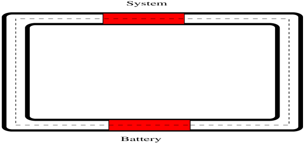
Figure 3: A closed nanocircuit: Each electron is assumed to travel around the circuit in closed orbits.

VI.2 Spin on a non-orientable space

In this section we treat non-orientable cases.  First we take a non-orientable manifold, $\mathcal{\mathbf{B}}=\mathbf{S}^{3}/\mathbf{Z}_{2}$, where $\mathbf{Z}_{2}=\left\{(1,T),(1,I)\right\}$.  From our discussion above, it was found that inequivalent ${pin}$ structures were given by $H^{1}(R\times\mathbf{S}^{3},\mathbf{Z}_{2})$.  This latter result has been found by different methods in john .  Finally, we would like to say more about the new adopted definition for equivalence by going back to the example of the projective plane that we mentioned earlier. Here however, we take a more physically motivated approach. Let $\psi^{a},a=1,2$, be a pinor field on $\mathbf{RP}_{2}$. The structure group of the frame bundle is $\mathbf{O}(2)$. Let $\{e_{i}^{a}\}$ be a local frame on the open set $U_{i}.$ The sets $U_{i}$ cover $\mathbf{RP}_{2}$ and their intersections are contractible so local sections are always well defined. On intersections $U_{i}\smallfrown U_{j}$ we have

$$e_{i}^{a}=(L_{ij})^{a}e_{i}^{a}\text{, with }L_{ij}\in\mathbf{O}(2)\>.$$ (137)

On the pinor frame level , we have

$$\psi_{i}^{a}=(S_{ij})_{b}^{a}\psi_{j}^{a}\text{, with }S_{ij}\in\mathbf{Pin}(2)\;,$$ (138)

and $\rho(S)=L$. We require that $\psi^{\dagger}\psi$ and $\psi^{\dagger}\gamma^{a}\psi$ transform as a scalar and a vector respectively. The $\gamma^{a}$ defined here are the Pauli matrices. From this we get the following conditions on $S$,

$$S^{\dagger}S = 1\>,$$ (139)

$$S^{\dagger}\gamma^{a}S = L_{b}^{a}\gamma^{b}\>.$$ (140)

To find explicit expressions, we need to choose a covering. $\mathbf{RP}_{2}$ is topologically equivalent to a disk with the boundary antipodally identified. Next we parametrize the boundary with an angle $\theta,0\preccurlyeq\theta\prec 2\pi$ . Choose a simple cover for the strip adjacent to the boundary, we will need at least three open neighborhoods. Non-trivial transition functions will be needed only as we go along the boundary. They are of the form

$$L=I\cdot e^{2i\theta}\>,$$ (141)

where $I$ is a reflection about the first axis. Using this cover, we find that $S$ must have the form $e^{i\alpha}\gamma^{1}e^{i\theta\gamma^{3}}$ . Imposing boundary conditions on $\psi(\theta)$ , we find that

$$e^{i\alpha}=\pm i\>.$$ (142)

Hence, the two $\mathbf{Pin}(2)$ structures predicted above. The phase factor $e^{i\alpha}$ is clearly due to the reflection $I$. Moreover, it is physically irrelevant and ignoring it amounts to ignoring $I,$ i.e., the non-orientability of the space.  Therefore quantum mechanics should be studied first on the orientable cover and then projected on the configuration space.

VII CONCLUSION

In summary, we have given a definition to spin structures on non-orientable manifolds by going to the orientable double cover.  This allowed us to determine the number of inequivalent spin structures using our definition of equivalence.  We also showed that in the typical structure of a nano-circuit, the nontrivial spin configuration is probably more important than the trivial one at nanometer scale. This argument is supported indirectly by the work in ref. magnus . A convincing proof of this statement will be to solve the problems with the constraints on the motion of the particle explicitly taken into account.  This is a very difficult problem. We believe the energy argument that we presented is compelling enough to continue looking into other aspects which can result from the nontrivial spin configuration.  Smaller non-orientable structures than those made by Tanda et al. should also be possible in the near future and provide an experimental test of the idea presented here.  Finally, there is one question that we did not discuss in this work and that is related to the nature of ’phase transition’ at the critical radius of ring between the two spin structures.  This is an interesting question mathematically and physically.  We are not the first to raise this question; Jarosczewicz asked a similar question regarding the spin of $\textbf{SU}(2)$ solitons jaros .  To avoid introducing one more flavor to quantize the spin, he introduced the idea of a rotating soliton which corresponds mathematically to the nontrivial paths in $\textbf{SO}(3)$.  A similar analysis to his may shed some light on the physics of our non-trivial spin configurations in a ring.

The author is very grateful to R. Chantrell who made this work possible and thanks J. Friedman for initial discussions on this subject.

References

• (1) S. Tanda, T. Tsuneta, Y. Okajima, K. Inagaki, K. Yamaya, and N. Hatakenaka, Nature 417, 397 (2002).
• (2) A. P. Balanchandran, G. Marmo, B. S. Skagerstman, and A. Stern, Classical Topology and Qunatum States, World Scientific (1991).
• (3) D. J. Thouless, Phys. Rev. B 27, 6083 (1983).
• (4) A. Rebei and O. Heinonen, spin currents in the Rashba model, submitted to Phys. Rev. textbfB.
• (5) E. Witten, Nucl. Phys. B223, 422 (1983).
• (6) L. Alvarez-Gaume and P. Ginsparg, Ann. Phys. (NY) 161, 423 (1985).
• (7) E. Saitoh, S. Kasai, and H. Miyajima, J. Appl. Phys. 97, 10J709 (2005).
• (8) P. A. Dirac, Proc. Roy. Soc. (London) A 117, 610 (1928).
• (9) H. B. Petry, J. Math. Phys. 20, 231 (1979).
• (10) L. S. Schulman, Techniques and Applications of Path integration. New York, Wiley 1981.
• (11) L. Dabrowski, Group Actions on Spinors (Bibliopolis, 1988).
• (12) M. Berg, C. DeWitt-Moretti, S. Gwo and E. Kramer, Rev. Math. Phys. 13, 953 (2001).
• (13) M. Atiyah, R. Bott and A. Shapiro, Topology 3, Suppl. 1, 3 (1964).
• (14) M. Karoubi, Ann. Scient. Ec. Norm.1, 161 (1968).
• (15) D. Ebner, Gen. Rel. Grav. 8, 15 (1977).
• (16) T. Eguchi, P. B. Gilkey, A. J. Hanson, Phys. Rep. 66, 213 (1980).
• (17) J. Milnor,  Enseig. Math. 9, 198 (1963).
• (18) A. Chamblin, Commun.Math.Phys. 164, 65 (1994).
• (19) F. Hirzebruch, Topological Methods in Algebraic Geometry(Springer-Verlag, Berlin, 1966).
• (20) E. Spanier, Algebraic Topology (Springer, New-York, 1966).
• (21) W. Greub and H. Petry, On the Lifting of Structure Groups.  In:  Bleuler,K., Petry,H., Reetz,A. (eds) Differential Geometrical Methods in Mathematical Physics II. Proceedings, Bonn 1977, pp. 217-246. Berlin: (Springer-Verlag, Berlin, 1978).
• (22) N. Steenrod, The Topology of Fiber Bundles (Princeton, 1951).
• (23) J. Negele and H. Orland, Quantum Many-Partilce Systems, Addison-Wesley, 1988.
• (24) W. Magnus and W. Schoenmaker, J. Math. Phys. 39, 6715 (1998); Phys. Rev. B 61, 10883 (2000).
• (25) J. Frohlich and U. M. Studer, Rev. Mod. Phys. 65, 733 (1993).
• (26) F. E. Meijer, A. F. Morpurgo and T. M. Klapwijk, Phys. Rev. B 66, 033107 (2002).
• (27) J. Schwinger, Phys. Rev. 82, 664 (1951).
• (28) L. S. Schulman, Phys. Rev. 188, 1139 (1969).
• (29) J. Friedman, Class.Quantum.Grav.12, 2231 (1995).
• (30) T. Jaroszewicz, Phys. Rev. D 44, 1311 (1991).