Optimal network topologies:
Expanders, Cages, Ramanujan graphs, Entangled networks and all that.

Abstract

We report on some recent developments in the search for optimal network topologies. First we review some basic concepts on spectral graph theory, including adjacency and Laplacian matrices, and paying special attention to the topological implications of having large spectral gaps. We also introduce related concepts as “expanders”, Ramanujan, and Cage graphs. Afterwards, we discuss two different dynamical features of networks: synchronizability and flow of random walkers and so that they are optimized if the corresponding Laplacian matrix have a large spectral gap. From this, we show, by developing a numerical optimization algorithm that maximum synchronizability and fast random walk spreading are obtained for a particular type of extremely homogeneous regular networks, with long loops and poor modular structure, that we call entangled networks. These turn out to be related to Ramanujan and Cage graphs. We argue also that these graphs are very good finite-size approximations to Bethe lattices, and provide almost or almost optimal solutions to many other problems as, for instance, searchability in the presence of congestion or performance of neural networks. Finally, we study how these results are modified when studying dynamical processes controlled by a normalized (weighted and directed) dynamics; much more heterogeneous graphs are optimal in this case. Finally, a critical discussion of the limitations and possible extensions of this work is presented.

I I. Introduction

Imagine you are to design a network, be it a local computer network, an infrastructure or communication network, an artificial neural network, or whatever analogous example you can think of. Suppose also that you have some restrictions to do so. First of all, the number of nodes and the total amount of links are both fixed and, second, nodes should be connected using the available links in such a way that the resulting network topology is optimal in some sense. Of course, the meaning of the word “optimal” depends on the task to be performed by the network, or in other words, depends on the nature of the dynamical process to be built on top of it.

Along this paper we study optimization of dynamical processes in networks, as exemplified by the following three cases.

Suppose we are constructing an artificial neural network, so at each node we locate a neuron (i.e. an oscillator) having some unspecified dynamical properties. In order to enhance the neural net performance we want the oscillators to be easily synchronizable synchro , i.e. to be able to reach as easily as possible a state in which them all, or at least a large fraction of them, fire (oscillate) at unison Torres ; BJK ; GG , and that state to be as robust as possible.

As a second example, imagine having a communication or technological network and wanting, for the sake of efficiency, any node to be “nearby” any other one. The simplest strategy to do so, is by constructing a star-like topology with a central node (or “hub” in the network jargon) directly connected to all the rest. In this way, any node is reachable from any other within two steps at most. However, in cases of intense traffic flow, this might not be very efficient, especially if the central hub gets overburdened or congestioned. Also, the star-like topology is very fragile to sabotage to the central node. So one could wonder what is the optimal topology avoiding the use of a privileged central hub Catalans ; Congestion ; Maritan .

For a third example, let us consider information packets traveling in a network in such a way that they disperse jumping randomly between contiguous nodes and let us require an optimum flow of information. For that, we define an ensemble of random walkers diffusing on the net, and impose the averaged first-passage time to be minimized. Which is the optimal structure? Analogously, other random-walk properties as the mixing rate Lovasz , the mean transit time or the mean return time dani could be minimized.

In all these situations the problem to be solved is very similar: finding an optimal topology under some constraints. These and similar problems have been addressed in the literature, especially in the context of Computer Science and, more recently, in the emerging field of Complex Networks Strogatz ; Laszlo ; Newman ; Porto ; AleRomu ; Boccaletti .

In this paper, we illustrate that the answer to these problems may have a large degree of universality in the sense that, even if the optimal topologies in each case are not “exactly” identical, they may share some common features that we review here. To do so, we translate these problems into the one of optimizing some invariant property of a matrix encoding the network topology. In particular, we can use adjacency, Laplacian, and normalized-Laplacian matrices depending on the particular problem under scrutiny. Spectral analysis techniques are employed to explore in a systematic way network topologies and to look for optimal solutions in each specific problem. In this context, we introduce and characterize what we call entangled networks: a family of nets with very homogeneous properties and a extremely intertwined or entangled structure which are optimal or almost optimal from different points of view.

Along this work, we focus mainly on un-weighted, un-directed, networks, not embedded in a geography or physical coordinates, and characterized by identical nodes. Changing any of these restrictions may alter the nature of the emerging optimal topologies as will be briefly discussed at the end of the paper.

The paper is structured as follows. In section II we introduce topological matrices and other basic elements of spectral graph theory, as for instance the “spectral gap”. In section III we discuss the topological implications of having a large spectral gap and illustrate the connections of this with topological optimization problems: graphs with large spectral gaps are optimal (or almost optimal) for some dynamical processes defined on networks. In section IV we present an explicit construction of optimal solutions, called by graph theorists “Ramanujan” graphs; such explicit constructions cannot be achieved for any number of nodes and links. Owing to this, in section V we discuss how to construct optimal graphs in general (for any given number of nodes and edges) by employing a recently introduced computational optimization method, enabling us to construct the so called “entangled networks”. We compare entangled networks with Ramanujan graphs in the cases when these last can be explicitly constructed, as well as with “cage graphs”, another useful concept in graph theory. In section VI we enumerate some network design problems where our results are relevant. In section VII we briefly elaborate on the connection of Ramanujan and entangled networks in the limit of large sizes with the Bethe lattice. In section VIII we discuss how the previous results are affected by analyzing dynamical processes controlled by the normalized Laplacian rather than by the Laplacian. Finally, in section IX a critical discussion of our main results, conclusions, and future perspectives is presented.

II II. Elements of spectral graph theory: spectral gaps

For the sake of self-consistency and to fix notation we start by revising some basic concepts in graph theory.

Given a network (or graph), it is possible to define the corresponding adjacency matrix, $A$, whose elements $a_{ij}$ are equal to $1$ if a link between nodes $i$ and $j$ exists and $0$ otherwise. A related matrix is the Laplacian, $L$, which takes values $-1$ for pairs of connected vertices and $k_{i}$ (the degree of the corresponding node $i$) in diagonal sites. Obviously, $L=K-A$, where $K$ is the diagonal connectivity (or degree) matrix. If the graph is undirected both $A$ and $L$ are symmetric matrices. It is easy to see that $\lambda_{1}=0$ is a trivial eigenvalue of $L$ with eigenvector $(1,1,\ldots)$ and that the eigenvalues $\lambda_{i}$ satisfy

$$0=\lambda_{1}\leq\lambda_{2}\leq\ldots\leq\lambda_{N}\leq 2k_{\text{max}},$$

where $k_{\text{max}}$ is the largest degree in the graph. The proofs of these and other elementary spectral graph properties can be found, for instance, in Chung ; Bollobas . Finally, a normalized Laplacian matrix, $L^{\prime}=K^{-1}L$, can be defined; each row is equal to the analogous row in $L$ divided by the degree of the corresponding node. This is useful to describe dynamical processes in which the total effect of neighbors is equally normalized for all sites, while in the absence of such a normalization factor sites with higher connectivity are more strongly coupled to the others than loosely connected ones. In this case we have $0\leq\lambda^{\prime}_{i}\leq 2$ for $i=1\ldots N$, where the $\lambda^{\prime}_{i}$ denote the eigenvalues of $L^{\prime}$. Clearly, for regular graphs, that is, graphs where all nodes have the same degree $k$, the two matrices $L$ and $L^{\prime}$ differ by a multiple of the identity matrix and the eigenvalues are related by $\lambda_{i}=k\lambda^{\prime}_{i}$.

Following the literature, here we consider mainly (but not only) the Laplacian spectrum, but depending on the dynamical process under consideration this choice will be changed.

In order to give a first taste on the topological significance of spectral properties, let us consider a network perfectly separated into a number of independent subsets or communities having only intra-subset links but not inter-subset connections. Obviously, its Laplacian matrix (either the non normalized or the normalized one) is block-diagonal. Each sub-graph has its own associated sub-matrix, and therefore $0$ is an eigenvalue of any of them. In this way, the degeneration of the lowest (trivial) eigenvalue of $L$ (or of $L^{\prime}$) coincides with the number of disconnected subgraphs within a given network. For each of the separated components, the corresponding eigenvector has constant components within each subgraph.

On the other hand, if the subgraphs are not perfectly separated, but a small number of inter-subset links exists, then the degeneracy will be broken, and eigenvalues and eigenvectors will be slightly perturbed. In particular relatively small eigenvalues will appear, and their corresponding eigenvectors will take “almost constant” values within each subgraph. For instance, if the number of subsets is $2$, spectral methods have been profusely used for graph bipartitioning or graph bisecting GN as follows. One looks for the smallest non-trivial eigenvalue; its corresponding eigenvector should have almost constant components within each of the two subgroups, providing us with a bipartitioning criterion. Therefore a graph with a “small” first non-trivial Laplacian eigenvalue, $\lambda_{2}$, customarily called spectral gap (or also algebraic connectivity) has a relatively clean bisection. In other words, the smaller the spectral gap the smaller the relative number of edges required to be cut-away to generate a bipartition. Conversely a large “spectral gap” characterizes non-structured networks, with poor modular structure, in which a clearcut separation into subgraphs is not inherent. This is a crucial topological implication of spectral gaps.

A closely related concept is the expansion property. To introduce it, let us consider a generic graph, $X$, and define the Cheeger or isoperimetric constant as follows. First, one considers all the possible subdivisions of the graph in two disjoint subsets of vertices: $A$ and its corresponding complement $B$. The Cheeger constant, $h(X)$, is defined as the minimum value over all possible partitions of the number of edges connecting $A$ with $B$ divided by the number of sites in the smallest of the two subsets. The Cheeger constant is larger than $0$ if and only if the graph is connected, and is “large” if any possible subdivision has many links between the two corresponding subsets. Hence, for graphs with poor community structure, the Cheeger constant is large.

In the graph-theory literature the concept of expander is introduced within this context Sarnak ; Valette : a family of expanders is a family of regular graphs with degree $k$ and $N$ nodes, such that for $N\rightarrow\infty$ the Cheeger constant $h$ is always larger than a given positive number $\epsilon$. Note that the word “expansion”, refers to the fact that the topology of the network-connections is such that any set of vertices connects in a robust way (“expands through”) all nodes, even if the graph is sparse. Obviously, for this to happen, $k$ should be larger or equal than $3$, as for $k=2$ all graphs are linear chains and can be, therefore, cut in two subgraphs by removing just one edge (arbitrarily small Cheeger constant for large system sizes).

The Cheeger constant and the expansion property can be formally related to the spectral gap by the following inequalities AB :

$${\lambda_{2}\over 2}\leq h(X)\leq\sqrt{2k\lambda_{2}}.$$ (1)

Therefore, a family of regular graphs is an expanding family if and only if it has a lower bound for the spectral gap, and the larger the bound the better the expansion. Among the applications of expander graphs are the design of efficient communication networks, construction of error-correcting codes with very efficient encoding and decoding algorithms, de-randomization of random algorithms, and analysis of algorithms in computational group theory Sarnak .

As a consequence of this, expansion properties are enhanced upon increasing the spectral gap, but spectral gaps cannot be as large as wanted, especially for large graph sizes. In the case of $k$-regular graphs (the ones for which expanders have been defined) there is an asymptotic upper bound for it derived by Alon and Boppana AB , given by the spectral gap of the infinite regular tree of degree $k$ (called Bethe tree or Bethe lattice):

$$\lim_{N\rightarrow\infty}\lambda_{2}\leq k-2\sqrt{k-1}.$$ (2)

Whenever a graph has $\lambda_{2}\geq k-2\sqrt{k-1}$ (i.e. when the spectral gap is larger than its asymptotic upper bound), it is called a Ramanujan graph. Therefore, Ramanujan graphs are very good expanders. In one of the following sections we will tackle the problem of explicitly constructing Ramanujan graphs by following the recently developed mathematical literature on this subject.

So far we have related the spectral graph to the “compactness” of a given graph; a large gap characterizes networks with poor modular structure, in which it is difficult to isolate sub-sets of sites poorly connected with the rest of the graph or, in other words, large gaps characterize expanders. In the following section we shift our attention from topology to dynamics and discuss some other interesting problems which turn out to be directly related to large spectral gaps.

III III. Large spectral gaps and dynamical processes

In this section we review two different dynamical processes defined on the top of networks and discuss how some of their properties depend on the underlying graph topology Entangled .

III.1 Synchronization of dynamical processes

An aspect of complex networks that has generated a burst of activity in the last few years, because of both its conceptual relevance and its practical implications, is the study of synchronizability of dynamical processes occurring at the nodes of a given network. How does synchronizability depend upon network topology? Which type of topology optimizes the stability of a globally synchronized statesynchro ?

A first partial answer to this question was given in a seminal work by Barahona and Pecora Pecora who established the following criterion to determine the stability of fully synchronized states on networks. Consider a general dynamical process

$$\dot{x}_{i}=F(x_{i})+\sigma\sum_{j\in n.n.i}[H(x_{j})-H(x_{i})]=F(x_{i})-\sigma\sum_{j}L_{ij}H(x_{j}),$$ (3)

where $x_{i}$ with $i\in{1,2,...,N}$ are dynamical variables, $F$ and $H$ are an evolution and a coupling function respectively, and $\sigma$ is a constant. A standard linear stability analysis can be performed by i) expanding around a fully synchronized state $x_{1}=x_{2}=\ldots=x_{N}=x^{s}$ with $x^{s}$ solution of $\dot{x^{s}}=F(x^{s})$, ii) diagonalizing $L$ to find its $N$ eigenvalues, and iii) writing equations for the normal modes $y_{i}$ of perturbations

$$\dot{y}_{i}=\left[F^{\prime}(x^{s})-\sigma\lambda_{i}H^{\prime}(x^{s})\right]y_{i},$$ (4)

all of them with the same form but different effective couplings $\alpha=\sigma\lambda_{i}$. Barahona and Pecora noticed that the maximum Lyapunov exponent for Eq. (4) is, in general, negative only within a bounded interval $[\alpha_{A},\alpha_{B}]$, and that it is a decreasing (increasing) function below (above) (see fig. 1 in Pecora , and see also the related work by Wang and Chen Wang in which the case $[\alpha_{A},\infty]$ is studied). Requiring all effective couplings to lie within such an interval, $\alpha_{A}<\sigma\lambda_{2}\leq\ldots\leq\sigma\lambda_{N}<\alpha_{B}$, one concludes that a synchronized state is linearly stable if and only if $\frac{\lambda_{N}}{\lambda_{2}}<\frac{\alpha_{B}}{\alpha_{A}}$ for the corresponding network. It is remarkable that the left hand side depends only on the network topology while the right hand side depends exclusively on the dynamics (through $F$ and $G$, and $x^{s}$).

As a conclusion, the interval in which the synchronized state is stable is larger for smaller eigenratios $\lambda_{N}/\lambda_{2}$, and therefore one concludes that a network has a more robust synchronized state if the ratio $Q=\lambda_{N}/\lambda_{2}$ is as small as possible Wang . Also, as the range of variability of $\lambda_{N}$ is limited (it is related to the maximum connectivity Mohar ) minimizing $Q$ gives very similar results to maximizing the denominator $\lambda_{2}$ in most cases. Indeed, as argued in Wang in cases where the maximum Lyapunov exponent is negative in an un-bounded from above interval, the best synchronizability is obtained by maximizing the spectral gap.

It is straightforward to verify that for normalized dynamics, i.e., problems where a quotient $k_{i}$ appears in the coupling function in Eq.(3), the Laplacian eigenvalues have to be replaced by the normalized-Laplacian ones, so the gap refers to $\lambda^{\prime}_{2}$ and $Q$ becomes $Q_{norm}=\lambda^{\prime}_{N}/\lambda^{\prime}_{2}$.

Summing up, large spectral gaps favor stability of synchronized states (synchronizability).

III.2 Random walk properties

One of the first and most studied models on graphs are random walks: these are important both as a simple models of dispersion phenomena and as a tool for exploring graph properties.

Indeed random walk properties are strictly related to the underlying network structure and, in particular, to the eigenvalue spectrum of the previously introduced matrices. At each step the transition probability from vertex $i$ to vertex $j$ is trivially given by $P_{ij}={A_{ij}\over k_{i}}$. This defines a transition matrix $P$ for random walk dynamics, that can be written as $P=K^{-1}A=K^{-1}(K-L)=I-L^{\prime}$ (where $I$ the identity matrix); therefore the eigenvectors of $P$ and $L^{\prime}$ coincide and the eigenvalues are linearly related.

In particular, the stationary probability distribution of the random walk on a graph is given by the eigenvector corresponding to the largest eigenvalue (1) of $P$, corresponding to $\lambda^{\prime}=0$. Then it is easy to see that the convergence rate of a given initial probability distribution towards its stationary distribution (also called “mixing rate”) is controlled by the second largest eigenvalue of $P$, and therefore by the spectral gap of the normalized Laplacian matrix: the larger $\lambda^{\prime}_{2}$ the faster the decay Nielsen ; Lovasz .

Another relevant property is the first passage time, $\tau_{i,j}$ between two sites $i$ and $j$, defined as the average time it takes for a random walker to arrive for the first time to $j$ starting from $i$. It can be expressed in terms of the eigenvectors ($u_{k}$) and eigenvalues of the normalized Laplacian matrix as

$$\tau_{i,j}=2M\sum_{l=2...N}{\left(\frac{u_{l,i}}{\sqrt{k_{i}}}-\frac{u_{l,j}}{\sqrt{k_{j}}}\right)^{2}\frac{1}{\lambda^{\prime}_{l}}},$$

where $M$ is the number of link of the network (see Lovasz ). For $k-$regular graphs the expression of its graph average, $\tau$, can be simplified in the following way:

$$\tau=2k\frac{N}{N-1}\sum_{l=2...N}\frac{1}{\lambda}_{l}$$ (5)

A large $\lambda_{2}$ (which imply that also the following eigenvalues cannot be small) gives an important contribution for keeping $\tau$ small. Therefore large spectral gaps are associated with short first-passage times.

Finally, random walks move around quickly on graphs with large spectral gap in the sense that they are very unlikely to stay long within a given subset of vertices, $A$, unless its complementary subgraph is very small Nielsen ; Lovasz . This idea has been exploited by Pons and Latapy PL to detect communities structures in networks by associating them to regions where random walks remain trapped for some time. In conclusion: random walks escape quickly from any subset $A$ if the spectral gap is large.

Summing up: random walks move and disseminate fluently in large spectral gap graphs. Related results, more details, and proofs of these theorems can be found, for example in Nielsen ; Lovasz .

IV IV. Explicit construction of Ramanujan Graphs

The summary of the preceeding section is that if we are aimed at designing network topologies with good synchronizability or random-walk flow properties, we need criteria to construct graphs with large spectral gaps. On the other hand, as explained before, Ramanujan graphs are optimal expanders, in the sense that a given family of them, with growing $N$, will converge asymptotically from above to the maximum possible value of the spectral gap. Even if this does not imply that for finite arbitrary values of $N$ they are optimal, i.e. that they have the largest possible spectral gap, they provide a very useful approach for the optimization of the spectral gap problem. Therefore, a good way to design optimal networks so is to explicitly construct Ramanujan graphs by following the mathematical literature on this respect Valette ; LPS ; Margulis ; Chiu .

In this section we present a recipe for constructing explicitly families of Ramanujan graphs while, in the following one, we will construct large-spectral gap networks by employing a computational optimization procedure. Readers not interested in the mathematical constructions can safely skip this section.

IV.1 The recipe

In recent years some explicit methods for the construction of Ramanujan graphs have appear in the mathematical literature LPS ; Margulis . We describe here only one of them. While the proof that these graphs, constructed by Lubotzky, Phillips and Sarnak LPS (and independently by Margulis Margulis ) are Ramanujan graphs is a highly non-trivial one, their construction, following the recipe we describe in what follows, is relatively simple and can be implemented without too much effort.

Let us consider a given group $G$ and let $S\in G$ be a subset of group elements not including the identity. The Cayley graph associated with $G$ and $S$ is defined as the directed graph having one vertex for each group element and directed edges connecting them whenever one goes from one group element (vertex) to the other by applying a group transformation in $S$. The absence of the identity in $S$ guarantees that self-loops are absent. The Cayley graph depends on the choice of the generating set $S$ and it is connected if and only if $S$ generates $G$. Indeed, this will be the only case we consider here. Note that if for each element $s\in S$ its inverse $s^{-1}$ also belongs to $S$, then the associated Cayley graph becomes undirected, which is the case in all what follows.

In the construction we discuss here, the group $G$ is given by either by $PGL(2,Z/qZ)$ or by $PSL(2,Z/qZ)$. Consider the group of $2\times 2$ matrices with elements in $Z/qZ$ (i.e. integer numbers modulo $q$, where $q$ is an odd prime number); the elements of $PGL(2,Z/qZ)$ ($PSL(2,Z/qZ)$) are the equivalence classes of matrices with non-vanishing determinant (determinant equal to one) with respect to multiplications by multiples of the identity matrix (i.e. to matrices differing in multiples of the identity are considered to be equal).

To specify the subset $S$ of Cayley graph generators, the integral quaternions $H(Z)=\{\alpha=a_{0}+a_{1}i+a_{2}j+a_{3}k:a_{i}\in Z\}$ must be introduced. Quaternions can be casted in a matrix-like form as Valette :

$$\left(\begin{array}[]{cc}a_{0}+a_{1}x+a_{3}y&-a_{1}y+a_{2}+a_{3}x\\ -a_{1}y-a_{2}+a_{3}x&a_{0}-a_{1}x-a_{3}y\end{array}\right)$$ (6)

where $x,y$ are odd prime integers, satisfying $(x^{2}+y^{2}+1)\mod q=0$. Writing quaternions in this way, it turns out that their algebra coincides with the standard algebra of matrices and the quaternion norm $|\alpha|^{2}=a_{0}^{2}+a_{1}^{2}+a_{2}^{2}+a_{3}^{2}$ is equal to the corresponding matrix determinant. Now another odd prime number $p$ has to be chosen. It can be shown that there are $8(p+1)$ elements in $H(Z)$ satisfying $|\alpha|^{2}=p$. If $p\mod 4=1$ then by taking $a_{0}$ odd and positive the number of solutions is reduced to $p+1$, while if $p\mod 4=3$ then the number of solutions is reduced to $p+1$ by taking $a_{0}$ even and requiring the first non-zero component to be positive.

If $p$ is a perfect square modulo $q$ such solutions can be mapped to a set $S$ of $p+1$ matrices belonging $PSL(2,Z/qZ)$ (to guarantee that all such matrices are distinct, one can take $q>2\sqrt{p}$). A Ramanujan graph is then built as the Cayley graph with $G=PSL(2,Z/qZ)$ using the set $S$ of generators we just constructed; the number of nodes is given by $N=q(q^{2}-1)/2$ (the number of elements of $PSL(2,Z/qZ)$) and the degree of each node is $k=p+1$ (the elements of $S$). If, otherwise, $p$ is not a perfect square modulo $q$ we map the solutions to a set $S$ of $PGL(2,Z/qZ)$ matrices and a Ramanujan graph is build as the Cayley graph with $G=PGL(2,Z/qZ)$ and the set $S$ just constructed. In this case $N=q(q^{2}-1)$ and $k=p+1$.

Putting all this together, Ramanujan graphs can be built by the following procedure Code ; Valette :

• choose values of the odd prime numbers $q$ and $p$, with $q>2\sqrt{p}$;

• associate the matrices of $PGL(2,Z/qZ)$ or $PSL(2,Z/qZ)$ (depending on the relative values of $p$ and $q$) with graph nodes;

• find the solutions of $a_{0}^{2}+a_{1}^{2}+a_{2}^{2}+a_{3}^{2}=p$, a solution of $(x^{2}+y^{2}+1)\mod q=0$ and construct the matrices according to (6);

• find the neighbors of each node by multiplying the corresponding matrix by the just constructed $p+1$ matrices, and represent them by edges.

In this way we construct regular graphs with a large spectral gap, with some restrictions on the number of nodes $N$ and the degree $k$: the degree can only be an odd prime number plus one, while the number of nodes grows as the third power of $q$.

IV.2 Topological properties of the resulting graphs

First of all, every Cayley graph is by construction a regular graph, and so are the Ramanujan graphs built following the above procedure. Moreover, Lubotzky, Phillips and Sarnak LPS proved that these graphs have a large girth (the girth, $g$, of a graph is the length of the shortest loop or cycle, if any), providing a lower bound for the $g$ which grows logarithmically with $q$ (its exact form is different in the $PSL$ and $PGL$ cases). To gain some more intuition about the properties of this family of graph, we plot in the left of figure (1) the smallest one, corresponding to $k=4$ ($p=3$) and $120$ nodes ($q=5$).

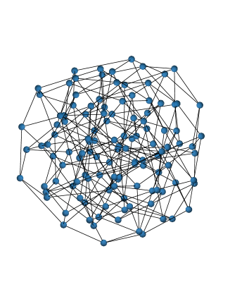
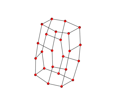
Figure 1: Ramanujan graphs with (left) degree $k=4$ ($p=3$) and $120$ nodes ($q=5$), and (right) $k=3$ ($p=2$) and $24$ nodes ($q=3$).

Some remarks on its topological properties are in order. The average distance $3.714$ is relatively small (i.e. one reaches any of the $120$ nodes starting from any arbitrary origin in less than four steps, on average). The betweenness centrality betweenness $161.5$ is also relatively small, and takes the same value for all nodes. The clustering coefficient vanishes, reflecting the absence or short loops (triangles), and the minimum loop size is large, equal to $6$, and identical for all the nodes. In a nutshell: the network homogeneity is remarkable; all nodes look alike, forming rather intricate, decentralized structure, with delta-peak distributed topological properties.

IV.3 Extension to $k=3$

P. Chiu, extended the previous method to consider also graphs with degree $3$ (i.e. $p=2$; note that the previous construction was restricted to odd prime values of $p$). To do this, one just needs to consider the following $3$ generators Chiu :

$$\left(\begin{array}[]{cc}1&0\\ 0&-1\end{array}\right),\left(\begin{array}[]{cc}2+\sqrt{-2}&\sqrt{-26}\\ \sqrt{-26}&2-\sqrt{-2}\end{array}\right),\left(\begin{array}[]{cc}2-\sqrt{-2}&-\sqrt{-26}\\ -\sqrt{-26}&2+\sqrt{-2}\end{array}\right),$$ (7)

acting on the elements of $PGL(2,Z/qZ)$ or $PGL(2,Z/qZ)$ as before.

In the right part of figure (1) we show the smallest Ramanujan graph with degree $k=3$ ($p=2$) and $24$ nodes ($q=3$). This is slightly less homogeneous than the one with $k=4$, but it is as homogeneous as possible given the previous values of $N$ and $k$. The average distance is also small in this case, $3.13$, the betweenness is $24.50$ for all nodes, the clustering vanishes, and the size of the minimum loop is $4$. While for edges, the edge betweenness betweenness is $27.31$ for $12$ edges while it is $22.34$, for the remaining $24$ edges; indicating that the net is not fully homogeneous in this case, but not far from homogeneous either.

Summing up, the main topological features of these Ramanujan graphs is that they are very homogeneous: properties as the average distance, betweenness, minimum loop size, etc are very narrowly distributed (they are delta peeks in many cases). Also, compared to generic random regular graphs, their averaged distance is smaller and the average minimum loop size is larger. A main limitation of Ramanujan graphs constructed in this way is that, for a fixed connectivity, the possible network sizes are restricted to specific, fast growing values.

V V. Construction of networks by computational optimization

An alternative route to build up optimal networks with an arbitrary number of nodes and an as-large-as-possible spectral gap or (almost equivalently) an as-small-as-possible synchronizability ratio $Q=\lambda_{N}/\lambda_{2}$ is by employing a computational optimization process. Note, that enumerating all possible graphs with fixed $N$ and $\langle k\rangle$, and looking explicitly for the minimum value of $Q$ or largest gap, is a non-polynomial problem and, hence, approximate optimization approaches are mandatory Entangled . In this section, we focus on optimizing the Laplacian spectral gap while in section VIII we will tackle the normalized Laplacian case and discuss the differences between the two of them.

V.1 The algorithm

The idea is to implement a modified simulated annealing algorithm SA which, starting from a random network with the desired number of nodes $N$ and average connectivity-degree $\langle k\rangle$, and by performing successive rewirings, leads progressively to networks with larger and larger spectral gaps or smaller and smaller eigenratios $Q$. As the spectral gap will be very large in the emerging networks, they will be typically Ramanujan graphs (whenever they are regular).

The computational algorithm is as follows Entangled . At each step a number of rewiring trials is randomly extracted from an exponential distribution. Each of them consists in removing a randomly selected link, and introducing a new one joining two random nodes (self-loops are not allowed). Attempted rewirings are (i) rejected if the updated network is disconnected, and otherwise (ii) accepted if $\delta Q=Q_{final}-Q_{initial}<0$, or (iii) accepted with probability Penna $p=\min\left(1,[1-(1-q)\delta Q/T]^{1/(1-q)}\right)$ (where $T$ is a temperature-like parameter) if $\delta Q\geq 0$. Note that, in the limit $q\to 1$ we recover the usual Metropolis algorithm. Instead we choose $q=-3$ which we have verified to give the fastest convergence, although the output does not essentially depend on this choice Penna . The first $N$ rewirings are performed at $T=\infty$. They are used to calculate a new $T$ such that the largest $\delta Q$ among the first $N$ ones would be accepted with some large probability: $T=(1-q)\cdot(\delta Q)_{max}$. Then $T$ is kept fixed for $100N$ rewiring trials or $10N$ accepted ones, whichever occurs first. Afterwards, $T$ is decreased by $10\%$ and the process iterated until there is no change during $5$ successive temperature steps, assuming that a (relative) minimum of $Q$ has been found. It is noteworthy that most of these details can be changed without affecting significatively the final results, while two algorithm drawbacks are that the calculation of eigenvalues is slow and that the dynamic can get trapped into “metastable states” (corresponding to local but not global extreme values) as we illustrate in Entangled .

Running the algorithm for different initial networks, we find that whenever $N$ is small enough (say $N\lesssim 30$), the output-topology is unique in most of the runs, while some dispersion in the outputs is generated for larger $N$ ($N=2000$ is the larger size we have optimized). This is an evidence that the $Q$ absolute minimum is not always found for large graphs, and that the evolving network can remain trapped in metastable states. In any event, the final values of $Q$ are very similar from run to run, starting with different initial conditions, as shown in fig. 2, which makes us confident that a reasonably good and robust approximation to the optimal topology is typically obtained, though, strictly speaking, we cannot guarantee that the optimal solution has been actually found, especially for large values of $N$.

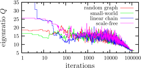
Figure 2: Eigenvalue ratio, $Q$ as a function of the number of algorithmic iterations, starting from different initial conditions (random network, small-world, linear chain, and scale free network) with $N=50$, and $\langle k\rangle=4$. The algorithm leads to topologies as the one depicted in figure 4.

V.2 Topological properties of the emerging network

In figures (3) and (4) we illustrate the appearance of the networks emerging out of the optimization procedure, that we call entangled networks, for different values of $N$ and $\langle k\rangle$.

                 

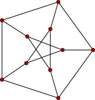
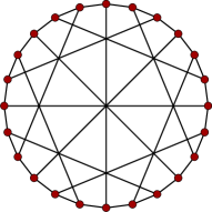
Figure 3: Optimal, entangled, networks obtained as output of the optimization procedure for $k=3$ with $N=10$ and $N=24$. The left one is a Petersen cage graph (k=3, girth=5). The one to the right is a McGee cage graph (k=3, girth=7).

Remarkably, for some small values of $N$ and $k$ (see figure (3)), it is possible to identify the resulting optimized networks with well-known ones in graph theory: cage graphs Cages ; Bollobas .

A $(k,g)$-cage graph is a $k$-regular graph with girth $g$ having the minimum possible number of nodes. Cage graphs have a vast number of applications in computer science and theoretical graph analysis Cages ; Bollobas . For $k=3$ and $N=10,14$, and $24$, respectively, the optimal nets found by the algorithm are cage-graphs with girth $5$, $6$, and $7$ respectively (called $Petersen$, $Heawood$ and $McGee$ graphs in the mathematical literature; see fig.(3) and also the nice picture gallery and mathematical details in Cages ). We also recover other cage graphs for small values of $N$ for $k=4$ and $k=5$.

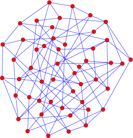
Figure 4: Optimal, entangled, network obtained as output of the optimization procedure for $k=4$ with $N=50$.

For some other small values of $N$, cage graphs do not exist. For example, for $k=3$ and girths, $3,4,5,6$, and $7$ the Cage graphs have the sizes: $N=4,6,10,14$, and $24$ respectively Cages . Therefore, for sizes as $N=12$ or $N=16$ there is no cage with $k=3$. In these cases, our optimization procedure leads to graphs similar to cages (see figure 5) in which the shortest loops are as large as possible, and all of them have very similar lengths. In this sense, our family of optimal graphs provides us with topologies “interpolating” between well known cage graphs.

                 

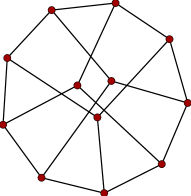
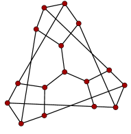
Figure 5: Optimal, entangled, networks obtained as output of the optimization procedure for $k=3$ with $N=12$ and $N=16$. They do not correspond to cage-graphs.

In the emerging entangled networks short loops are severely suppressed as said before. This can be quantified by either the girth or more accurately by the average length, $\langle\ell\rangle$, of the shortest loop from each node. In particular, the clustering coefficient (measuring the number of triangular loops in the net) vanishes, as loops have typically more than three edges.

To have a more precise characterization of the emerging topologies, especially for larger graphs (see figure (4)), we monitored different topological properties during the optimization process, as shown in figure (6).

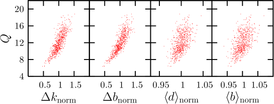
Figure 6: Relation between the ratio $Q$ and (i) node-degree standard deviation, (ii) betweenness standard deviation, (iii) average node-distance, and (iv) average betweenness. The subscript “norm” stands for normalization with respect to the respective mean-values, centering all the measured quantities around $1$. They all decrease on average as the optimization procedure goes.

The node-degree standard deviation typically decreases as $Q$ decreases meaning that the optimal topology approaches a regular one. The betweenness standard deviation also decreases with $Q$ implying that optimal networks tend to be as homogeneous as possible, and that all nodes play essentially the same role in flow properties. Also, the average node distance and average betweenness are progressively diminished on average: nodes are progressively closer to each other and the network becomes less centralized as the optimization procedure runs. It has also been numerically verified that the average first passage times of random walk is reduced during the network optimization.

The fact that the betweenness distribution is very narrow, indicates that (following an original idea by Girvan and Newman GN ) it is very difficult to divide the network into communities. Indeed, in the algorithm proposed in GN to identify communities, links with high betweenness centrality are progressively cut out; if all links have the same centrality the method becomes useless and communities are hardly distinguishable.

We have named the emerging structures entangled networks, to account for their very intricate and interwoven topology, with extremely high homogeneity in different topological properties, poor modularity or community structure, and large loops. In particular, as the spectral gap is very large and they tend to be regular, entangled nets are usually Ramanujan graphs.

We have also exploited our understanding of the entangled-topology to generate optimal networks more efficiently. In particular, given the convergence in all the explored cases to almost regular networks, we have constructed an improved version of the algorithm in which we start with random regular nets and rewire edges in such a way that the original degree distribution is preserved (indeed, most of the entangled networks depicted in this section are obtained using this improved algorithm). For this, links are selected by pairs, an origin node is selected for each one and the two end nodes are exchanged as shown in figure 7. We have observed numerically that the convergence towards optimal solutions is faster when constraining the optimization to the regular networks and that for large values of $N$ the final outputs have smaller values of $Q$ than the original ones (owing to the fact that it is less likely to fall into metastable states). The discussed topological traits remain unaffected.

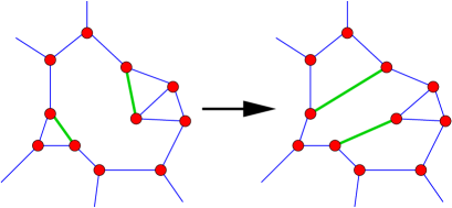
Figure 7: Rewiring attempt in the connectivity conserving version of the algorithm.

V.3 Comparing Cayley-graph Ramanujans with Entangled networks

V.3.1 Small sizes: Cage graphs

If we are to design optimal networks with a small number of vertices (say $N<100$) then entangled networks (and hence, cage-graphs, whenever they exist) are a better choice than Ramanujan nets based on Cayley-graphs, as those constructed in the previous section. First, these second do exist only for a few small values of $N$. Second, because even when such Ramanujan graphs exist entangled network outperform them, as they have a smaller value of $Q$ (larger spectral gap) which has been optimized on-purpose.

V.3.2 Large sizes

For large values of $N$ (say $N>100$) entangled networks are difficult to construct as the optimization algorithm becomes not affordably time-consuming. Instead, Cayley-graph Ramanujan networks, whenever they can be constructed, are a better choice. They are easy and fast to construct by following the recipe described in a previous section and they provide large spectral gaps, closer and closer to the optimal value (asymptotic upper bound) as $N$ increases.

VI VI. Related problems and similar topologies

In this section we illustrate how entangled networks and Ramanujan graphs play a crucial role in different contexts, and emerge as optimal (or close to optimal) solutions for a number of network optimization problems.

VI.1 Local search with congestion

This is one of the examples illustrated in the introduction, and has been recently tackled by Guimerá et al. Catalans . By defining an appropriate search cost function these authors explore which is the ideal topology to optimize searchability and facilitate communication processes. They arrive at the conclusion that, while in the absence of traffic congestion a star-like (centralized) topology is the optimal one (as briefly discussed in the introduction) when the density of information-packets traveling through the net is above a given threshold (i.e. when there is flow congestion) the optimal topology is a highly homogeneous one. In this last, all nodes have essentially the same degree, the same betweenness, and short loops are absent (see figure 1 in Catalans ). These networks resemble enormously the entangled and Ramanujan nets described above.

For a similar comparison between centralized and de-centralized transport in networks, see Congestion . Also here, decentralized, highly homogeneous, structures emerge as optimal ones under certain circumstances.

VI.2 Network structures from selection principles

In a recent letter, Colizza et al. Maritan have addressed the search of optimal topologies by using different selection principles. In particular they minimize a global cost function defined as

$$H_{\alpha}=\sum_{i<j}d_{ij}(\alpha)$$ (8)

with

$$d_{ij}(\alpha)=\min_{P}\sum_{p\in P:i\rightarrow j}k_{p}^{\alpha}.$$ (9)

This is, the cost function is the sum over pairs of sites of their relative $\alpha$-dependent distance. The distance between two nodes is the minimum of the sum of $k_{p}^{\alpha}$ ($k_{p}$ is the degree of node $p$) over all possible paths connecting the two nodes. In this way, for $\alpha=0$ the standard distance is recovered. On the other hand, for large values of $\alpha$, highly connected vertices (hubs) are strongly penalized. In this way, and rephrasing the authors of Maritan , the generalized definition of the distance “captures the conflict between two different trends: the avoidance of long paths and the desire to skip heavy traffic”. For small values of $\alpha$ (standard distance) the best topology include central hubs (centralized communication), while for $\alpha>1$ the dominant tendency is towards degree minimization, leading to open tree-like structures. For intermediate cases, i. e. $\alpha=0.5$ topologies extremely similar to entangled networks, with long loops and very high homogeneity, have been reported to emerge (see figure 3c in Maritan ).

VI.3 Performance of neural networks

Recently Kim concluded that neural networks with a clustering coefficient as small as possible exhibit much better performance than others BJK . Entangled nets have a very low clustering coefficient as only large loops exist and, therefore, they are natural candidates to constitute an excellent topology to achieve good performance and high capacity in artificial neural networks.

VI.4 Robustness and resilience

The problem of constructing networks whose robustness against random and/or intentional removal is as high as possible has attracted a lot of attention. In particular, in a recent paper 2peak , it has been shown that for generalized random graphs in the limit $N\to\infty$ the most robust topology (in the sense that the corresponding percolation threshold is as large as possible) has a degree distribution with no more than $3$ distinct node connectivities; i.e. with a homogeneous degree-distribution as homogeneous as possible.

To study the possible connection with our extremely homogeneous entangled networks, let us recall that the topology we have considered to initialize the improved version of the optimization algorithm (i.e. random $k$-regular graphs) is already the optimal solution for robustness-optimization against (combined) errors and attacks in random networks 2peak . A natural question to ask is whether further $Q$-optimization has some effect on the network robustness. This and related questions have been analyzed in Entangled , where it was shown that indeed, $Q$ minimization implies a robustness improvement. This occurs owing to the generation of non-trivial correlations in entangled structures, which place them away from the range of applicability of the result in 2peak (they are not random networks). Hence, entangled networks are also extremely efficient from the robustness point of view. This conclusion also holds for reliability against link removal Myrvold .

VII VII. The connection with the Bethe lattice

In this section we will show how entangled networks are related to the infinite regular tree called Bethe lattice (or Bethe tree) in the physics literature.

Intuitively, whenever around a given node of a regular graph only large loops are present, the neighborhood of such node looks as the one in a Bethe tree, up to a distance equal to the half of the shortest loop length (see for instance the center of the graph depicted to the right of figure 5). Therefore, if the girth diverges in a family of graphs, the neighborhood of each node tends to look locally like a Bethe, up to a growing distance.

We notice that the asymptotic spectral gap of regular graphs is bounded by the one of the Bethe tree, $\lambda_{2}\leq k-2\sqrt{k-1})$ (see equation (2)) bethegap . We can express this bound in terms of the spectral properties of the adjacency matrix (since the graphs are regular, the results can be easily translated to $L$ and $L^{\prime}$).

The moments $m_{n}$ of the adjacency matrix eigenvalues $\mu_{i}$ can be trivially expressed through the trace of the $n$-th power of $A$ LPS :

$$m_{n}=\frac{1}{N}\sum_{i}\mu_{i}^{n}=\frac{1}{N}\sum_{i}(A^{n})_{ii}.$$ (10)

It is easy to see that the diagonal elements of $A^{n}$ represent the number of paths of length $n$ starting and ending at the corresponding node. Clearly, if $n$ is smaller than the girth of the graph the paths do not contain loops and their number is equal to the number of such paths for a node of the Bethe lattice and therefore equal for all the nodes. The eigenvalue moments for the infinite Bethe lattice can be obtained in a similar way, with the only difference that the eigenvalue distribution is now a continuous spectral density density . The sum in equation (10) is now an integral and the adjacency matrix is a linear operator; however it is still possible to express the $n$-th moments as the number of length-$n$ paths from a node to itself. As a result the moments $m_{n}$ of the adjacency matrix eigenvalues of a regular graph with girth $g$ are equal to the moment of the spectral density

$$\rho(\mu)=\frac{k\sqrt{4(k-1)-\mu^{2}}}{2\pi(k^{2}-\mu^{2})}\ ,\quad\text{for }|\mu|\leq 2\sqrt{k-1}$$ (11)

of the Bethe tree bethedensity , for every $n<g$.

The previous argument can be generalized and it can be rigorously proven mckay that for an infinite sequence $G_{n}$ of $k$-regular graphs, if the number of loops of length $l$ grows slower than the number of nodes for every $l$ then, the spectral density tends to the one in equation (11). Hence, we expect a fast convergence for graphs with large girth as the ones discussed before.

To illustrate this, in figure 8 we plot the Bethe lattice integrated spectral density as a function of the eigenvalues for $k=4$ and compare it with the one calculated for a Ramanujan graph with $6840$ nodes ($q=19$) and also $k=4$ ($p=3$). The agreement is very remarkable given the finite size of the Ramanujan graph.

Figure 8: Integrated spectral density as a function of the adjacency matrix eigenvalues for the Bethe lattice (infinite size) and for a Ramanujan graph with $N=6840$, both with $k=4$.

Therefore, both from the (local) topological and the spectral point of view, a family of entangled networks (or Ramanujan graphs) with growing size and girth can be used as the best possible way to approach infinite Bethe lattices with a sequence of finite lattices. This would have applications in a vast number of problems in physics, for which exact solutions in the Bethe lattice exist, but comparisons with numerics in sufficiently large lattices are difficult to obtain. In particular, approximations of Bethe lattice obtained by truncating the number of generations (Cayley trees) include a large (extensive) amount of boundary effects (losing the original homogeneity) and are therefore not a convenient finite approximation. Good approximations should avoid strong boundary effects and preserve the Bethe lattice homogeneity, and entangled networks can play such a role.

VIII VIII. A way out of homogeneity: weighted dynamics

While most of the literature on synchronization refers to Laplacian couplings as specified by equation (3), different coupling functions can be relevant in some contexts. For example, another natural choice would be

$$\dot{x}_{i}=F(x_{i})+{\sigma\over k_{i}}\sum_{j\in n.n.i}[H(x_{j})-H(x_{i})]=F(x_{i})-{\sigma\over k_{i}}\sum_{j}L_{ij}H(x_{j}),$$ (12)

relevant in cases where the joint effect of the $k_{i}$ neighbors of node $i$ is normalized by the connectivity $k_{i}$. With this type of dynamics, the effect of neighbors has the same weight for all nodes, while in the absence of the normalization factor, $k_{i}$, sites with higher connectivity are more strongly coupled to their neighbors than loosely connected ones. This describes properly real-world situations, as for instance neural networks, where the influence of the neighboring environment on the node dynamics does not grow with the number of connections. Observe that, even if the underlying topology is unweighted and undirected, the normalization factor is such that the dynamics is directed and weighted, owing to the presence of $k_{i}$ in eq.(12).

In a recent paper Motter and coauthors have undertaken a study of synchronizability by using a generalization of the previous normalized dynamics eq.(12), by employing a normalization factor $k_{i}^{\beta}$, with $\beta\geq 0$ Zhou . These authors conclude that the most robust network synchronizability is obtained for $\beta=1$, which leads back to Eq.(12).

What is the influence of the normalization factor on the results reported on this paper?

First of all, the optimal synchronizability problem, as discussed in section III, can be straightforwardly translated for the new dynamics just by replacing Eq.(3) by Eq.(12). The optimal topology for synchronizability in “normalized” dynamical processes is that minimizing the eigenratio $Q_{norm}=\lambda^{\prime}_{N}/\lambda^{\prime}_{2}$, ($\lambda^{\prime}_{i}$ denote the normalized Laplacian eigenvalues). Hence, by employing the normalized dynamics, we have a new class of optimization problems, analogous but different to the ones studied before along this paper.

We have implemented different versions of our modified simulated annealing algorithm (in its more general, not degree-conserving, version) to optimize either $Q_{norm}$ or the normalized spectral gap $\lambda^{\prime}_{2}$. After going through the optimization algorithm with normalized-Laplacian eigenvalues, as described in section V, one observes that the emerging optimally synchronizable nets have a non-homogeneous structure. For some relatively small values of $N$ and $\langle k\rangle=3$ the optimal topologies are shown in figure 9, while in figure 10 we depict an optimal net with $100$ nodes.

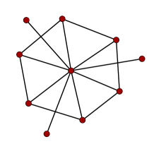
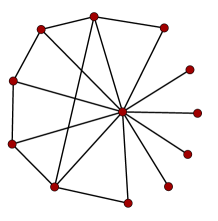
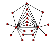
Figure 9: Optimal nets for normalized-Laplacian dynamics, with $\langle k\rangle=3$ and $N=10,12$, and $20$ respectively.

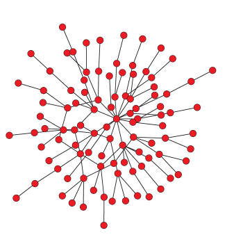
Figure 10: Optimal net for normalized-Laplacian dynamics, with $\langle k\rangle=3$ and $N=100$.

Observe the remarkable difference with previously studied networks: here homogeneity is drastically reduced. To illustrate this, in figure 11 we plot the degree distribution obtained when optimizing for $\langle k\rangle=4$ with $N=200$ and $N=1000$ respectively. The resemblance between these two distributions seems to indicate that a limit degree-distribution exists. Roughly speaking it decays faster than exponentially, but still with a much higher degree of heterogeneity than before where we had delta-peaked distributions.

The new emerging topologies exhibit a competition between the existence of central nodes and peripheral ones similarly to the networks studied in Congestion . By maximizing the spectral gap $\lambda^{\prime}_{2}$, rather than $\lambda^{\prime}_{N}/\lambda^{\prime}_{2}$ we obtain very similar results (not shown here). These new optimal topologies are very similar to those obtained by Colizza et al. Maritan in cases where the minimization of node-degree dominates (see figure 3d in Maritan ).

Let us remark that for the normalized-Laplacian, some eigenvalues bounds, analogous to those for $L$ exist; in particular Chung

$$0<\lambda^{\prime}_{2}\leq{N\over N-1}\leq\lambda^{\prime}_{N}\leq 2.$$ (13)

However, concepts analogous to “expanders” or “Ramanujan” have not been defined for general, non-regular, graphs.

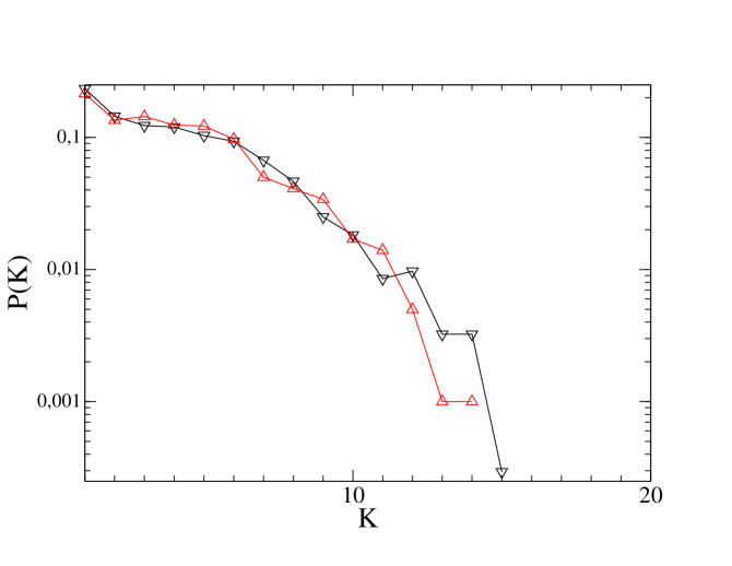
Figure 11: Semi-logarithmic plot of the degree distribution of optimal weighted networks with $\langle k\rangle=4$ and (i) $N=200$ averaged over $17$ runs (black curve with down-triangles) and (ii) $N=1000$ for a single run (red curve with up-triangles).

Finally, it is interesting to observe that our results are in apparent contradiction with the conclusion by Motter et al. Zhou that for their case $\beta=1$, corresponding to our normalized Laplacian, and large sufficiently random networks the eigenratio $Q$ does not depend on details of the network topology, but only on its mean degree Zhou . If this was indeed the case for any network topology, our optimization procedure would be pointless. Instead, applying the minimization algorithm, starting from any arbitrary finite random network, we observe a progressive $Q$ optimization, and highly non-trivial non-random optimal structures are actually generated. This apparent contradiction is likely to be due to the building up of non-trivial correlations during the optimization process, which converts our network into highly non-random structures far away from the sufficiently random requirement in Zhou .

IX IX. Discussion and Conclusions

In this paper we have reviewed recent developments in the design of optimal network topologies.

First of all we have related the problem of finding optimal topologies for many dynamical and physical problems, such as optimal synchronizability and random walk flow on networks, to the search of networks with large spectral gaps. This connection allows us to relate optimal networks to expanders and Ramanujan graphs, well-known concepts in graph-theory which, by construction, have large spectral gaps. In one of the sections we have given, following the existing mathematical literature, a recipe to explicitly construct Ramanujan graphs.

On the other hand, we have employed a simulated annealing algorithm which selects progressively networks with better synchronizability, i.e. networks with larger spectral gaps. When applied to problems with un-normalized Laplacian dynamics this algorithm leads to what we call “entangled” topologies. These are optimal expanders, and can be loosely described as being extremely homogeneous, having long loops, poor modularity, and short node-to-node distances. They are optimal or almost optimal for many different communication and flow processes defined on regular networks. In particular these topologies are relevant for the design of efficient communication networks, construction of error-correcting codes with very efficient encoding and decoding algorithms, de-randomization of random algorithms, traffic problems with congestion, and analysis of algorithms in computational group theory. Remarkably, they also provide a good finite-size approximation to Bethe lattices.

Even though these topologies play an important role in human-designed networks, especially in Computer Science and Algorithmics, they do not seem to appear frequently in Nature. Indeed, most of the topologies described in recent years for biological, ecological, social, or technological networks exhibit a very heterogeneous scale-free degree distribution Strogatz ; Laszlo ; Newman ; Porto ; AleRomu ; Boccaletti , at odd with the extremely homogeneous entangled topologies. To justify this, first of all we should emphasize that optimal entangled networks are obtained performing a global optimization procedure, which might be not very realistic. For example, by adding a new node to a given optimal network, in some cases the full entangled topology has to be altered to convey with the requirement of maximizing the spectral gap. This is certainly impractical for growing networks.

On the other hand, we should also note that there are ingredients that could be (and actually are) relevant for the determination of optimal networks in real-world problems and that have not being considered here. A non exhaustive list of examples is:

• nodes might be non equivalent,

• links could support different variable weights,

• directed networks might be mandatory in some cases,

• in some real-world networks nodes are embedded into a geography and, therefore, the distances between them should be taken into account as a sort of quenched disorder (see for instance, Gastner ; Barthelemy for application to communication infrastructures).

However, our entangled networks are still relevant for any type of un-directed un-weighted networks in which none of these effects plays an important role, and where communication properties are to be maximized. Numerous examples have being cited above and along the paper.

In the last section of the paper, we have “enlarged our horizon” by studying a different type of dynamical processes, that could be argued to be more realistic in some circumstances: instead of analyzing Laplacian coupling between the network nodes we shifted to the study of normalized-Laplacian coupling, which lead to weighted and directed dynamics. This is characterized by the presence of a “normalized dynamics” in which the relative influence of the neighbors on a given site does not depend on the site connectivity. In particular, this type of dynamics might be more adequate to describe random walks and general diffusion processes on general (not necessarily regular) networks. In this case, an optimization procedure analogous to the one described before, leads to much more heterogeneous optimal topologies, including hubs, and a much broader degree distribution. This makes the emerging optimal networks closer to real-world topologies than entangled networks, while still keeping the global-optimization perspective. Along this same line of reasoning, other alternative types of dynamics could be introduced, as for instance the “load-weighted” ones first proposed in Chavez ; Zhou as a generalization of the normalized-Laplacian dynamics. A very interesting, open question, is to define optimization processes along the lines of this paper, leading to scale free topologies.

We hope this work will encourage further research on this fascinating question of optimal network topologies, their evolution, their application to human designed networks and their connection with real-world complex networks.

- (1) T. Nishikawa, A. E. Motter, Y.-C. Lai, and F. C. Hoppensteadt, Phys. Rev. Lett. 91, 014101 (2003). H. Hong, B. J. Kim, M. Y. Choi, and H. Park Phys. Rev. E. 69, 067105 (2004). H. Hong, M. Y. Choi, and B. J. Kim, Phys. Rev. E 65, 026139 (2002); Phys. Rev. E 65, 047104 (2002).
- (2) J. J. Torres, M. A. Muñoz, J. Marro, and P. L. Garrido, Neurocomputing, 58-60, 229 (2004); and references therein.
- (3) B. J. Kim, Phys. Rev. E 69, 045101(R) (2004). See also, P. McGraw and M. Menzinger, Phys. Rev. E 72, 015101(R) (2005).
- (4) G. Grinstein and R. Linsker, Proc. Natl. Acad. Sci. USA, 102, 9948 (2005).
- (5) R. Guimera, A. Arenas, A. Diaz-Guilera, F. Vega-Redondo, A. Cabrales, Phys. Rev. Lett. 89, 248701 (2002).
- (6) D. J. Ashton, T. C. Jarrett, and N. F. Johnson, Phys. Rev. Lett. 94, 058701 (2005).
- (7) V. Colizza, J. R. Banavar, A. Maritan, and A. Rinaldo, Phys. Rev. Lett. 92, 198701 (2004).
- (8) L. Lovász, in Combinatorics, Paul Erdös is Eighty (V2), Keszthely, Hungary, pp. 1-46, (1993).
- (9) E. M. Bollt and D. ben-Avraham, New Journal of Phys. 7, 26 (2005).
- (10) S. H. Strogatz, Nature 410, 268 (2001).
- (11) A. L. Barabási, Rev. Mod. Phys. 74, 47 (2002).
- (12) M. E. J. Newman, SIAM Review 45, 167 (2003).
- (13) S. N. Dorogovtsev and J. F. F. Mendes, Evolution of Networks: From Biological Nets to the Internet and WWW, Oxford University Press, Oxford (2003).
- (14) R. Pastor Satorras and A. Vespignani, Evolution and Structure of the Internet: A Statistical Physics approach, Cambridge University Press (2004).
- (15) S. Boccaletti, V. Latora, Y. Moreno, M. Chavez, and D.-U. Hwang, Phys. Rep. 424, 175 (2006).
- (16) F. Chung, Spectral Graph Theory, Number 92 in CBMS Regional Conference Series in Mathematics. Am. Math. Soc., 1997. See also, F. Chung, L. Lu, and V. Vu, Internet Mathematics, I, 257 (2004).
- (17) B. Bollobás, Extremal Graph Theory Academic Press, New York. 1978. W. Tutte, Graph Theory As I Have Known It, Oxford U. Press, New York, (1998).
- (18) M. Girvan, M. E. J. Newman, Proc. Natl. Acad. Sci. USA 99, 7821-7826 (2002). M. E. J. Newman, M. Girvan, Phys. Rev. E 69, 026113 (2004). See also, L. Donetti and M. A. Muñoz, J. Stat. Mech.: Theor. Exp. (2004) P10012; in “Modeling Cooperative behavior in the social sciences”, AIP Conf. Proc. 779, 104 (2005); arXchic:Physics/0504059.
- (19) P. Sarnak, Notices Amer. Math. Soc. 51, 762 (2004).
- (20) G. Davidoff, P. Sarnak, and A. Valette, Elementary Number Theory, Group Theory and Ramanujan Graphs, London Math. Soc. Students Texts, 55, Cambridge (2003).
- (21) The original statement of the lower bound is due to N. Alon and R. Boppana, and appears in A. Nilli, Discrete Math., 91, 207 (1991).
- (22) L. Donetti, P. I. Hurtado and M. A. Muñoz, Phys. Rev. Lett. 95, 188701 (2005).
- (23) M. Barahona and L. M. Pecora, Phys. Rev. Lett. 89, 054101 (2002). See also, L. M. Pecora and T. L. Carroll, Phys. Rev. Lett. 64, 821 (1990); ibid, 80, 2109 (1998). L. M. Pecora, Phys. Rev. E 58 347 (1998). L. M. Pecora and T. L. Carroll, Phys. Rev. Lett. 80, 2109 (1998).
- (24) X. F. Wang and G. Chen, Int. J. Bifurcation Chaos Appl. Sci. Eng. 12, 187 (2002). X. F. Wang and G. Chen, IEEE Trans. Circuits and Systems I 49, 54 (2002).
- (25) B. Mohar, in Graph Theory, Combinatorics, and Applications, Vol 2, Ed. Y. Alavi, G. Chartrand, O. R. Oellermann, and A. J Schwenk, Wiley, New York, 1991. pp. 871.
- (26) . See also,
- (27) P. Pons and M. Latapy, Preprint. arXiv:physics/0512106.
- (28) A. Lubotzky, R. Phillips, and P. Sarnak, Combinatorica, 8, 261 (1988).
- (29) G. A. Margulis, Prob. of Info. Trans. 9, 325 (1975). See also, O. Reingold, S. Vadhan, and A. Wigderson, Ann. of Math. 155, 157 (2002).
- (30) P. Chui, Combinatorica, 12, 275 (1992).
- (31) Our computer code to generate Ramanujan graphs is available upon request to any of the authors.
- (32) The betweenness centrality is defined as the average number of shortest paths, connecting every possible couple of nodes, passing through each site. An edge-betweenness can be analogously defined for the number of shortest paths passing through each link.
- (33) S. Kirkpatrick, C. D. Gelatt, and M. P. Vecchi, Science 220 671 (1983). N. Metropolis, A. W. Rosenbluth, M. N. Rosenbluth, A. H. Teller, and E. Teller, J. Chem. Phys. 21 1087 (1953).
- (34) T. J. P. Penna, Phys. Rev. E 51, R1 (1995).
- (35) Eric W. Weisstein. ”Cage Graph.” From MathWorld–A Wolfram Web Resource. ; and references therein. See also, R. C. Read and R. J. Wilson,An Atlas of Graphs, Oxford, England: Oxford University Press, pp. 263 and 271-274, 1998.
- (36) A.X.C.N. Valente, A. Sarkar, and H.A. Stone, Phys. Rev. Lett. 92, 118702 (2004).
- (37) W. Myrvold, Proceedings of the Int. Conf. on Graph Theory, Combinatorics, Algorithms, and Applications, Vol. II, pag. 650 (1998).
- (38) See D. Cassi, Phys. Rev. B 45, 454 (1992); and references therein.
- (39) Note that as the tree is infinite, its spectrum is continuous, and therefore, it is more meaningful to refer to “spectral densities”.
- (40) H. Kesten, Trans. AMS 92, 336 (1959).
- (41) B. D. McKay, Linear Algebra and its applications 40, 203 (1981)
- (42) D. Cassi, F. Neri, L. Donetti, and M.A. Muñoz; preprint 2006.
- (43) A. E. Motter, C. Zhou, and J. Kurths, Phys. Rev E 71, 016116 (2005); AIP Conference Proceedings 776, 201 (2005); EuroPhys. Lett. 69, 334 (2005).
- (44) M. T. Gastner and M. E. J. Newman, arXiv:cond-mat/0603278.
- (45) M. Barthelemy and A. Flammini, arXiv:physics/0601203.
- (46) M. Chavez, D.-U. Hwang, A. Amann, H. G. E. Hentschel, and S. Boccaletti, Phys. Rev. Lett. 94, 218701 (2005).