Efficiency of Information Spreading in a population of diffusing agents

Abstract

We introduce a model for information spreading among a population of $N$ agents diffusing on a square $L\times L$ lattice, starting from an informed agent (Source). Information passing from informed to unaware agents occurs whenever the relative distance is $\leq 1$. Numerical simulations show that the time required for the information to reach all agents scales as $N^{-\alpha}L^{\beta}$, where $\alpha$ and $\beta$ are noninteger. A decay factor $z$ takes into account the degeneration of information as it passes from one agent to another; the final average degree of information of the population, $\mathcal{I}_{av}(z)$, is thus history-dependent. We find that the behavior of $\mathcal{I}_{av}(z)$ is non-monotonic with respect to $N$ and $L$ and displays a set of minima. Part of the results are recovered with analytical approximations.

I Introduction

The information spreading in a population constitutes an attracting problem due to the emerging complex behavior and to the great number of applications born ; llas ; moreno ; hed . The propagation of information can be seen as a sequence of interpersonal processes between the interacting agents making up the system. In general, the population can be represented by a graph where agents are nodes and links between them exist whenever they interact with each other.

Authors, who previously investigated the diffusion of information according to such a model, introduced different kinds of interpersonal interaction, but almost all of them assumed a static society moreno ; guardiola ; brajendra (a notable exception being that of Eubank et al. eubank ). In fact, networks are usually built according to a priori rules, which means that agents are fixed at their positions and can only interact with their (predetermined) set of neighbors (the flow of information between two agents is permanently open for linked pairs of agents and permanently closed for non-linked pairs).

On the other hand, real systems are far from being static: nowadays individuals are really dynamic and continuously come in contact, and lose contact, with other people. Hence, the interactions are rather instantaneous and time-dependent, and so should be considered the links of the pertaining graph. The network should be thought of as continuously evolving, adapting to the new interpersonal circumstances.

Indeed, in sociology, where information spreading throughout a population is a long-standing problem rapoport , it is widely accepted that processes of information transmission are far from deterministic. Rather, they should incorporate some stochastic elements arising, for example, from “chance encounters with informed individuals” allen .

Sociologists also underline that, irrespective of the kind of object to be transmitted, a realistic model should take into account whether the object passed from one agent to another is modified during the process borgatti . Especially information, which spreads by replication rather than transference, is continuously revised while flowing throughout the network. Degradation during transmission processes could reveal important qualitative and quantitative effects, as some recent works zhongzhu ; lopez started to point out.

This paper introduces a model that takes into account both the issues discussed above, namely, a mobile society and information changing during transmission. The model is based on a set of random walkers meant as “diffusing individuals”: a population of $N$ interacting agents embedded on a finite space is represented by $N$ random walkers diffusing on a square $L\times L$ lattice. We assume that two or more of them can interact if they are sufficiently close to each other: as a result, a given agent has no fixed position nor neighbors, but the set of agents it can interact with is updated at each instant.

The information carried by an agent is a real (i.e., not boolean) variable, whose value lies between 0 and 1. This (together with the diffusive dynamics) is the main point that differentiates our model from the susceptible-infected (SI) contact model of virus spreading in epidemiological literature anderson , where only two status, susceptible and infected, are available to an agent. The issue of information changing is dealt with by introducing a decay constant $z\leq 1$, which measures the corruption experienced by the piece of information when passing from an agent to another. We assume $z$ to be universal: the more passages the information has undergone before reaching an individual, the more altered it is with respect to its original form.

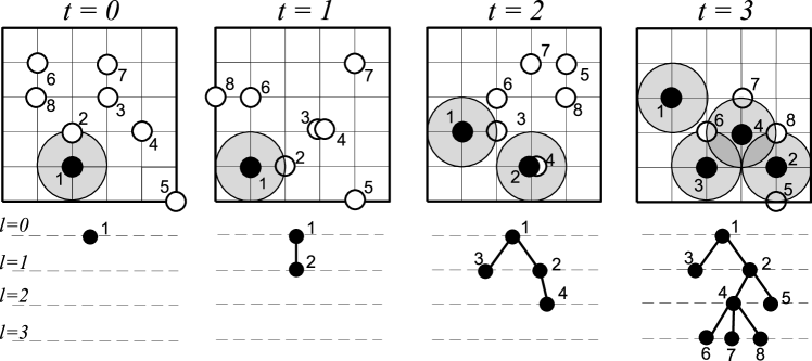
Figure 1: Evolution of 8 agents on a $5\times 5$ lattice for $t$ from 0 to 3. For each $t$ the lattice is shown above and the Information Tree is shown below. Informed agents are black circles; unaware agents are white circles. A grey circle of radius 1 is drawn around every informed agent to represent its action (an agent is in contact with another if it falls within this circle). $\mathbf{t=0}$: the only informed agent is the Information Source which carries information 1, so $n(0,0)=1$ and $n(0,l)=0$ for $l>0$. $\mathbf{t=1}$: agent 1 passes information to agent 2; now $n(1,0)=1$, $n(1,1)=1$; $\mathbf{t=2}$: agent 1 passes information to agent 3 and agent 2 passes information to agent 4; $n(2,0)=1$, $n(2,1)=2$, $n(3,1)=1$; $\mathbf{t=3}$: agent 2 passes information to agent 5; agent 4 passes information to agents 6, 7, 8. Notice that agent 6 is in contact with both 3 and 4; it chooses randomly to get information from 4 (the same for agent 8). Now all agents have been informed: for this simulation the Population-Awareness Time is $\tau=3$. The final information is $\mathcal{I}(\tau)=\sum_{l=0}^{\tau}n(l,\,\tau)z^{l}=1+2\,z+2\,z^{2}+3\,z^{3}$.

We study the time it takes for the piece of information to reach every agent (Population-Awareness Time). We show that it depends on $N$ and $L$ as a power-law, whose exponents are constant with respect to system parameters. We also investigate the final average (per agent) degree of information $\mathcal{I}_{av}(z)$. We show that $\mathcal{I}_{av}(z)$ is not a monotonic function of the density $\rho=\frac{N}{L^{2}},$ but displays minima for definite values of $N$, $L$. This interesting result implies that there does not exist a trivial direction where to tune the system parameters $N$ and $L$ in order to make information spreading more efficient.

In the following, we first describe our model (Sec. II), then we expose results obtained by means of numerical simulations (Sec. III). Next, Sec. IV contains analytical results which corroborate and highlight the former. Finally, Sec. V is devoted to our conclusions and perspectives.

II The model

$N$ random walkers (henceforth, agents) move on a square $L\times L$ lattice with periodic boundary condition. At time $t=0$ the agents are randomly distributed on the lattice. At each instant $t>0$ each agent jumps randomly to one of the four nearest-neighbor sites. There are no excluded-volume effects: there can be more agents on the same site; $\rho=N/L^{2}$ is the density of agents on the lattice.
Each agent $j$ carries a number $I_{j}$, $0\leq I_{j}\leq 1$, representing information; an agent is called “informed” if $I_{j}>0$ and “unaware” if $I_{j}=0$. At $t=0$ one agent, say agent 1, carries information 1 and is called the Information Source (or simply the Source); the other $N-1$ agents are unaware. The aim of the dynamics is to diffuse information from the Source to all agents.
Interaction between two agents $j$ and $k$ takes place when i) one of them is informed and the other unaware, and ii) the chemical distance between the two agents is $\leq 1$ (i.e., they are either on the same site or on nearest-neighbor sites: we then say that they are “in contact”). By “interaction” we mean an information passing from the informed agent, say $j$, to the unaware one $k$ with a fixed decay constant $z$ ($0\leq z\leq 1$): if $j$ carries information $I_{j}$, then $k$ becomes informed with information $I_{k}=z\,\cdot I_{i}$. Once an agent has become informed, it will never change nor lose its information (that is, informed agents never interact). If an unaware agent comes in contact with more informed agents at the same time, each carrying its own information $I_{j}$, it will acquire the information of one of them chosen at random (multiplied by $z$). The simulation stops at the time $\tau$ when all the agents have become informed: we call this the Population-Awareness Time (PAT).
We define $n(t)$ the total number of informed agents at time $t$ ($n(0)=1$; $n(\tau)=N$). As a result of our model, the information carried by an agent is always a power of the decay constant $z^{l}$, where $l$ is the number of passages from the Information Source to the agent. We say that an informed agent belongs to level $l$ when it has received information after $l$ passages from the Information Source. We call $n(l,t)$ the number of agents belonging to the $l$-th level at time $t$, or the population of level $l$ at time $t$: $n(t)=\sum_{l=0}^{t}n(l,t)$. In Fig. 1 we show as an example the evolution of $N=8$ agents on a $5\times 5$ lattice.
We can envisage information passing by drawing an Information Tree with $N$ nodes and $N-1$ links (fig. 1): the agents are the nodes of the tree, and a link is drawn between two agents when one passes information to the other. An agent belongs to level $l$ if its distance from the Source along the tree is $l$. The Information Tree evolves with time: the tree at instant $t$ is a subtree of that at instant $t+1$.
At each instant $t$ we define the total information

$$\mathcal{I}(z,\,t)=\sum_{l=0}^{t}n(l,t)z^{l};$$ (1)

notice that it is the generating function of $n(t)$; consequently,

$$n(t)=\mathcal{I}(1,t).$$

We are interested in particular in the final information

$$\mathcal{I}(z)=\mathcal{I}(z,\tau).$$

and in its average value per agent, $\mathcal{I}_{av}(z)=\mathcal{I}(z)/N$.

III Numerical Results

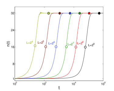
Figure 2: (Color online) Evolution of $n(t)$ for a population of $N=32$ agents on six different lattices of size $L=2^{m}$, $m=4,\ldots,9$. Full circles denote the Population-Awareness Times, empty circles the Outbreak Times.

This section is divided into three parts. The first considers only $n(t)$, the total informed population at time $t$, and the results presented are independent of the population distribution on levels. The second section takes into account the distribution on levels $n(l,t)$. The third section deals with the final information $\mathcal{I}(z)$. All the results are averaged over 500 different realizations of the system.

III.1 Level-independent results

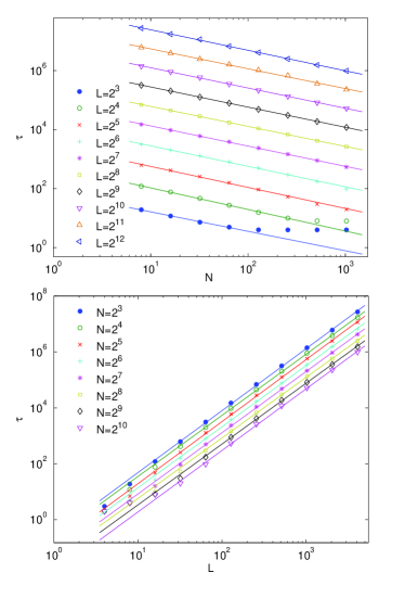
Figure 3: (Color online) Dependence of the Population-Awareness Time $\tau$ on the number of agents $N$ and the lattice size $L$. Top: Log-log scale plot of $\tau$ versus $N$; different lattice-size values are shown with different symbols and colors. For sufficiently small densities ($\rho\leq 1$), straight lines represent the best fit according to Eq. 4. Bottom: Log-log scale plot of $\tau$ versus $L$; different values of the number of agents are shown with different symbols and colors. Provided that the density $\rho$ is not large ($\rho\leq 1$), data points lay on the curves given by Eq. 4 which represent the best fit. Error on data points is $<2\%$.

Fig. 2 shows the typical time evolution of $n(t)$, the number of aware people at time $t$, for fixed $N$ and several different values of $L$. Due to the fact that, once informed, an agent can not modify his status, $n(t)$ is a monotonic increasing function. The curve is sigmoidal: $n(t)$ initially increases with an increasing growth rate $dn(t)/dt$. The growth rate is maximum at the Outbreak Time $t_{out}$, when usually $n(t_{out})\sim N/2$ (in Sec. IV we will justify this fact in a low-density approximation). The growth rate then begins to decrease; the evolution slows down and the curve begins to saturate. The information reaches all the population at the Population-Awareness Time $\tau$, that is the quantity that we analyze here (roughly $\tau\sim 2t_{out}$, and this fact as well will be justified in Sec. IV).

The Population-Awareness Time $\tau$ depends on the total number of agents $N$ and on the size of the lattice $L$, as shown in Fig. 3. As long as the density is not large ($\rho\leq 1$), data points are well fitted by power laws holding over a wide range (though logarithmic corrections can not be ruled out):

$$\tau\sim N^{-\alpha},$$ (2)

$$\tau\sim L^{\beta}.$$ (3)

The exponents $\alpha$ and $\beta$ are constant by varying $L$ or $N$, respectively, so that we can write:

$$\tau\sim N^{-\alpha}\,L^{\beta}.$$ (4)

The fitting of data with an asymptotic least-squares method yields the following exponents:

$$\alpha=0.68\pm 0.01\hskip 12.91663pt\beta=2.22\pm 0.03.$$ (5)

III.2 Level-dependent results

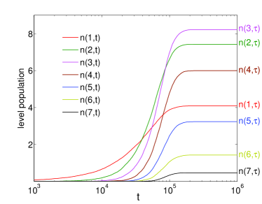
Figure 4: (Color online) Time evolution of level populations $n(l,\,t)$ for $N=32$, $L=512$.

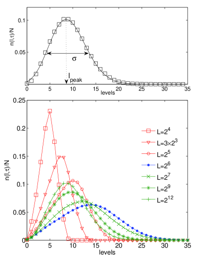
Figure 5: (Color online) Top: typical population distribution on levels at $t=\tau$ for a low-density system (N=1024, L=4096). Squares are experimental results; the line is the result of data fitting according to Eq. (6). Bottom: population distribution on levels at $t=\tau$ for systems with $N=1024$ and $L$ between $2^{4}$ and $2^{12}$ (the lines are guides to the eye): the behavior of the distribution is non-monotonic with respect to $L$. By increasing $L$ from small values, the curves first shift to the right and flatten ($L=16$, 24, 32). The rightmost, extremal curve corresponds to $L=64$. Then, by increasing $L$ the curves shift back to the left and sharpen ($L=128$, 512, 4096).

We now focus on the time evolution of $n(l,\,t)$, the population of level $l$. Each population evolves in time with a sigmoidal law (Fig. 4), with its own Outbreak Time and tending to a final value $n(l,\,\tau)$.

The final distribution of agents on levels $n(l,\,\tau)$ as a function of $l$ (Fig. 5, top) has an asymmetrical-bell shape, with a peak at position $l_{peak}$ and a width $\sigma$, both depending on $N$ and $L$ (notice that only a fraction of the $N$ available levels has a non-negligible population). If $L$ is large enough (larger than $\tilde{L}$, see below), the population distribution on levels is well fitted by the $3$-parameter function

$$\frac{n(l,\tau)}{N}=A\,\frac{\left(\mathrm{log}N\right)^{l}}{\Gamma(B\cdot l+C)},$$ (6)

where $\Gamma(x)$ is the Euler gamma function, and the parameters $A,B,C$ depend smoothly on $N$ and $L$. The fitting function is a generalization of Eq. (20), the distribution function of the low-density regime.

In Fig. 5, bottom, we show how the distribution $n(l,\,\tau)$ changes with $L$ for a fixed value $N=1024$ and we introduce one of the most important results of this paper. For $L$ small (hence for high density, $\rho\gg 1$) the distribution is very sharp and peaked on small values of $l$. As $L$ grows, the distribution shifts to higher values of $l$ and becomes more and more spread ($l_{peak}$ and $\sigma$ grow). The extremal, maximum-spread distribution is obtained for a value $L=\tilde{L}$ (for $N=1024$, $\tilde{L}\sim 64$): $l_{peak}$ and $\sigma$ are maximum; the highest possible number of levels is occupied. As $L$ is increased beyond $\tilde{L}$, the curve begins to shift back to smaller $l$s and to narrow; this process continues up to the low-density regime ($\rho\ll 1$). In general, $\tilde{L}$ depends on $N$.

The same phenomenon occurs if we keep $L$ fixed and let $N$ vary. By increasing $N$ from small, low-density values, the distribution shifts to the right and spreads, up to an extremal form occurring for $N=\tilde{N}$ (depending on $L$). Then, it shifts back and narrows.

This behavior has strong consequences on the efficiency of information spreading on the lattice, as we will see in the next section.

III.3 Degree of Information

In this section we deal with the final degree of information at the Population-Awareness Time, $\mathcal{I}(z)=\mathcal{I}(\tau,z)$ (in particular, with its average value $\mathcal{I}_{av}(z)=\mathcal{I}(z)/N$), and its dependence on $N$, $L$, and $z$. We remind (Eq. (1)) that $\mathcal{I}(z)$ is the generating function of the final populations $n(l,\,\tau)$, hence its value depends on the final distribution of the population on levels analyzed in the previous paragraphs.

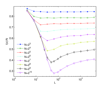
Figure 6: (Color online) Semilog scale plot of final degree of information per agent $\mathcal{I}_{av}(z)=\mathcal{I}(z)/N$ vs lattice size $L$. Several values of $N$ are shown with different symbols and colors (lines are guides to the eye), while the decay constant is fixed at $z=0.9$. Notice the occurrence of minima at $\tilde{L},\tilde{N}$, and that $\tilde{L}$ is monotonically increasing with respect to $\tilde{N}$. Error on data points is $<1.5\%$.

Once $z$ is fixed, $\mathcal{I}_{av}(z)$ depends nonmonotonically on $N$ and $L$; let us follow it for $N$ fixed and varying $L$ in Fig. 6. For $L$ small, due to the narrow distribution discussed in the previous section, the value of the information is high. When $L=\tilde{L}$, the population distribution on levels reaches its extremal form and the information displays a minimum. As $L$ increases, the information starts to rise again. So, the main result is that, given a population number $N$, there is an optimal lattice size $\tilde{L}$ for which the final information is minimum; this value is typically intermediate between the high-density and low-density regimes. The same happens having fixed $L$ and letting $N$ vary: there is a minimum for $N=\tilde{N}$, where $\tilde{N}$ depends on $L$.

This result implies that choosing an optimization strategy for the spreading of information on the lattice is not trivial. Suppose e.g. that we are given $N$ agents on a lattice and we want to maximize the final average information $\mathcal{I}_{av}(z)$ by varying the lattice size $L$ (starting from some $L_{0}$). This optimization process is meant to be local: we are not allowed to modify the size by several orders of magnitude, but just around the starting size $L_{0}$. Then, the choice whether to shrink or expand the lattice depends on $L_{0}$. If $L_{0}<\tilde{L}$, increasing $L$ takes the system closer to the information minimum ($\mathcal{I}_{av}(z)$ decreases); decreasing $L$ increases $\mathcal{I}_{av}(z)$ and is the right strategy. If on the other hand $L_{0}>\tilde{L}$, increasing $L$ is the right strategy.

Fig. 7 shows that the depth of the information minimum depends in turn on the decay constant $z$: as $z$ is varied from $0$ to $1$, there are some curves (corresponding to in-between values) which display a more emphasized minimum.

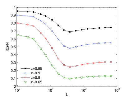
Figure 7: (Color online) Semilog scale plot of final degree of information per agent $\mathcal{I}_{av}(z)$ as a function of the lattice size $L$, when $N=2^{9}$ (lines are guides to the eye). Four different values of decay constant $z$ are considered, as shown by the legend.

Finally, in Fig. 8 we show how the final average degree of information $\mathcal{I}_{av}(z)$ depends on $z$, for different values of $N$, once the size $L$ is fixed. There are, as expected, two fixed points: when $z=1$ ($z=0$), $\mathcal{I}_{av}(z)$ is equal to $1$ ($0$), irrespective of the parameters ($N,L$) of the system. The function $\mathcal{I}_{av}(z)$ cannot be determined but in two particular regimes (low- and high-density).

When $\rho=N/L^{2}$ is sufficiently low ($\rho<2^{-8}$), the function is well fitted by

$$\mathcal{I}_{av}(z)=N^{z-1},$$ (7)

within the error ($<3\%$). When $\rho>1$, $\mathcal{I}_{av}(z)$ is fitted by

$$\mathcal{I}_{av}(z)=A\cdot z\rho\frac{(1-z^{B\cdot L})^{2}}{(1-z)^{2}},$$ (8)

with $A$, $B$ depending on $N$, $L$.

The two laws come from particular population distributions, as will be explained in the next section.

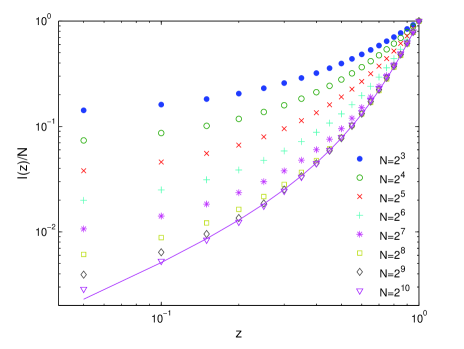
Figure 8: (Color online) Final ($t=\tau$) degree of information per agent $\mathcal{I}_{av}(z)$ versus the decay constant $z$. The size of the lattice is fixed as $L=2^{4}$, while several values of $N$ are considered and represented in different colors and symbols. The curve depicted is the best fit when $N=2^{10}$ ($\rho>1$), according to Eq. 8. Notice the existence of the fixed points $z=0$, $\mathcal{I}_{av}(z)=\frac{1}{N}$ and $z=1,\mathcal{I}_{av}(z)=1.$

IV Analytical Results

Consider a system with $N$ and $L$ fixed. Let $\mathcal{P}(t)$ be the probability that at time $t$ an unaware agent is in contact with at least 1 informed agent. Let $\mathcal{P}_{l}(k,s;\,t)$ be the probability that at time $t$ an unaware agent is in contact with $k+s$ informed agents, of which $k$ belonging to level $l$ and $s$ belonging to some other level. Then the evolution of the system is governed by two master equations, one for the total population:

$$n(t+1)=n(t)+(N-n(t))\,\mathcal{P}(t),$$ (9)

and one for the level populations:

$$n(l,\,t+1)=n(l,\,t)+(N-n(t))\sum_{k,s}\mathcal{P}_{l-1}(k,s;\,t)\frac{k}{k+s}.$$ (10)

$\mathcal{P}(t)$ and $\mathcal{P}_{l}(k,s;\,t)$ are very complex functions of their arguments and cannot be calculated in the general case. For example, $\mathcal{P}(t)$ depends not only on the number of informed agents $n(t)$ but also on their spatial distribution, hence on the instant and the site where each of them has been informed (in other words, on the history of the system). We will calculate the evolution of the system in two particular cases, for high and low densities, and finally compare the results with intermediate systems.

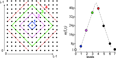
Figure 9: (Color online) Evolution of the system in the high-density approximation for a lattice with $L=12$ and a Source starting in the site with coordinates $(7,\,7)$. Left: the wave front of information on the lattice at times $t=1$, 2, 3, 4 has a square shape. Agents in the interior of the square are informed, agents on the exterior are unaware. Times correspond to levels: agents between the front at time 3 and that at time 4 belong to level 4, and so on. Right: final distribution of agents on levels; broken lines highlight the triangular shape of the distribution.

High-density regime. In this case ($\rho\rightarrow\infty$) there are many agents on every site. If the agents on a site get informed at a time $t$, we can suppose that at $t+1$ at least one of them will jump on each of the four nearest- neighbor sites: hence, all the unaware agents on the nearest- and next-to-nearest-neighbor sites will get information at time $t+1$. In this way (Fig. 9) information spreading among agents amounts to propagation of information through the lattice. A “wave front” of information travels with constant velocity: on the interior sites are informed agents, on the exterior sites unaware agents. If we suppose the Source to be at the center of the lattice at $t=0$, at each instant the wave front is the locus of points whose chemical distance from the center is $2t+1$. Consequently, $n(t)=\rho(8t^{2}-4t+1)$, up to the half-filling time $t_{out}\sim L/4$, when the front reaches the boundary of the lattice; for $t>L/4$, the equation is $n(t)=\rho(-8t^{2}+4t(2L+1)+(L+1)^{2})$. The Population-Awareness Time is $\tau\sim L/2$.

Almost all the agents on the wave front at time $t$ have received information at time $t-1$: so, each new time step adds a new level, whose population never changes at successive times. The population $n(l,\,t)$ is proportional to the length of the wave front at the time $t=l$: $n(l,\,t)\sim 4\rho(4l+1)$ up to $t=L/4$ and $n(l,\,t)\sim 4\rho(-4l+2L-1)$ up to $t=L/2$. As can be seen from Fig. 9, the shape of the level distribution at $t=\tau$ is triangular (compare this to the distribution for $L=16$ in Fig. 5). The Final Information is proportional to $\rho$, according to the formula

$$\mathcal{I}(z) =\sum_{l=0}^{N}n(l,\,\tau)z^{l}\sim\sum_{l=0}^{L/4}16\rho\,lz^{l}+\sum_{l=L/4+1}^{\tau}4\rho(2L-4l)z^{l}$$ (11)

$$=16z\rho\frac{(1-z^{L/4})^{2}}{(1-z)^{2}}.$$

A modified version of this equation, Eq.(8), has been used to fit the information curves for high-density regimes.

Low-density regime. In the case of low density ($\rho\ll 1$) the time an informed agent walks before meeting an unaware agent becomes very large. We can then assume that the agents between each event have the time to redistribute randomly on the lattice, that is, we adopt a mean-field approximation. Let $p=5/L^{2}$ be the probability that two given agents, randomly positioned on the lattice, are in contact (5 is the number of points contained in a circle of radius 1). Hence, $(1-p)^{n(t)}$ is the probability for an agent at time $t$ of not being in contact with any of the $n(t)$ informed agents, and $\mathcal{P}(t)=1-(1-p)^{n(t)}$ is the probability of being in contact with at least one informed agent. Master equation (9) becomes:

$$n(t+1)=n(t)+\left(N-n(t)\right)\left(1-(1-p)^{n(t)}\right),$$

and to first order in $p$:

$$n(t+1)=n(t)+p\,\left(N-n(t)\right)\,n(t).$$ (12)

Thus, $n(t+1)=f(n(t))$: $f$ is a logistic-like map, with a repelling fixed point in $0$ ($f^{\prime}(0)=1+Np$), and an attracting fixed point in $N$ ($f^{\prime}(N)=1-Np$). Since $Np=5\rho\ll 1$, the increment of $n(t)$ at each time step is very small (of order $p$), and we can take the evolution to be continuous. The equation becomes:

$$n(t+1)-n(t)\sim\frac{dn(t)}{dt}=p\,(N-n(t))\,n(t)$$ (13)

and the solution, with the initial condition $n(0)=1$, is the sigmoidal function

$$n(t)=N\frac{e^{Npt}}{e^{Npt}+N-1}.$$ (14)

The outbreak time, i.e. the flex of the curve, is in $t_{out}=\frac{\mathrm{log}(N-1)}{Np}$, that is also the half-filling time, $n(t_{out})=N/2$. The total population $N$ is reached only for $t=\infty$, but we can take the PAT to be the time when $N-1$ agents have been informed:

$$\tau=\frac{2\,\mathrm{log}(N-1)}{Np}\sim\frac{2\,\mathrm{log}N}{Np}\sim\frac{\mathrm{log}N}{N}L^{2},$$ (15)

where the last result holds for $N$ large: hence, in the low-density approximation the exponent for $L$ is $\beta=2$, while the law for $N$ contains logarithmic corrections and the exponent $\alpha$ cannot be defined. The first result in Eq. (15) shows that in this approximation $\tau=2\,t_{out}$.

The quantity $\mathcal{P}_{l}(k,s;\,t)$ in Eq. (10) is:

$$\mathcal{P}_{l}(k,s;\,t)= \left(\begin{array}[]{c}n(l,t)\\ k\end{array}\right)\left(\begin{array}[]{c}n(t)-n(l,t)\\ s\end{array}\right)$$

$$\times p^{k+s}(1-p)^{n(t)-(k+s)}.$$

The sum over $k$ and $s$ in Eq. (10), using the Chu-Vandermonde identity for binomial coefficients vandermonde , yields a master equation for the level populations in the mean-field approximation:

$$n(l,\,t+1)=n(l,\,t)+(N-n(t))(1-(1-p)^{n(t)})\frac{n(l-1,\,t)}{n(t)},$$

and to first order in $p$:

$$n(l,\,t+1)=n(l,\,t)+p\,n(l-1,\,t)\,(N-n(t)).$$

Its continuous version is:

$$\frac{dn(l,\,t)}{dt}=p\,n(l-1,\,t)(N-n(t))$$ (17)

that has to be solved for each $l$. For $l=1$, with the initial condition $n(1,\,0)=0$, we get the solution

$$n(1,\,t) =Np\,t-\mathrm{log}\left(e^{Np\,t}+N-1\right)+\mathrm{log}N$$

$$=\mathrm{log}\left(n(t)\right).$$

We then plug this solution into Eq. (17) to get $n(2,\,t)$, and so on. It can be shown by induction that for every $l$, with the initial condition $n(l,\,t)=0$,

$$n(l,\,t) =\frac{1}{l!}\left(Np\,t-\mathrm{log}\left(e^{Np\,t}+N-1\right)+\mathrm{log}N\right)^{l}$$ (18)

$$=\frac{1}{l!}\left(n(1,\,t)\right)^{l}=\frac{1}{l!}\left[\mathrm{log}\left(n(t)\right)\right]^{l}.$$

This set of curves (not shown here) is similar to that of Fig. 4, with crossovers and different Outbreak Times.

The normalized level population at each $t$ is:

$$\frac{n(l,\,t)}{n(t)}=\frac{1}{n(t)}\frac{1}{l!}\left[\mathrm{log}\left(n(t)\right)\right]^{l}=\frac{e^{-\mathrm{log}\left(n(t)\right)}\left[\mathrm{log}\left(n(t)\right)\right]^{l}}{l!},$$ (19)

hence, it is a Poisson distribution with mean $\mathrm{log}\left(n(t)\right)$.

The population distribution on levels at $t=\tau$ is

$$n(l,\,\tau)=\frac{\left(\mathrm{log}N\right)^{l}}{l!},$$ (20)

independent of $p$ (hence of $L$). A modified version of this distribution, Eq. (6), has been used to fit the numerical curves.

The total information is

$$\mathcal{I}(t,\,z) =\sum_{l=0}^{N}n(l,\,t)z^{l}=\sum_{l=0}^{N}\frac{1}{l!}\left[\mathrm{log}\left(n(t)\right)\cdot z\right]^{l}\sim$$ (21)

$$\sim e^{\mathrm{log}\left(n(t)\right)\cdot z}=n(t)^{z}.$$

In particular, $\mathcal{I}(\tau,\,z)=N^{z}$, in agreement with Eq. (7).

Figure 10: Snapshots of four systems with $N=1024$ and $L=16$, 32, 64, 512, all at an instant near to the half-filling time. Only informed agents are shown; they are represented as circles of radius 1. Notice that the high-density picture of a connected set of informed agents holds up to $L=\tilde{L}=64$. For $L\geq 64$, the picture breaks down and the system is better described by a low-density approximation ($L=512$).

In conclusion, we have examined the system in two different regimes, both optimal for information spreading. The worst case for information spreading, at $\tilde{L}$, seems to correspond to crossover between these two regimes, as shown in Fig. 10.

V Conclusions and perspectives

We have presented a model of information spreading amongst diffusing agents. The model takes into account a population made up of agents who are socially, as well as geographically, dynamic. Moreover, it allows for possible alteration of information occurring during the transmission process, by introducing a decay constant $z$.

Investigations are lead both by means of numerical simulations and of analytical methods valid in the high- and low-density regimes.

The main results are two. First: the time it takes the piece of information to reach the whole population of $N$ agents, distributed on a lattice sized $L$, depends on $N$ and $L$ according to a power law. This behavior holds over a wide range, where exponents are found to be constant and noninteger. Second: the final ($t=\tau$) average degree of information $\mathcal{I}_{av}(z)$ for a fixed population $N$ (lattice size $L$) shows a surprisingly non-monotonic dependence on the lattice size $L$ (on the population $N$), with the occurrence of a minimum. This means that, from an applied perspective, an optimization strategy for $\mathcal{I}_{av}(z)$ is possible with respect to $N$ and $L$.

Extensions of our model to networks embedded in topologically different spaces are under study.

References

- (1) S. Bornholdt and H. G. Schuster eds., Handbook of graphs and networks (Wiley-VCH, Berlin, 2003).
- (2) M. Llas, P.M. Gleiser, J.M. López and A. Díaz-Guilera, Phys. Rev. E 68, 66101 (2003) .
- (3) S.M. Hedetniemi, S.T. Hedetniemi and A. Liestman, Networks 18, 129 (1988).
- (4) Y. Moreno, M. Nekovee and A.F. Pacheco, Phys. Rev. E 69, 66130 (2004).
- (5) X. Guardiola, A. Díaz-Guilera, C.J. Pérez, A. Arenas and M. Llas, Phys. Rev. E 66, 26121 (2002).
- (6) Brajendra K. Singh and Neelima Gupte, Phys. Rev. E 68, 66121 (2003).
- (7) S. Eubank et al., Nature 429, 180 (2004).
- (8) A. Rapoport, Bull. Math. Biophys. 15, 523 (1953).
- (9) B. Allen, J. Math. Soc. 8, 265 (1982).
- (10) S.P. Borgatti, Soc. Net. 27, 55 (2005).
- (11) Zhongzhu Liu, Jun Luo and Chenggang Shao, Phys. Rev. E 64, 46134 (2001).
- (12) Luis López and Miguel A.F. Sanjuán, Phys. Rev. E 65, 36107 (2002).
- (13) R. M. Anderson, Population Dynamics of Infectious Diseases: Theory and Applications (Chapman and Hall, New York, 1982). For a more recent review see H. W. Hethcote, SIAM Review, 42, 599 (2000).
- (14) see e.g. http://mathworld.wolfram.com/Chu-VandermondeIdentity.html.