Fermion nodes and nodal cells of noninteracting and interacting fermions

Abstract

A fermion node is subset of fermionic configurations for which a real wave function vanishes due to the antisymmetry and the node divides the configurations space into compact nodal cells (domains). We analyze the properties of fermion nodes of fermionic ground state wave functions for a number of systems. For several models we demonstrate that noninteracting spin-polarized fermions in dimension two and higher have closed-shell ground state wave functions with the minimal two nodal cells for any system size and we formulate a theorem which sumarizes this result. The models include periodic fermion gas, fermions on the surface of a sphere, fermions in a box. We prove the same property for atomic states with up to $3d$ half-filled shells. Under rather general assumptions we then derive that the same is true for unpolarized systems with arbitrarily weak interactions using Bardeen-Cooper-Schrieffer (BCS) variational wave function. We further show that pair correlations included in the BCS wave function enable singlet pairs of particles to wind around the periodic box without crossing the node pointing towards the relationship of nodes to transport and many-body phases such as superconductivity. Finally, we point out that the arguments extend also to fermionic temperature dependent/imaginary-time density matrices. The results reveal fundamental properties of fermion nodal structures and provide new insights for accurate constructions of wave functions and density matrices in quantum and path integral Monte Carlo methods.

I Introduction

Let us consider a system of fermions described by a real wave function $\Psi(R)$ where $R$ denotes fermions coordinates $R=({\bf r}_{1},...,{\bf r}_{N})$. Due to the antisymmetry, there exists a subset of fermion configurations for which the wave function vanishes and this subset is called the fermion node. The fermion node can be implicitly defined by $\Psi(R)=0$, assuming that the nodal set does not include configurations for which the wave function vanishes because of other reasons, eg, boundary conditions. In general, for $N$ spin-polarized fermions in a $d$-dimensional space, the fermion node is a $(dN-1)-$dimensional manifold (hypersurface). It is a well-known fact that for $d>1$ the antisymmetry alone does not specify fermion nodes completely. This is not difficult to understand since antisymmetry fixes only lower-dimensional coincidence hyperplanes with dimensionalities $(dN-d)$. Therefore the fermion nodes and their properties are determined by interactions and many-body effects.

The fermion nodes play an important role in quantum Monte Carlo (QMC) methods which belong to the most promising and productive approaches for studying quantum many-body systems. Let us briefly describe the basic idea of QMC and its relationship to fermion nodes. Consider a Hamiltonian $H$ and a trial function $\Psi_{T}(R)$ which approximates the ground state $\Psi_{0}(R)$ of $H$ within a given symmetry sector. It is straightforward to show that $\lim_{\tau\to\infty}\exp(-\tau H)\Psi_{T}\propto\Psi_{0}$ where $\tau$ is a real parameter (imaginary time). This imaginary time projection can be conveniently carried out by simulating a stochastic process which maps onto the imaginary time Schrödinger equation. The wave function is represented by an ensemble of $R$-space sampling points which are propagated according to $G(R,R^{\prime},\tau)=\langle R|\exp(-\tau H)|R^{\prime}\rangle$ and for large $\tau$ the ensemble becomes distributed according to $\Psi_{0}$. Unfortunately, the straightforward application of this idea to fermionic systems encounters a fundamental complication in the fermion sign problem qmchistory ; hammond ; jbanderson . The fermion sign problem makes QMC studies of large fermionic systems difficult since the statistical errors of fermionic expectation values grow exponentially in the projection time $\tau$ and also in the number of particles $N$.

One possibility for avoiding the fermion sign problem is to employ the fixed-node approximation which restricts the fermion node of the solution $\Psi_{0}(R)$ to be identical to the fermion node of an appropriate trial function $\Psi_{T}(R)$. The fixed-node approximation introduces an energy bias which scales as the square of the difference between the exact and approximate nodes and therefore the accuracy of fermion nodes becomes very important. In particular, for the exact node one can obtain the exact energy in computational time proportional to a low-order polynomial in $N$. The fixed-node approximation has been very successful even for rather approximate nodes of commonly used trial wave functions which are based on Hartree-Fock (HF) determinants or a few-determinant post-HF expansions. The fixed-node QMC electronic structure calculations using HF or post-HF nodes usually recover between 90 and 95 % of the correlation energy and energy differences agree with experiments typically within a few percent. Such encouraging results have been observed across many systems such as atoms, molecules, clusters and solids qmcrev . It is remarkable that QMC methods have enabled us to ”corner” the correlation energy problem into the last few percent of the correlation energy using algorithms which polynomial scaling.

Unfortunately, for many problems even a few percent of the correlation energy can be significant. Typical examples are transition metal systems where the fixed-node error can be of the order of several eVs. It is therefore clear that better understanding of fermion nodes could be an important step forward for the QMC methodology and beyond. In addition, the fermion nodes are related to other physical quantities and could shed light on other many-body phenomena which currently are not completely understood.

In order to introduce the basic properties of the fermion nodes and to illustrate the problems involved we will first mention a few unique cases of interacting systems for which the nodes are known exactly. These examples include a few two- and three-electron atomic states, namely, triplets of He atom ${}^{3}S(1s2s)$, ${}^{3}P(2p^{2})$ dariohe and the exact node of a three-electron atomic state ${}^{4}S(p^{3})$ bajdichnode . The wave functions of these high symmetry states can be parametrized by appropriate coordinate maps in which the node is described by a single variable. For example, in the case of He triplet ${}^{3}S(1s2s)$ state the corresponding ”nodal coordinate” is $\cos\beta={\bf r}^{+}_{12}\cdot{\bf r}_{12}/(r^{+}_{12}r_{12})$ where ${\bf r}^{+}_{ij}={\bf r}_{i}+{\bf r}_{j}$, ${\bf r}_{ij}={\bf r}_{i}-{\bf r}_{j}$. For the triplet ${}^{3}P(2p^{2})$ the relevant variable is $\cos\omega^{\prime}={\bf z}_{0}\cdot({\bf r}_{1}\times{\bf r}_{2})$ assuming that the $P$ state is oriented along the $z$-axis which is specified by the unit vector ${\bf z}_{0}$ dariohe ; bajdichnode . For the quartet state ${}^{4}S(p^{3})$ the node is captured by the variable $\cos\omega={\bf r}_{1}\cdot({\bf r}_{2}\times{\bf r}_{3})$. The node in these systems is encountered whenever the corresponding variable, $\cos\beta,\cos\omega^{\prime}$ or $\cos\omega$, vanishes.

The nodal surface divides the space of fermion configurations into nodal cells, sometimes also called domains. (The name nodal cell was introduced in the previous paper davidnode . In algebraic geometry and topology nodal cells are usually called nodal domains, see, for example, Ref. berger . We will use both of these two expressions interchangeably.) The few known examples of exact nodes mentioned in the preceding paragraph help to illustrate an important point, which has been conjectured for the fermionic ground states for some time davidnode , namely, that the ground state node divides the configuration space into the minimal number of two nodal cells: a ”plus” cell with $\Psi>0$ and a ”minus” cell with $\Psi<0$. From the node equation $\cos\beta=0$ of the ${}^{3}S(1s2s)$ state we easily find that the ”plus” and ”minus” domains are given by the conditions $r_{1}>r_{2}$ and $r_{1}<r_{2}$, respectively. For the node given by $\cos\omega^{\prime}=0$ the nodal domains are given by the orientation of ${\bf z}_{0},{\bf r}_{1},{\bf r}_{2}$: the three vectors are either left- or right-handed, corresponding to either ”plus” or ”minus” cell, respectively. Similarly, for the node $\cos\omega=0$ the domains are given by the left- or right-handedness of the vectors ${\bf r}_{1},{\bf r}_{2},{\bf r}_{3}$. The minimal number of two nodal domains was found also for $2D$ and $3D$ noninteracting spin-polarized homogeneous electron gas with periodic boundary conditions for up to 200 particles using a numerical proof davidnode .

Understanding the fermion nodes and their properties has become a challenge which might help to advance both practical calculations but also open a deeper insights into the properties of fermionic systems. One can envision two key problems:

a) Topology of the fermion nodes, ie, how many nodal cells are actually present since this is of high importance for the fixed-node QMC approaches. Note that if the number of nodal cells is incorrect (typically higher than it should be since mean-fields such as HF have tendency to divide the configurations space into too many domains) then the QMC sampling around the artificial nodes will be very sparse. This could lead to large statistical fluctuations from poor sampling, and, possibly, to an effective non-ergodicity due to the finite-time projection time in practical calculations.

b) Once the topology is correct, the accuracy of the manifold shape becomes important. This is an area where our insights are particularly limited since the exact nodes for large interacting systems are virtually unknown except for a few-particle special cases mentioned above.

In our recent paper mitasshort , we have made some encouraging steps forward in trying to understand the topological issues and we have analytically derived a number of new results regarding the number of nodal domains. In particular, we have shown that spin-polarized closed-shell ground states of noninteracting harmonic fermions in $d=2$ and higher have the minimal number of two nodal domains. We have proved the same for spin-polarized atomic states with several electrons, both for noninteracting and HF wave functions. We have also shown that by imposing additional symmetries one can generate more than two nodal domains but that interactions can relax this ”nodal degeneracy” to the minimal number of two domains such as in the case of the ${}^{4}S(1s2s3s)$ atomic state.

For noninteracting spin-unpolarized systems, ie, with both spin channels occupied, the number of nodal cells is four since the wave function is a product of spin-up and spin-down Slater determinants ($2\times 2=4$). (Here and later on we assume that the Hamiltonian does not include spin-dependent terms so that the particle spins are conserved. The wave function is then a product of two determinants which depend only on the spatial degrees of freedom qmcrev .) In the last few years, studies of a few-particle systems have revealed that interactions and many-body effects do affect the nodal topologies and can change the number of nodal cells dariobe ; cmt28 . In particular, for the case of Be atom it has been found that the noninteracting/HF four nodal cells of the singlet ground state change to the minimal number of two due to the electron correlation dariobe and qualitatively the same has been observed in other systems cmt28 . In our recent paper mitasshort we have found that this is a rather generic property of ground states in interacting systems. With some conditions, we have explicitly demonstrated that interactions lift the ”nodal cell degeneracy” in spin-unpolarized systems and smooth out the four noninteracting cells into the minimal two. We have shown this for $2D$ harmonic fermions in closed-shell states of arbitrary size using a variational Bardeen-Cooper-Schrieffer wave function.

In this work we further advance these ideas. We analyze the fermion nodes in a number of other paradigmatic fermionic models: homogeneous electron gas with periodic boundary conditions, particles in an infinite well and on the surface of a sphere. For all these systems we prove that in the spin-polarized noninteracting closed-shell ground state the fermion nodes divide the configuration space into minimal two cells for arbitrary number of particles. We also extend our previous proof for spin-unpolarized systems demonstrating that interactions smooth out multiple nodal cells of noninteracting/mean-field wave functions into the minimal two for more systems such as homogeneous electron gas and $3D$ harmonic oscillator. These results contribute to our understanding of the fermion nodes and their impacts on the accuracy of wave functions with direct implications for the QMC methods.

In the last sections we show how in periodic spin-unpolarized interacting fermion gas the pairs of particles can wind around the box without crossing the node what points towards the connection of nodes to the transport and to the existence of other quantum phases such as superconductivity. Finally, we then generalize the results to the temperature density matrices with the implications for path integral Monte Carlo methods davidhe .

II II. General properties of fermion nodes.

Let us introduce the basic properties of fermion nodes as they were studied by Ceperley davidnode some time ago.

a) Nondegenerate ground states wave functions fulfill the so-called tiling property. Let us define a nodal cell $\Omega(R_{0})$ as a subset of configurations which can be reached from the point $R_{0}$ by a continuous path without crossing the node. The tiling property says that by applying all possible particle permutations to an arbitrary nodal cell one covers the complete configuration space. Note that this does not specify how many nodal cells are there.

b) If $m$ nodal surfaces cross then the angle of crossing is $\pi/m$. Furthermore, the symmetry of the node is the same as the symmetry of the state.

c) It is possible to show that there are only two nodal cells using the following argument based on triple exchanges. Let us first introduce the notion of particles connected by triple exchanges. We will call the three particles $i,j,k$ connected if there exists a triple exchange path $i\to j,j\to k,k\to i$ which does not cross the node. If more than three particles are connected then they can form a connected cluster. An example of six particles connected into a single cluster is sketched as follows: . If there exists a point $R_{t}$ such that all the particles are connected into a single cluster then $\Psi(R)$ has only two nodal cells. This can be better understood once we realize the following two facts. First, any triple permutation can be written as two pair permutations. Therefore the connected cluster of triple permutations enables to realize any even parity permutation without crossing the node. That exhausts all permutations which are available for cell of one sign since the wave function is invariant to even parity permutations. Second, the tiling property implies that once the particles are connected for $R_{t}$ the same is true for the entire cell. By symmetry, the same arguments apply to the complementary ”minus” cell which correspond to the odd permutations. More details on this property can be found in the original Ref. davidnode .

III III. Noninteracting spin-polarized fermions.

III.1 III.a. Homogeneous electron gas.

We consider a system of spin-polarized noninteracting fermions in a periodic box in $d$ dimensions. The spatial coordinates are rescaled by the box size so that we can use dimensionless variables and the box becomes $(-\pi,\pi)^{d}$.

We first analyze the fermion nodes for $d=1$ since the result will be useful in subsequent derivations. We consider a system with $N=(2k_{F}+1)$ particles. In our $1D$ dimensionless units the Fermi momentum becomes an integer, $k_{F}=1,2...$. The one-particle occupied states are written as $\phi_{n}(x)=e^{inx},$ $n=0,\pm 1,...,\pm k_{F}$ and the spin-polarized ground state is given by

$$\Psi_{1D}(1,...,N)={\rm det}\left[\phi_{n}(x_{j})\right]$$ (1)

where $x_{j}$ is the $j$-th particle coordinate and $j=1,...,N$. We factorize the term $\exp(-ik_{F}\sum_{j}x_{j})$ out of the determinant so that the Slater matrix elements become powers of $z_{j}=e^{ix_{j}}$. The resulting Vandermonde determinant can be written in a closed form and after some rearrangements we find

$$\Psi_{1D}(1,...,N)=e^{-ik_{F}\sum_{j}x_{j}}\prod_{j>k}(z_{j}-z_{k})=$$

$$=\mu_{0}\prod_{j>k}\sin(x_{jk}/2)$$ (2)

where $x_{jk}=x_{j}-x_{k}$ and $\mu_{0}$ is a constant prefactor which is unimportant for our purposes. (In the derivations below we will be using the letter $\mu$ for denoting prefactors which are either constants or nonnegative functions in particle coordinates and therefore do not affect the nodes). The derived wave function has the following important properties.

a) The fermion nodes appear at the particle coincidence points. This implies a well-known result that the ground state wave function in $1D$ have $N!$ nodal cells since any particle permutation requires crossing the node at least once. In addition, this also means that any fermion configuration which preserves the particle order is contained within the same nodal domain/cell.

b) The wave function is invariant to translations and cyclic exchanges of particles. Due to the periodic boundary conditions this includes also winding the system around the periodic box, ie, the translation of all particles by $2\pi$. We can formalize this by introducing an operator $T^{x}_{a}$ which translates all the particles along the $x$-axis as $x_{j}\to x_{j}+a$ so that the translation invariance can be written as

$$T_{a}^{x}\Psi_{1D}(1,...,N)=\Psi_{1D}(1,...,N)$$ (3)

Similarly, the wave function is invariant to cyclic exchange of all the particles given by $j\to j+1,j=1,...,N$ and $N+1\to 1$. This action is carried out by $C_{+1}^{x}$ operator where the notation means the exchange by one site is in the $+x$-direction. Clearly, the inverse operator $[C_{+1}^{x}]^{-1}=C_{-1}^{x}$. Note that here we have assumed that $N$ is odd, in agreement with our definition. The invariance holds only for $N$ odd since then the cyclic exchange is equivalent to an even number of pair exchanges. For the sake of completeness, we consider also $N$ even, when the cyclic exchange can be replaced by an odd number of pair exchanges, resulting in the wave function sign flip. In general, for the cyclic exchanges we can therefore write

$$C_{\pm 1}^{x}\Psi_{1D}(1,...,N)=(-1)^{N+1}\Psi_{1D}(1,...,N)$$ (4)

c) Assuming the particle positions are all distinct, the cyclic exchange path can be chosen in such a way that it does not cross the node. This is easy to accomplish by maintaining finite distances between the particles along the path trajectory. Let us parametrize the exchange path by a parameter $t$ so that the path starts at $t=0$, the path is completed at $t=1$ and the exchange path operator is then denoted as $C^{x}_{+1}(t)$ with $0\leq t\leq 1$. The fact that the path does not cross the node (ie, the path is contained within the same nodal cell) can be then written as

$$|C_{+1}^{x}(t)\Psi_{1D}(1,...,N)|>0,\;0\leq t\leq 1$$ (5)

where, of course, $N$ is assumed to be odd.

Let us now derive the wave functions and generalize the results for fermions in $2D$. The one-particle states in $2D$ are $\phi_{nm}(x,y)=e^{i(nx+my)}$. The states are occupied up to the Fermi momentum $k_{F}$ so that we have $n^{2}+m^{2}\leq k_{F}^{2}$, where $k_{F}$ in $2D$ is not necessarily an integer. Similarly to our previous paper mitasshort , we show that the spin-polarized electron gas for closed-shell ground states have only two nodal cells.

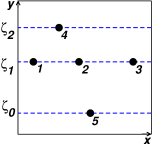
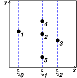
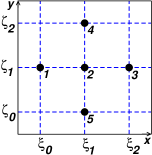
(a)	(b)	(c)

Figure 1: Positions of five fermions in the $2D$ periodic box $(-\pi,\pi)^{2}$. (a) Particles aligned horizontally, along the lines $y=\zeta_{0},\zeta_{1},\zeta_{2}$. (b) Particles aligned vertically, along the lines $x=\xi_{0},\xi_{1},\xi_{2}$. (c) Particles aligned in both directions, positioned on a lattice.

The proof is by induction, therefore let us first consider $k_{F}=1$ with five particles occupying $\{1,e^{\pm ix},e^{\pm iy}\}$ one-particle states. We place the particles as in Fig.1a so that the coordinates are given by ${\bf r}_{1}=(x_{1},\zeta_{1})$, ${\bf r}_{2}=(x_{2},\zeta_{1})$, ${\bf r}_{3}=(x_{3},\zeta_{1})$, ${\bf r}_{4}=(x_{3},\zeta_{2})$, ${\bf r}_{5}=(x_{5},\zeta_{0})$. By eliminating the terms with $\zeta_{1}$ the wave function can be factorized as follows

$$\Psi_{2D}(1,...,5)=\left|\begin{array}[]{ccccc}1&1&1&1&1\\ e^{ix_{1}}&e^{ix_{2}}&e^{ix_{3}}&e^{ix_{4}}&e^{ix_{5}}\\ e^{-ix_{1}}&e^{-ix_{2}}&e^{-ix_{3}}&e^{-ix_{4}}&e^{-ix_{5}}\\ e^{i\zeta_{1}}&e^{i\zeta_{1}}&e^{i\zeta_{1}}&e^{i\zeta_{0}}&e^{i\zeta_{2}}\\ e^{-i\zeta_{1}}&e^{-i\zeta_{1}}&e^{-i\zeta_{1}}&e^{-i\zeta_{0}}&e^{-i\zeta_{2}}\\ \end{array}\right|=$$

$$\mu_{0}\left|\begin{array}[]{ccc}1&1&1\\ e^{ix_{1}}&e^{ix_{2}}&e^{ix_{3}}\\ e^{-ix_{1}}&e^{-ix_{2}}&e^{-ix_{3}}\\ \end{array}\right|\left|\begin{array}[]{cc}e^{i\zeta_{0}}-e^{i\zeta_{1}}&e^{i\zeta_{2}}-e^{i\zeta_{1}}\\ e^{-i\zeta_{0}}-e^{-i\zeta_{1}}&e^{-i\zeta_{2}}-e^{-i\zeta_{1}}\\ \end{array}\right|=$$

$$=\mu_{0}^{\prime}\Psi_{1D}(1,2,3)\sin(\zeta_{10}/2)\sin(\zeta_{20}/2)\sin(\zeta_{21}/2)$$ (6)

where $\mu_{0},\mu_{0}^{\prime}$ are irrelevant constant prefactors. We have obtained a product of $1D$ wave function and terms with distances between the lines $y=\zeta_{0},\zeta_{1},\zeta_{2}$. Note that analogous result can be found for the configuration sketched in Fig. 1b so the particles are aligned in parallel to the $y$-axis with the wave function given by

$$\Psi_{2D}(1,...,5)=\mu_{0}\Psi_{1D}(5,2,4)\times$$

$$\times\sin(\xi_{10}/2)\sin(\xi_{20}/2)\sin(\xi_{21}/2)$$ (7)

If the particles are aligned in both directions as in Fig. 1c both expressions apply. From the derived wave function it is clear that the node is encountered when particles lying on the same line reorder or when the lines of particles cross each other, eg, $\xi_{1}=\xi_{0}$. The wave functions for the configurations outlined in Fig.1 possess an important property. Consider $\Psi_{1D}(...)$ in Eqs. 6, 7 with groups of particles positioned on the corresponding lines. Assuming the group of particles is allowed to move only along the given line, one can consider this to be an effective $1D$ subspace. The $1D$ wave function for such a subspace obeys all three conditions derived for $1D$ case, ie, Eqs. 3, 4 and 5. For example, for $\Psi_{1D}(1,2,3)$ which appears in Eq. 6 we have $|C_{+1}^{x}(t)\Psi_{1D}(1,2,3)|>0$. This is easy to check also analytically. We fix the coordinates in Fig.1(a) as follows $x_{1}=-2\pi/3,x_{2}=0,x_{3}=2\pi/3$ and then we can carry out a ”synchronized” cyclic exchange using the translation by $2\pi/3$ in $x$-direction. The wave function is constant along the translation/cyclic exchange path so that we have

$$C^{x}_{+1}(t)\Psi_{1D}(1,2,3)=\Psi_{1D}(1,2,3),\;\;0\leq t\leq 1$$ (8)

because of the translational invariance.

Finally, we are ready to show that there are only two nodal cells in this five-particle ground state. Assume that the particles are positioned as in Fig.1c. Consider the following sequence of four exchanges, $C^{x}_{+1}C^{y}_{+1}C^{x}_{-1}C^{y}_{-1}$, where the operators act from the right, ie, $C^{y}_{-1}$, acts first. We denote this exchange symbolically as

$$C_{\rightarrow\uparrow\leftarrow\downarrow}=C^{x}_{+1}C^{y}_{+1}C^{x}_{-1}C^{y}_{-1}$$ (9)

The exchanges are performed only for the particles lying on the lines $\zeta_{1},\xi_{1}$ in corresponding directions, eg, $C_{\pm 1}^{x}$ acts on particles along $y=\zeta_{1}$ while $C_{\pm 1}^{y}$ cycles particles along $x=\xi_{1}$ . It is easy to check that this results in a triple exchange $423\to 342$ while the particles 1 and 5 end up in their original positions. It is therefore clear that particles 2,3,4 are connected by this triple exchange. It is straightforward to show that $C^{x}_{-1}C^{y}_{-1}C^{x}_{+1}C^{y}_{+1}$ exchanges particles 1,2,5 so that we can conclude that all five particles are connected by triple exchanges into a single cluster and there are only two nodal domains.

Now we need to extend the arguments and find the wave functions for general cases with occupied states within the Fermi disk with an arbitrary $k_{F}$. It is instructive to first derive the wave functions for $k_{F}=\sqrt{2}$ with 9 particles occupying states $\{1,e^{\pm ix},e^{\pm iy},e^{i(\pm x\pm y)}\}$ and for $k_{F}=2$ with 13 particles with additional states $\{e^{\pm i2x},e^{\pm i2y}\}$. This will enable us to understand how to write down the wave function for a general case while avoiding rather tedious notations which would appear in the direct derivations.

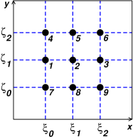
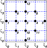
(a)		(b)

Figure 2: Positions of fermions in the $2D$ periodic box in real space. (a) Positions of the nine-fermion system. (b) Positions of the 13-fermion system. See the text for details.

Let us position the particles into a pattern which mimics the lattice of the occupied wave vectors in the reciprocal space, see Fig.2. Using appropriate algebraic arrangements we subsequently factorize the lines of particles as given by

$$\Psi_{2D}(1,...,9)=$$

$$=\mu_{0}\Psi_{1D}(1,2,3)\Psi_{2D}(4,...,9)\sin^{3}(\zeta_{21}/2)\sin^{3}(\zeta_{10}/2)=$$

$$=\mu_{0}^{\prime}\Psi_{1D}(1,2,3)\Psi_{1D}(4,5,6)\Psi_{1D}(7,8,9)\times$$

$$\times\sin^{3}(\zeta_{21}/2)\sin^{3}(\zeta_{10}/2)\sin^{3}(\zeta_{20}/2)$$ (10)

where $\mu_{0},\mu_{0}^{\prime}$ are constants. Similarly, for $k_{F}=2$ we can first factorize the line with the largest number of particles on $y=\zeta_{2}$ (see Fig.2)

$$\Psi_{2D}(1,...,13)=\mu_{0}\Psi_{1D}(1,...,5)\sin(\zeta_{02}/2)\sin^{3}(\zeta_{12}/2)\times$$

$$\times\sin^{3}(\zeta_{32}/2)\sin(\zeta_{42}/2)\Psi_{2D}(6,...,13)$$

and then factorize out the particles lying on another line $y=\zeta_{3}$ to obtain

$$\Psi_{2D}(1,...,13)=\mu_{0}\left[\prod_{j\neq 2}\sin^{n_{j}}(\zeta_{j2}/2)\right]\left[\prod_{j\neq 2,3}\sin^{n_{j}}(\zeta_{j1}/2)\right]\times$$

$$\Psi_{1D}(1,...,5)\Psi_{1D}(6,7,8)\Psi_{2D}(9,...,13)$$ (11)

where $n_{j}$ is the number of particles lying on the line $y=\zeta_{j}$. We have obtained a product of $1D$ wave functions, terms with distances between the lines and the $2D$ wave function with lower number of particles positioned in the same type of pattern is in Fig.1. Obviously, we can further factorize $\Psi_{2D}(9,...,13)$ using Eq.6 until we end up with $1D$ factors only. Using these insights into the recursive form of the wave function, for a general case with $M+1$ lines we can write

$$\Psi_{2D}(1,...,N)=$$

$$=\mu_{0}\prod_{k=0}^{M}\left[\Psi_{1D}(I_{k})\prod_{j>k}\sin^{n_{j}}(\zeta_{jk}/2)\right]$$ (12)

where $I_{k}=i^{(k)}_{1},...,i^{(k)}_{n_{k}}$ denotes the labels of particles lying on the line $y=\zeta_{k}$. In addition, analogous expression can be found if we factorize along the $x=\xi_{j}$ lines, the only difference being replacement $\zeta_{jk}$ by $\xi_{jk}$ and corresponding replacement of particle sets in $\Psi_{1D}$ wave functions.

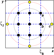
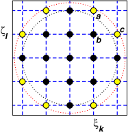
(a)		(b)

Figure 3: Illustrations of the position patterns in $2D$ periodic box for the size increases from $k_{F}$ to $k_{F}+\Delta k_{F}$. The particle layouts mimic the occupied states in the reciprocal space, however, the particles are positioned in the real space. The additional particles are in grey/yellow. (a) The additional particles positioned along $x-$ and $y-$axis directions. (b) The additional particles positioned along diagonals. Lines $x=\xi_{k}$ and $y=\zeta_{l}$ are used for the proof that the particles $a,b,c$ are connected by a triple exchange. See the text for details.

We are now ready for the induction step. Consider a spin-polarized closed-shell ground state with a given $k_{F}$. For this wave function we assume that all the particles are connected by the triple exchanges, ie, there are only two nodal domains. Let us increase $k_{F}\to k_{F}+\Delta k_{F}$ until the Fermi disk includes the next unoccupied star of states $\phi_{nm}(x,y)$ for which $k_{F}<(n^{2}+m^{2})^{1/2}\leq k_{F}+\Delta k_{F}$. The system size increases by the corresponding number of additional particles. Assuming the particles are positioned in the real space in the same pattern as the occupied ${\bf k}$-points in reciprocal space (Fig.3), the additional particles will appear at the borderline of the disk in the real space.

The two basic possibilities how the additional particles are positioned are given in the Fig.3. We need to show that these additional particles are connected to the original particles by the triple exchanges. This can be demonstrated by the sequence of the four cyclic exchanges which we have used above for the five particle case. It involves particles on the lines $x=\xi_{k}$ and $y=\zeta_{l}$ as schematically drawn in Fig.3. Consider the exchange $C_{\rightarrow\uparrow\leftarrow\downarrow}=$ $C^{x}_{+1}C^{y}_{+1}C^{x}_{-1}C^{y}_{-1}$ where the cyclic exchanges in $x$ direction are applied only to particles on the line $x=\xi_{k}$ and, similarly, the cyclic exchanges in $y$ direction are applied only to particles along $y=\zeta_{l}$. Note the wave function is invariant to cyclic exchanges since the number of particles along each line is odd for any closed shell state. It is then straightforward to find out that $C_{\rightarrow\uparrow\leftarrow\downarrow}$ exchanges particles $a,b,c$ while the rest of the particles remains intact. Similar exchanges can be carried out for all additional particles. Finally, this shows that the additional particles are connected to the particles of the wave function with size $k_{F}$ and finalizes the proof.

The proof can be extended into $3D$ and higher dimension by positioning the particles onto an appropriate $3D$ pattern which in real space mimics the occupied states in the Fermi sphere in the reciprocal space. This is possible due to the fact that with proper positioning of particles one can subsequently factorize the Slater determinant along hyperplanes, planes and lines. Using arguments similar to the $2D$ case we can perfrom cyclic exchanges without crossing the node in $3D$ and higher dimensions. Therefore the proof for higher dimensions is essentially the same.

In many cases, the proof can be extended to open shells. If an open-shell state is degenerate it is necessary to fix the ambiguity in the nodes, for example, by considering wave functions which transform according to an appropriate symmetry subgroup davidnode ; foulkes . In general, however, depending on symmetries, the number of degenerate states, etc, one cannot rule out possibilities of states with the number of cells beyond the minimal two (this will be investigated in the next paper).

This concludes the arguments and the proof that for $d>1$ the noninteracting spin-polarized fermion gas closed-shell ground states in periodic boundary conditions have only two nodal cells.

III.2 III.a. Fermions on the surface of a sphere.

Spin-polarized free fermions on the surface of a sphere are described by a Slater determinant with one-particle states being the spherical harmonics $Y_{lm}(\vartheta,\varphi)$. The spherical harmonics are polynomials in variables $\cos\vartheta$ and $\sin\vartheta e^{\pm i\varphi}$. The Slater matrix elements can be rearranged to monomials in these variables and it is then straightforward to factorize the determinant into similar form as obtained for the homogeneous fermion gas or for the harmonic oscillator mitasshort . Let us assume that the particles are positioned as sketched in Fig. 4a. Using familiar expressions for the first few spherical harmonics we get for the ${}^{5}S(sp^{3})$ state

$$\Psi_{sp^{3}}(1,...,4)=\mu_{0}(u_{1}-u_{0})v_{1}^{2}\prod_{2\leq i<j\leq 4}\sin(\varphi_{ij}/2)$$ (13)

where we have denoted $u=\cos\vartheta$ and $v=\sin\vartheta$ and $\mu_{0}$ is a constant. Similarly, for the ${}^{10}S(sp^{3}d^{5})$ state with nine fermions we obtain

$$\Psi_{sp^{3}d^{5}}(1,...,9)=\mu^{\prime}_{0}\Psi_{sp^{3}}(1,...,4)\times$$

$$\times(u_{2}-u_{0})(u_{2}-u_{1})^{3}v_{2}^{6}\Psi_{1D}(5,...,9)$$ (14)

where we have denoted $\Psi_{1D}(1,...,N)=\prod_{j<k}\sin(\varphi_{jk}/2)$ in agreement with Eq. 2.

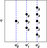
(a)		(b)

Figure 4: Positions of the particles on the sphere surface for the state ${}^{10}S(sp^{3}d^{5})$ using coordinate system $u=\cos(\vartheta)$ and $0\leq\varphi\leq 2\pi$. The particles are positioned along the lines with constant $u=u_{j}$. For larger systems the patterns are the same with particles corresponding to increasing angular momentum $l$ lying on the lines with increasing $u_{l}$. (a) Particle positions used for derivation of the wave function factorization. (b) Particles after appropriate shifts along $\varphi$ and a subsequent rotation.

For an arbitrary size closed-shell $S$ symmetry state the one-particle states are occupied up to the angular momentum $L$ with the corresponding number of particles $N=\sum_{l=0}^{L}(2l+1)=(L+1)^{2}$. Using the previous two examples we can directly write the factorized wave function assuming the particle positions follow the pattern in Fig. 4a. We first factorize the line $u=u_{L}$ and then recursively the rest of the lines so that we can write

$$\Psi(1,...,N)=\mu_{0}\Psi_{2D}(1,...,N/I_{L})\times$$

$$\times\Psi_{1D}(I_{L})v_{L}^{L(L+1)}\prod_{0\leq j<L}(u_{L}-u_{j})^{n_{j}}=$$

$$=\mu(v_{1},...,v_{L})\prod_{k=0}^{L-1}\left[\Psi_{1D}(I_{L-k})\prod_{j<L-k}(u_{L-k}-u_{j})^{n_{j}}\right]$$ (15)

where $I_{k}$ is the subset of particles lying on the line $u=u_{k}$. In the final expression the powers of $v_{j}$, such as $v_{L}^{L(L+1)}$ in the preceding line, are absorbed into $\mu(v_{1},...,v_{L})$. This prefactor is nonnegative and does not affect the nodes or the wave function rotational invariance.

We use the properties of $1D$ wave functions and the rotational invariance to build the proof of the two nodal domains. First, note that for four particles in ${}^{5}S(sp^{3})$ state it is easy to show mitasshort that there are only two domains. A little bit of algebra shows that the node is encountered when all four particles lie on a circle resulting from a plane cutting the sphere. Clearly, it is easy to position the four particles on the sphere so that the triple exchanges do not cross this node. For the induction step assume that for the size $L$ with $N=(L+1)^{2}$ the particles are connected. We need to show that for the size with $L\to L+1$ with additional $2(L+1)+1$ particles, the additional particles are connected as well. Using the fact that particles can be shifted along the $\varphi$ coordinate and rotated, one can reposition the particles as illustrated on the ${}^{10}S(sp^{3}d^{5})$ state, Fig. 4b. By applying the factorization to this particle arrangement we see that the additional particles are connected and the argument applies to an arbitrary size closed-shell state.

III.3 III.c. Fermions in a box.

Let us assume a system of fermions in a box $(0,\pi)^{d}$ with the condition that the wave function vanishes at the boundaries. For $d=1$ the one-particle states are $\phi_{n}(x)=\sin(nx),n=1,2,...$. Note that this can be written as $\phi_{n}(x)=\sin(x)U_{n-1}(\cos x)$ where $U_{n}$ is the $n$-th degree Chebyshev polynomial of the second kind. We map the variables $x_{i}$ to $p_{i}=\cos(x_{i})$ so that $p_{i}\in(-1,1)$ for $i=1,...,N$. Note that the map $x\to p$ is a homeomorphism (ie, it is bijective and continuous with its inverse). Homeomorphisms preserve topologies, eg, the ordering of points, so that $x_{a}<x_{b}$ $\Leftrightarrow$ $p_{a}<p_{b}$. Using this map we can write the wave function for $N$ fermions in the $1D$ box directly as

$$\Psi_{1D}(1,...,N)={\rm det}[\phi_{n}(x_{i})]=\mu_{0}\prod_{k}\sin(x_{k})\prod_{i>j}(p_{i}-p_{j})$$ (16)

where $\mu_{0}$ is a constant.

In the $2D$ box the one-particle states are given by $\phi_{nm}(x,y)=\sin(x)\sin(y)U_{n-1}(p)U_{m-1}(q),\;n,m=1,2,...$ where we denoted $q=\cos(y)$. If we absorb $\sin(x)\sin(y)$ into the common prefactor $\mu$, the Slater matrix elements become monomials of the type $p^{n-1}q^{m-1}$. The states which are occupied lie within the quarter of the Fermi disk $n^{2}+m^{2}\leq k_{F}^{2}$ and $n,m>0$. Assume that the particles lie on a lattice in the space of variables $p,q$ so that they are positioned on $M$ horizontal and vertical lines (see, eg, the upper right quadrant in Fig.3c). Using the techniques presented above and in the previous paper mitasshort we can write down the wave function as

$$\Psi_{2D}(1,...,N)=$$

$$=\mu(x_{1},y_{1},...,x_{N},y_{N})\prod_{k=1}^{M-1}\left[\Psi_{1D}(I_{k})\prod_{j>k}(p_{k}-p_{j})^{n_{j}}\right]$$ (17)

where the prefactor is a nonnegative function. Similar expression can be written down by factorizing along the lines $q=q_{i}$. The wave function therefore factorizes in a manner very similar to the harmonic oscillator and periodic fermion gas. Therefore the proof of the two nodal domains above can be constructed in a similar manner. First, it is not too difficult to show that the there are only two domains in the system with three particles. Next, one assumes that this is the case for a system with $M$ lines and then it is straightforward to show that the same applies to the system with $M+1$ lines. Note that Eq.17 suggest that apparently the wave function has both rotation and translation invariance. This is strictly not true, due to the nonlinearity of the map $(p,q)\to(x,y)$. What is true, however, is that node is not crossed during rotations and translations since $(x,y)\to(p,q)$ is homeomorphic. Therefore rotations and translations change the wave function values but not the sign since there is no reordering of either the lines or the particles along the lines. That enables us to use rotations and translations to prove the connectedness assuming that we take additional care to keep the paths contained within the box. The proof then follows similar line of arguments as presented before. It is easy to show that the three-particle state has only two nodal cells. Place the particles on a lattice and position the system into the center of the box. We assume that the lattice constant is sufficiently small so that translations by one lattice constant would not push the particles out of the box. It is then straightforward to show that the four translations $T^{x}_{-a}T^{y}_{-a}T^{x}_{a}T^{y}_{a}$ exchange three particles at the edge of the system and by similar exchanges one can show connectedness of all particles for arbitrary size. Therefore the ground state closed-shell wave functions for particles in a box have the same generic properties as the fermionic models studied in preceding sections.

IV IV. Minimal number of nodal cells theorem for spin-polarized noninteracting systems.

Using the results and proofs derived in this section and also in the previous paper mitasshort we can write the following theorem.

Theorem. Consider noninteracting or mean-field spin-polarized fermions in $d>1$ with an exact wave function given by a Slater determinant of one-particle states times a prefactor which does affect the fermion nodes. Let the one-particle states are such that the Slater matrix elements can be rearranged to monomials in particle coordinates or in coordinates transformed by a homeomorphic map. Then for an arbitrary size closed-shell ground state the corresponding wave function has the minimal number of two nodal domains.

The theorem covers a number of paradigmatic models and it is quite suggestive to think about this as being related to general mathematical properties of zeros of functions defined through determinants. In fact, the factorizations which enabled us to prove the two nodal cells property is directly related to the properties of multiple hyperplane configurations and to the multi-variate Vandermonde determinant theorem which can be found in mathematical literature in various contexts varchenko ; lagr .

Considering that we restricted the proofs to noninteracting systems and we relied on the fact that the matrix elements are monomials, it is useful to consider cases which go beyond such a framework. This line of thought leads us to the following interesting questions:

i) Is the two nodal cell property valid for noninteracting cases with Slater matrix elements not reducible to monomials ?

ii) What is the impact of interactions ?

A tentative answer to the first question is given in the next section where we show that atomic states in Coulomb potential, which cannot be reduced to monomials due to the shell structure, exhibit the same property. We will not investigate the impact of interactions for spin-polarized systems in this paper. However, we will study and prove the two nodal cells for perhaps even more important cases of interacting spin-unpolarized systems in the section VI.

V V. Spin-polarized atomic states.

In the previous paper mitasshort we have proved that the atomic spin-polarized state $1s2s2p^{3}$ has two nodal cells for both noninteracting and HF wave functions. The proofs for atomic states are more involved since for Coulomb potential it is more difficult to find appropriate factorizations. The main complication is that orbitals in different subshells and angular momentum channels have, in general, different radial dependences which cannot be all factorized out of the determinant into a common prefactor. Nevertheless, it is possible to demonstrate the two nodal cells for atomic states for several spin-polarized (half-filled) main subshells (and possibly, for all the states relevant for the periodic table of elements). We will illustrate the idea of the proof on the spin-polarized ${}^{15}S(1s2s2p^{3}3s3p^{3}3d^{5})$ state with 14 electrons and then point out how the proof can be extended to larger systems. The one-particle orbitals are $\rho_{1s}(r),$ $\rho_{2s}(r),$ $\rho_{2p}(r)x,$ $\rho_{2p}(r)y,$ $\rho_{2p}(r)z$,…,$\rho_{3d}(r)(2z^{2}-x^{2}-y^{2})$, etc, and we use dimensionless coordinates which are rescaled as ${\bf r}\leftarrow Z{\bf r}/a_{0}$ with $Z$ being the nuclear charge and $a_{0}$ the Bohr radius. The wave function is given by

$$\Psi_{at}(1,...,14)=$$

$${\rm det}\{\rho_{1s}^{*},\rho_{2s}^{*},x,y,z,\rho_{3s}^{*},\phi_{3px}^{*},...,\phi_{3dz^{2}}^{*},...\}$$ (18)

where $\rho_{1s}^{*}(r)=\rho_{1s}(r)/\rho_{2p}(r)$, $\rho_{2s}^{*}(r)=\rho_{2s}(r)/\rho_{2p}(r)$ and $\phi_{3px}^{*}({\bf r})=x\rho_{3p}(r)/\rho_{2p}(r)$, …, $\phi_{3dz^{2}}^{*}({\bf r})=\rho_{3d}(r)(2z^{2}-x^{2}-y^{2})/\rho_{2p}(r)$, …, etc, where we factorized the nonnegative radial function $\rho_{2p}(r)$ out of the determinant.

We will show the connectedness of all the particles in two steps. We first demonstrate that the Slater determinant can be factorized into subdeterminants corresponding to subshells $1s$, $2s2p^{3}$ and $3s3p^{3}3d^{5}$. That will enable us to show that the particles within each subshell are connected. In the second step we show, that the particles can exchange between the subshells. For this purpose we will specify the explicit paths and carry out a straightforward numerical check that there is no node crossing by tracing the wave function along the paths.

In order to show the factorization into shells we position the particles as follows: particle 1 is in the origin, particles 2 to 5 are on the surface of a sphere with the radius $\eta_{a}$ and particles 6 to 14 are are on the surface of a sphere with the radius $\eta_{b}$. The radii $\eta_{a}$ and $\eta_{b}$ are given by the radial nodes of the orbitals $\rho_{2s}(r)$ and $\rho_{3p}(r)$, ie, $\rho_{2s}(\eta_{a})=0$ and $\rho_{3p}(\eta_{b})=0$. The Slater determinant can be written in the form

$$\Psi_{at}(1,...,14)={\rm det}\left[\begin{array}[]{ccc}{\bf A}&{\bf D}&{\bf G}\\ {\bf B}&{\bf E^{\prime}}&{\bf E}\\ {\bf C}&{\bf F}&{\bf H}\\ \end{array}\right]$$ (19)

where the block matrices ${\bf A}$ to ${\bf H}$ are given as follows

$${\bf A}=\left[\begin{array}[]{ccccc}\rho_{1s}^{*}(0)&a_{1}&a_{1}&a_{1}&a_{1}\\ \rho_{2s}^{*}(0)&0&0&0&0\\ 0&x_{2}&x_{3}&x_{4}&x_{5}\\ 0&y_{2}&y_{3}&y_{4}&y_{5}\\ 0&z_{2}&z_{3}&z_{4}&z_{5}\\ \end{array}\right]$$ (20)

$${\bf B}=\left[\begin{array}[]{ccccc}\rho_{3s}^{*}(0)&a_{3}&a_{3}&a_{3}&a_{3}\\ 0&\phi_{3px}^{*}(2)&...&&\phi_{3px}^{*}(5)\\ 0&\phi_{3py}^{*}(2)&...&&\phi_{3py}^{*}(5)\\ 0&\phi_{3pz}^{*}(2)&&&\phi_{3pz}^{*}(5)\\ \end{array}\right]$$ (21)

$${\bf C}=\left[\begin{array}[]{ccccc}0&\phi_{3dz^{2}}^{*}(2)&...&&\phi_{3dz^{2}}^{*}(5)\\ 0&\phi_{3dx^{2}}^{*}(2)&...&&\phi_{3dx^{2}}^{*}(5)\\ 0&\phi_{3dxy}^{*}(2)&...&&\phi_{3dxy}^{*}(5)\\ 0&\phi_{3dyz}^{*}(2)&...&&\phi_{3dyz}^{*}(5)\\ 0&\phi_{3dxz}^{*}(2)&...&&\phi_{3dxz}^{*}(5)\\ \end{array}\right]$$ (22)

$${\bf D}=\left[\begin{array}[]{cccc}b_{1}&b_{1}&b_{1}&b_{1}\\ b_{2}&b_{2}&b_{2}&b_{2}\\ x_{6}&...&...&x_{9}\\ y_{6}&...&...&y_{9}\\ z_{6}&...&...&z_{9}\\ \end{array}\right]$$ (23)

$${\bf E}=\left[\begin{array}[]{ccccc}b_{3}&b_{3}&b_{3}&b_{3}&b_{3}\\ 0&...&&...&0\\ 0&...&&...&0\\ 0&...&&...&0\\ \end{array}\right]$$ (24)

$${\bf F}=\left[\begin{array}[]{cccc}\phi_{3dz^{2}}^{*}(6)&...&&\phi_{3dz^{2}}^{*}(9)\\ \phi_{3dx^{2}}^{*}(6)&...&&\phi_{3dx^{2}}^{*}(9)\\ \phi_{3dxy}^{*}(6)&...&&\phi_{3dxy}^{*}(9)\\ \phi_{3dyz}^{*}(6)&...&&\phi_{3dyz}^{*}(9)\\ \phi_{3dxz}^{*}(6)&...&&\phi_{3dxz}^{*}(9)\\ \end{array}\right]$$ (25)

$${\bf G}=\left[\begin{array}[]{ccccc}b_{1}&b_{1}&b_{1}&b_{1}&b_{1}\\ b_{2}&b_{2}&b_{2}&b_{2}&b_{2}\\ x_{10}&...&...&...&x_{14}\\ y_{10}&...&...&...&y_{14}\\ z_{10}&...&...&...&z_{14}\\ \end{array}\right]$$ (26)

$${\bf H}=\left[\begin{array}[]{ccccc}\phi_{3dz^{2}}^{*}(10)&...&&&\phi_{3dz^{2}}^{*}(14)\\ \phi_{3dx^{2}}^{*}(10)&...&&&\phi_{3dx^{2}}^{*}(14)\\ \phi_{3dxy}^{*}(10)&...&&&\phi_{3dxy}^{*}(14)\\ \phi_{3dyz}^{*}(10)&...&&&\phi_{3dyz}^{*}(14)\\ \phi_{3dxz}^{*}(10)&...&&&\phi_{3dxz}^{*}(14)\\ \end{array}\right]$$ (27)

and $a_{1}=\rho_{1s}^{*}(\eta_{a})$, $a_{3}=\rho_{3s}^{*}(\eta_{a})$, $b_{1}=\rho_{1s}^{*}(\eta_{b})$, $b_{2}=\rho_{2s}^{*}(\eta_{b})$, $b_{3}=\rho_{3s}^{*}(\eta_{b})$. The block matrix ${\bf E^{\prime}}$ is the same as ${\bf E}$ except that it has only four columns instead of five.

The following three row additions in the Slater matrix given by Eq.19 allow for factorization into subdeterminants. We first eliminate elements $a_{1}$ in the first row by adding an appropriate multiple of the fifth row. Similarly, we eliminate the terms with $b_{1}$ in the first row by adding a multiple of the second row. This leads to the first row having only one nonzero element $A^{\prime}_{11}=\rho_{1s}^{*}(0)$ $-a_{1}\rho_{3s}^{*}(0)/a_{3}$ $-(b_{1}-a_{1}b_{3}/a_{3})\rho_{2s}^{*}(0)/b_{2}$ and reduces the Slater matrix by the first row and the first column. Finally, by adding a multiple of the second row to the fifth row, both ${\bf E^{\prime}}$ and ${\bf E}$ become zero matrices and we can write

$$\Psi_{at}(1,...,14)=A^{\prime}_{11}\,{\rm det}{\bf B^{\prime}}\,{\rm det}\left[\begin{array}[]{cc}{\bf D^{\prime}}&{\bf G^{\prime}}\\ {\bf F}&{\bf H}\\ \end{array}\right]$$ (28)

where ${\bf B^{\prime}}$ is the matrix ${\bf B}$ without the first column, while ${\bf D^{\prime}},{\bf G^{\prime}}$ are the matrices ${\bf D},{\bf G}$ without the first row. The three factors in the expression above correspond to the three main subshells namely, $1s$, $2s2p^{3}$ and $3s3p^{3}3d^{5}$ with the dependence on positions of particles 1, 2-5 and 6-14, respectively. The key point is that each of the subshells represents a system of particles on a sphere in the $S$-symmetry state and for such cases we proved that the particles are connected. That concludes the argument that the particles within each subshell are connected.

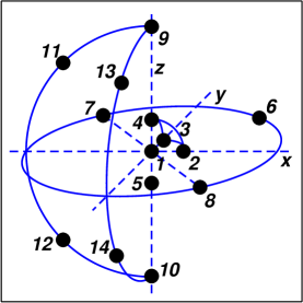
Figure 5: Positions of 14 electrons for the proof that triple exchanges connect the particles in the ${}^{15}S(1s2s2p^{3}3s3p^{3}3d^{5})$ state. Particles 2 to 5 lie on the spherical surface with the radius equal to the radial node of $\rho_{2s}(r)$ orbital. Particles 6 to 14 lie on the spherical surface with the radius equal to the radial node of $\rho_{2p}(r)$.

More difficult part of the proof is to show that one can exchange the particles between the subshells. We were able to prove analytically the exchange between $1s$ and $2s2p^{3}$ in our previous paper. For larger cases the analytic proof becomes very tedious and it is much more efficient to evaluate numerically the determinant along the following exchange paths. The particles are positioned as sketched in Fig.5 with the coordinates given by ${\bf r}_{1}=(0,0,0)$, ${\bf r}_{2}=(\eta_{a},0,0)$, ${\bf r}_{2}=(0,\eta_{a},0)$, ${\bf r}_{4,5}=(0,0,\pm\eta_{a})$, ${\bf r}_{6}=(\eta_{b}/\sqrt{2},\eta_{b}/\sqrt{2},0)$, ${\bf r}_{7,8}=(\pm\eta_{b}/\sqrt{2},\mp\eta_{b}/\sqrt{2},0)$, ${\bf r}_{9,10}=(0,0,\pm\eta_{b})$, ${\bf r}_{11,12}=(\eta_{b}/\sqrt{2},0,\pm\eta_{b}/\sqrt{2})$ and ${\bf r}_{13,14}=(0,\eta_{b}/\sqrt{2},\pm\eta_{b}/\sqrt{2})$. There exists enough of triple exchanges of neighbouring particles, along the sides of corresponding triangles, to connect all the particles into a single cluster. For example, the wave function values for exchanges $123\to 231$, $236\to 362$ (and other exchanges for illustration) are given in Fig. 6.

Figure 6: Wave function of the ${}^{15}S(1s2s2p^{3}3s3p^{3}3d^{5})$ state (arb. u.) along triple exchange paths parametrized by $t$. Particles are positioned as given in Fig. 5. The plotted exchanges: 1,2,3 (full line); 2,3,4 (dashed line); 2,3,6 (dotted line); 6,7,9 (dashed-dotted line); 9,11,13 (double dashed-dotted line). By symmetry, these non-crossing exchanges connect all the particles of this state.

This is enough to show that the three subshells are connected since many other exchanges are identical due to the symmetries in particle positions and the wave function $S$ symmetry. For the illustration in Fig. 6 we used the noninteracting radial orbitals. For HF orbitals one gets the same qualitative picture since the basic spatial properties of the noninteracting and HF orbitals are qualitatively the same (ie, ordering of radial nodes of $\rho_{nl}(r)$ orbitals, behaviour at nucleus, tails, etc). The proof uses only the fact that some of the radial nodes of the one-particle orbitals are ordered as in the non-interacting case so it can be extended to HF wave functions as well.

One can expand the proof to larger systems, such as for the state with occupied fourth main subshell $4s4p^{3}4d^{5}4f^{7}$ and beyond. The factorization is similar: the particles in the fourth subshell are positioned on the spherical surface with the radius equal to the radial node of $\rho_{4d}(r)$ orbital. Somewhat long but straightforward algebraic rearrangements show that the Slater determinant of the $30\times 30$ matrix can be reduced to product of subdeterminants corresponding to the subshells. For the purpose of this paper we do not deem necessary to go through the explicit proof.

VI VI. Interacting spin-unpolarized fermions.

It is straightforward to understand the fermion nodes of noninteracting spin-unpolarized or partially polarized systems with more than one-electron in each spin-channel. The wave function is a product of spin-up and -down Slater determinants and the number of nodal cells is the product of the number of cells in each subspace. (As mentioned before, we assume that the Hamiltonian, even with interactions considered below, does not include terms with spin so that particles can be assigned to the spin subspaces.) For the ground states with two nodal cells in each subspace we get $2\times 2=4$ nodal cells. This is the nodal structure of a single configuration Hartree-Fock wave function and as such has been used in many fixed-node QMC calculations. However, analyses of small interacting systems revealed that this is not correct and interactions do change the nodal topologies and the number of nodal cells. For the first time this has been demonstrated for the Be atom dariobe and then also for a few other atoms and small molecules cmt28 ; bajdichpfaffians .

In the previous paper mitasshort we have outlined a proof showing the two nodal domains property for $2D$ harmonic fermions in a closed-shell singlet state for arbitrary size. The most interesting feature of the proof was that the result was very robust in the sense that almost any arbitrary weak interaction would induce the change in the topology of the nodal surfaces.

We refresh some of the key notions and arguments here. Let us assume a spin-unpolarized system in its closed-shell singlet ground state of $2N$ particles. Consider a simultaneous exchange of an odd number of spin-up pair(s) and an odd number of spin-down pair(s). For noninteracting wave functions such simultaneous pair exchanges imply that the node will be crossed once or multiple times. This must be the case whenever the spin-up and -down subspaces are independent of each other, such as in the mean-field and HF wave functions. However, if there exists a point $R_{f}$ such that during the simultaneous spin-up and -down pair exchanges the inequality $|\Psi|>0$ holds along the whole path, then the wave function has only two nodal cells.

Using this property we can now demonstrate the two nodal cell for several types of systems. Under rather general conditions, we will show that the correlation included in the Bardeen-Cooper-Schrieffer (BCS) pairing wave function sorella ; carlson given by

$$\Psi_{BCS}(1,...,2N)={\rm det}[\Phi(i,j)]$$ (29)

smoothes out the noninteracting four nodal cells into the minimal two. Here $\Phi(i,j)=\Phi(j,i)$ is a singlet pair orbital for $i\negthinspace\negthinspace\uparrow$ and $j\negthinspace\negthinspace\downarrow$ fermions and we decompose it into noninteracting and correlated components $\Phi(i,j)=\Phi_{0}(i,j)+\Phi_{corr}(i,j)$. Using one-particle orbitals we can write $\Phi_{0}(i,j)=\sum_{\alpha}\negthinspace\phi_{\alpha}(i)\phi_{\alpha}(j)$ where the sum is over HF (or noninteracting) orbitals while $\Phi_{corr}(i,j)=\sum_{\alpha\beta}c_{\alpha\beta}\phi_{\alpha}(i)\phi_{\beta}(j)$ where $\{c_{\alpha\beta}=c_{\beta\alpha}\}$ are variational parameters and the sum is over unoccupied or virtual (”correlating”) orbitals. The BCS wave function was originally introduced for conventional superconductors, however, it proved to be very successful also in describing the correlation effects in electronic structure problems sorella ; bajdichpfaffians .

VI.1 VI.a. $3D$ harmonic spin-unpolarized fermions with interactions.

For the $3D$ harmonic oscillator one can show that the interactions lead to the minimal number of nodal cells in a rather simple and elegant way. First let us consider a small system which is easy to analyze. We illustrate the idea on $2N=8$ particles in the singlet ground state with the particle positions given in Fig. 7. The corresponding closed-shell singlet ground state for the $3D$ harmonic oscillator is ${}^{1}S(1s^{2}2p^{6})$. (Note that for the harmonic potential the $2p$ state is below the $2s$ state, unlike for the Coulomb potential.) For simplicity, we drop the gaussian prefactors since they do not affect the nodes and the pairing functions can be then written as follows

$$\Phi_{0}(i,j)=1+3{\bf r}_{i}\cdot{\bf r}_{j}$$ (30)

and

$$\Phi_{corr}(i,j)=\gamma[3({\bf r}_{i}\cdot{\bf r}_{j})^{2}-r_{i}^{2}r_{j}^{2}]$$ (31)

where the noninteracting part is constructed from the occupied $1s,2p$ orbitals while for the correlating part the unoccupied $3d$ subshell orbitals were used. The constant $\gamma$ is a variational parameter. Clearly, both the pair orbitals and the wave function are spherically symmetric. Assuming the positions as given in the Fig. 7, which are of high symmetry and therefore simplify the evaluation of the wave function, we get

$$\Psi(1,...,8)=4\gamma\cos\varphi[1-(3+\gamma)\cos^{2}\varphi]/3$$ (32)

where $r_{1}=r_{5}=0$, $\;r_{i}=1,i=2,3,4,6,7,8$ and $\cos\varphi={\bf r}_{4}\cdot{\bf r_{8}}$.

Figure 7: Positions of $2N=8$ fermions of the $3D$ harmonic well system. Fermions 1 to 4 have spins up, while 5 to 8 have spins down. Fermions 1 and 5 are at the origin while the rest of the particles lie on the surface of the sphere with $r=1$. Note that rotation of the system by $\pi$ around the $z-$axis exchanges particles $3,4$ and $7,8$. See the text for details.

For $\gamma=0$ the wave function vanishes since the particles in both spin subspaces lie on the noninteracting node (ie, four particles on the same plane). The key point is that for $\gamma\neq 0$ and $\varphi\neq\pi/2$ the wave function does not vanish. Since the wave function is spherically symmetric we can rotate the particles around the $z-$axis by $\pi$. This transformation exchanges particles 3 and 4 in the spin-up channel and particles 7 and 8 in the spin-down channel. The wave function is rotationally invariant and nonvanishing what clearly implies that the BCS wave function has spin-up and -down subspaces interconnected since simultaneous exchanges in the spin-up and spin-down does not hit the node. On the other hand, it is easy to check that the rotation of the particles in one spin channel only causes a node-crossing since then $\cos\varphi$ vanishes either at $\pi/2$ or $3\pi/2$.

It is clear that our argument is correct whenever the strength of the interaction is small so that the BCS wave function is accurate enough. The variational parameter $\gamma$ is related to the interaction strength. This implies that the topological change from two to four nodal cells takes place for arbitrary small, but nonvanishing, interaction strength. The only assumptions were that the interaction will induce electron correlation and lead to a nonzero variational parameter $\gamma$ (or, in general, to a nonvanishing correlation component) and that the wave function is spherically symmetric. Our analytic argument therefore shows that for weak interactions the nodal cell ”degeneracy” is lifted and the multiple cells are smoothed to the minimal number of two.

It is important to note that one can find different pictures in other circumstances. For example, for strong or nonlocal interactions, imposed additional symmetries or large degeneracies, the nodal changes can be different and the resulting nodal topology might exhibit more than the two nodal cells; this aspect is further discussed in the conclusion section and require more investigation.

Coming back to our example of harmonic fermions with interactions, using similar arguments the two nodal cells can be demonstrated for an arbitrary size closed-shell ground state. Consider $2N$ particles in a singlet closed-shell ground state. The closed-shell states can be labeled by $M$ which represents the ”Fermi momentum” for the harmonic oscillator and $N=(M+1)(M+2)(M+3)/6$. Let us decompose $N$ into the maximum odd number of pairs $N_{P}$ and the rest. Therefore we write $N=2N_{P}+J$ where $N_{P}$ is an odd integer while $J$ has one of the values $J=0,1,2,3$, so that we can also define $J=N\,{\it mod}\,4$. For example, in the previous example with $2N=8$ particles we have $N_{P}=1$ and $J=2$. First, we place $J$ particles from each spin channel on the $z$-axis in distinct positions. Next, we form $N_{P}$ pairs in each spin subspace so that, say, the pair $i\negthinspace\uparrow,(i+1)\negthinspace\uparrow$ is positioned as given by $(r_{i},\vartheta_{i},\varphi_{i})=(r_{k},\vartheta_{k},\varphi_{k})$, $\,(r_{i+1},\vartheta_{i+1},\varphi_{i+1})=(r_{k},\vartheta_{k},\varphi_{k}+\pi)$, where $r,\vartheta,\varphi$ are the spherical coordinates. Here $k=1,...,N_{P}$ labels the pairs in the spin-up channel; the spin-down particles are placed similarly and labeled by the pair index $l=N_{p}+1,...,2N_{P}$. In this configuration the particles lie on the noninteracting node since

$${\rm det}\left[\Phi_{0}(i,j)\right]={\rm det}\left[\sum_{n+m\leq M}\phi_{nm}(i)\phi_{nm}(j)\right]=$$

$$={\rm det}\left[\phi_{nm}(i)\right]{\rm det}\left[\phi_{nm}(j)\right]=\Psi_{HF}^{\uparrow}\Psi_{HF}^{\downarrow}$$ (33)

The rotation of the system by $\pi$ causes node-crossings in both spin channels so that both spin-up and -down Slater determinants must vanish due to the rotational invariance. Now, if all the $N_{P}$ pair distances and angles $r_{k},\varphi_{k},\vartheta_{k},r_{l},\vartheta_{l},\varphi_{l}$ are distinct, then each of the matrices $\left[\phi_{nm}(i)\right],\left[\phi_{nm}(j)\right]$ has exactly one linearly dependent row, ie, both have ranks $N_{P}-1$. This can be verified directly for small values of $M$ and then using induction for any $M$. Consequently, the matrix $\left[\Phi_{0}(i,j)\right]$ has linear dependence in one row and one column, ie, it has the rank of $N_{P}-1$ as well. In general, adding virtual states through $\Phi_{corr}(i,j)$ provides independent rows/columns which eliminate the linear dependency so that ${\rm det}\left[\Phi_{0}(i,j)+\Phi_{corr}(i,j)\right]$ is nonzero. Let us now assume that the interactions do not break the rotation invariance. Since at this point the wave function does not vanish and is rotationally invariant, it does not vanish for the whole exchange path implying that the correlated BCS wave function has only two nodal cells regardless of the size $2N$.

Clearly, the assumption of the rotational invariance for the interacting case might be too restrictive since the interactions could possibly break the spherical symmetry. To demonstrate the two nodal cells in such a case one would need to show that the wave function does not vanish for the complete exchange path.

VI.2 VI.b. $2D$ harmonic spin-unpolarized fermions with interactions for $N=2N_{P}+J$ when $J=2,3$.

In our previous paper we have demonstrated the two nodal cells for the ground states with the number of particles $2N$ where $N=2N_{P}+J$ and $J=0,1$. (We use the same notation as in $3D$ where $N_{P}$ is the maximum odd number of pairs and $J=0,1,2$ or 3). Note that the states with $J=0$ or 1 exist at any size. Here we would like to present an alternative and a little bit longer proof which covers $J=0,1$ but also remaining cases when $J=2,3$, eg, for $N=21=2\times 9+3,\;$ $N=28=2\times 13+2$, etc. In $3D$, the rotation axis can accommodate multiple particles so that one can always form an odd number of pairs for the exchanges. In $2D$, the symmetry point (origin) can accommodate only one particle from each spin subspace therefore the proof has to be modified. For this purpose we outline a factorization which is different from the previous paper mitasshort . Let us remind that for $2D$ harmonic oscillator the closed-shell states and the system size are labeled by $M=1,2,...$ where $n+m\leq M$ with the number of fermions in one spin channel given by $N=(M+1)(M+2)/2$. We express the one-particle states as polynomials in $r^{2}$ and $(re^{i\varphi})^{m}$ where $r,\varphi$ are the cylindric coordinates (we again omit the gaussian factors which are irrelevant for the nodes). Note that for a given $M$ the quantum number $m$ increases or decreases by 2 unlike in $3D$. Therefore for $M=2$ we have states $re^{\pm i\varphi}$, for $M=3$ the additional states are $(r^{2}-1),r^{2}e^{i\pm 2\varphi}$, etc. We first write down the wave functions for three- and six-particle spin-polarized systems with positions given in Fig. 8.

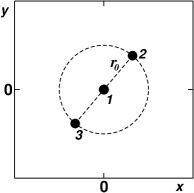
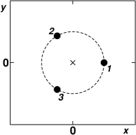
(a)		(b)
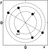
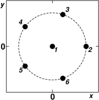
(c)		(d)

Figure 8: Alternative positions of three and six spin-polarized fermions for the $2D$ harmonic potential. (a) Three particles positioned on the noninteracting node. (b) Three particles in positions with a nonvanishing wave function. (c) Six particles positioned on the noninteracting node. (d) Six particles in positions with a nonvanishing wave function. See the text for details.

The three particle wave function is given by ${\rm det}\{1,re^{\pm i\varphi}\}$

$$\Psi_{2D}(1,2,3)=\mu_{0}r_{0}^{2}\prod_{1(2)\leq j<k\leq 3}\sin(\varphi_{jk}/2)$$ (34)

where $\mu_{0}$ is a constant. The product lower bound is 2 if the positions of the particles are as in Fig. 8a, while it is 1 if the positions are as in Fig. 8b. Note that in the case of configuration in Fig. 8a rotation by $\pi$ flips the wave function sign so that the wave function vanishes while for the configuration in Fig. 8b it does not. For six particles in the positions outlined in Fig. 8d the wave function is clearly nonvanishing since we can write

$$\Psi_{2D}(1,...,6)=\mu_{0}(r_{2}^{2}-r_{1}^{2})r_{2}^{6}\prod_{j<k}^{6}\sin(\varphi_{jk}/2)$$ (35)

where $\mu_{0}$ is some constant (in Fig. 8d we have $r_{1}=0$). Alternatively, the six particles can be positioned in pairs as sketched in Fig. 8c where the particles are positioned on the HF node so that the noninteracting wave function vanishes.

For the sake of completeness we provide the expression for the wave function for a general system with size $M$

$$\Psi_{2D}(1,...,N)=$$

$$=\mu(r_{1},...,r_{\tilde{M}})\prod_{k=1}^{\tilde{M}}\left[\Psi_{1D}(I_{k})\prod_{1\leq j<k}(r^{2}_{k}-r^{2}_{j})^{n_{j}}\right]$$ (36)

where $\tilde{M}={\rm int}[(M+1)/2]$ is the integer part of $(M+1)/2$. The particles with indices in the subset $I_{k}$ lie on a circle with the radius $r_{k}$ and $n_{k}=2(M+1-2k)+1$. The prefactor is again a nonnegative function of $r_{j}$ which has no impact on the nodes and is constant for rotations. From the last equation we see that in cases when $M$ is even, eg, $M=6,N=21$, we end up with factorization of the type $11\times 7\times 3$ particles while for $M$ odd, eg, $M=7,N=28$, we get $13\times 9\times 5\times 1$. That means that the last three particles ($M$ even) or the last six particles ($M$ odd) can be always arranged into possibilities as sketched in Fig 8a-d. It is now clear that we can prove that the spin-up and -down configuration space are interconnected for the cases when $J=2,3$ as specified above. Using the alternative configurations for three and six particles we can arrange the systems into such positions that the rotation by $\pi$ exchanges odd number of pairs in both spin channels. For example, if $N$ is odd and $(N-1)/2$ is even we position three particles on a triangle as given in Fig. 8b. That takes out one pair from the $(N-1)/2$ exchanges and the proof then follows using the arguments for $3D$ harmonic fermions. Similarly, if $N$ is even and $N/2$ is also even, we position one particle of each spin at the origin and five from each spin channel on a circle. This eliminates three pairs from $N/2$ and again we end up with remaining number of pairs being odd so that the rest of the proof follows similarly to the $3D$ case.

VI.3 VI.c. Spin unpolarized interacting $2D$ and $3D$ homogeneous electron gas.

Let us now prove the two nodal cells for the spin-unpolarized closed shells for $d>1$ homogeneous gas with interactions. We use the relevant definitions introduced previously for the spin-polarized periodic fermion gas (section III.a.). We assume a $2D$ system of $2N$ particles in the spin singlet ground state where the one-particle states occupy the Bloch states within the Fermi disk with the radius $k_{F}$. Let us first consider $2N=10$ particle case and we position the particles as in Fig. 9. The wave function is translationally invariant therefore the action of $T^{y}_{\pi}$ leaves the wave function unchanged. Assuming first that there is no interaction, we see that the translation exchanges the particles $1,2$ but due to the invariance the wave function value does not change: that is possible only if the particles are sitting on the node. This also agrees with expressions for the wave functions derived before (see Eq. 7.) Consider now that we switch-on interactions and describe the particles by the BCS wave function as given above. The pairing orbital for the noninteracting gas is given by

$$\Phi_{0}(i,j)=\sum_{|{\bf k}|\leq k_{F}}\phi_{\bf k}(i)\phi_{\bf-k}(j)=1+2[\cos(x_{ij})+\cos(y_{ij})]$$ (37)

where we used the occupied orbitals $\{1,e^{\pm ix},e^{\pm iy}\}$. The correlated part is given by

$$\Phi_{corr}(i,j)=\gamma\sum_{|{\bf k}|>k_{F}}\phi_{\bf k}(i)\phi_{\bf-k}(j)=$$

$$\gamma[\cos(x_{ij})\cos(y_{ij})+\cos(2x_{ij})+\cos(2y_{ij})]$$ (38)

where $\Phi_{corr}(i,j)$ includes the next two unoccupied stars of states with $k=\sqrt{2},2$ and $\gamma$ is a variational parameter.

Figure 9: Positions of five spin-up electrons from an interacting ten-fermion system in the $2D$ periodic box $(-\pi,\pi)^{2}$. For clarity, the five down-spin particles are not shown. The spin-down particles are positioned in the same pattern on two lines $x=const$.

Unlike for the noninteracting wave function (ie, $\gamma=0$) the BCS correlated wave function does not vanish and this is indeed the case due to the arguments presented above. The Slater matrix of uncorrelated wave function has linear dependency while for the correlated case there always exists a configuration of lines with nonvanishing wave function. This is due to the elimination of the linear dependency through addition of virtual orbitals, as explained for the $3D$ harmonic oscillator. Note that as soon as the wave function is translationally invariant the wave function does not vanish for the whole translation path, implying that the spin-up and -down nodal domains are interconnected and the wave function has only two nodal cells. It is straightforward to extend the proof to arbitrary size closed-shell system. The configuration of particles can be given as follows: an odd number of pairs (eg, one) in each spin channel is positioned in a similar way as in 9 so that the translation by $\pi$ exchanges the particles in the pair. For example, for a spin-up pair $i,i+1$ we specify the coordinates as $y_{i}=-y_{i+1}=\pi/2$ and $x_{i}=x_{i+1}=\xi_{0}$ where $\xi_{0}$ is distinct from $x$ coordinates of the rest of particles with the same spin. The rest of the particles is positioned in such a way so that the $T_{\pi}^{x}$ brings them into a symmetric position regarding the reflection around axis $y$. The wave function is translationally invariant and therefore uncorrelated wave function vanishes while for BCS case it is, in general, nonzero. The two nodal cells property then follows using the same general arguments as in the previous cases.

The correlated wave function has another important property namely that one can wind around the periodic box a singlet pair of particles (ie, spin-up and spin-down pair) without hitting the node. Indeed, this is implied by the fact that there are only two nodal cells: once this is the case one can then always find such a path that the pair of particles can wind around the box without node-crossing. For example, for the ten-particle example above we can wind spin-up and -down particle pair around along $y=\zeta_{0}$ without hitting the node. We plot the wave function for two types of particle positions: first, the spin-down particles are at identical positions as the spin-down ones, ie, ${\bf r}_{6}={\bf r}_{1}$, ${\bf r}_{7}={\bf r}_{2}$, etc (Fig. 10a); second, the particles in spin-up and -down channel were offset by small displacement ${\bf r}_{i+5}={\bf r}_{i}+0.2,$ $i=1,...,5$, see Fig. 10b. Consider now the simultaneous translation $T_{2\pi}^{y}$ of the particles 1 and 6. This translation winds the pair around the box and the wave function values for the paths are plotted in Fig. 10a,b. The value of the displacement between the particle positions neither the repositioning of the particles around the box is not crucial and there exists a significant size subspace of particle positions for which the winding of the pair is possible. We have chosen just two simple examples as qualitative illustrations.

Note that the wave function enables to wind also a single particle without the node crossing. However, single particle winding is possible both for correlated and uncorrelated wave functions since, say, the spin-up HF part has two nodal domains and correlated wave function only smoothes out the HF nodes. Therefore this property is not affected by the correlation in any significant manner.

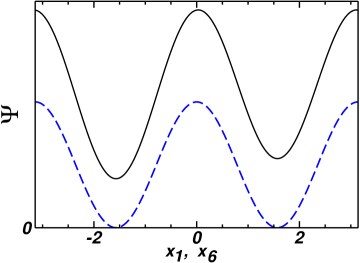
(a)

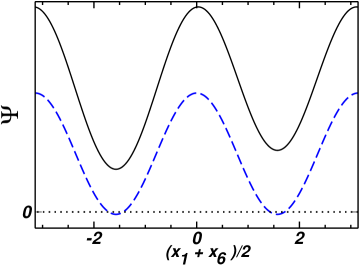
(b)

Figure 10: Winding the particles 1 (spin-up) and 6 (spin-down) around the $2D$ box along the line $y=\zeta_{0}$. The dashed line is the Hartree-Fock wave function (arb.u.) while the full line is the correlated BCS wave function. a) Particles 1 and 6, 2 and 7, etc, share the same position. The uncorrelated wave function touches the node quadratically since the spin-up and -down determinants are identical. b) The positions of particles in spin-down channel are offset by 0.2 from the positions in the particle spin-up channel. The uncorrelated wave function crosses the node multiple times since the spin-up and -down determinants are different.

The effect that singlet pair of particles can pass through nodal openings between the spin-up and -down subspaces have been demonstrated for small number of particles before, for example, in our paper on employing pfaffian pairing functions for electronic structure problems bajdichpfaffians . The case here illustrates that this property stems from interconnected spin-up and -down subspaces and therefore applies to similar two nodal cell wave functions, in general.

It is well known that a Fermi liquid, such as the homogeneous electron gas, becomes unstable to a weak attractive interaction, develops Cooper pair instability and opens the superconductivity gap supercond . This effect is captured by the BCS wave function which we used in the proof above. Cooper pairs can therefore wind around the box without hitting the node although this effect is not exclusive to Cooper pairs only. In fact, the connectedness of spin-up and -down subspaces is a rather generic property in the sense that it appears also in systems which are not necessarily superconducting, ie, in Fermi liquids with repulsive interactions. Since superconductivity is characterized by macroscopic phase coherence and a number of other properties, which might or might not be related to the nodal topologies, on the basis of the analysis of the BCS wave function above one expects that the nodal opening necessarily appears in the superconducting state, however, for the superconductivity to occur this condition is not sufficient. In addition, here we assume only the simplest $s-$wave pairing; for the $p-$wave or higher angular momentum pairing the situation is less clear and needs to be further investigated.

VII VII. Nodes of fermionic density matrices.

In this part we generalize the ideas presented in preceding section to temperature dependent density matrices davidnode . Consider first a system of spin-polarized fermions. The temperature/imaginary time density matrix is given by

$$\varrho(R^{\prime},R,\beta)=\sum_{n}e^{-\beta E_{n}}\Psi^{*}_{n}(R^{\prime})\Psi_{n}(R)$$ (39)

where $\beta$ is the inverse temperature and the sum is over the complete system of eigenstates of a given Hamiltonian $H$. It is clear that the density matrix is antisymmetric in particle exchanges in the same manner as the wave function $\Psi(R)$ or $\Psi(R^{\prime})$. Therefore the notion of fermion nodes can be generalized also to density matrix in $(2dN+1)$ dimensions since there is an explicit dependence on $\beta$ as well. As pointed out elsewhere davidnode , for fixed $R^{\prime}$ and $\beta$ one can study the nodes and nodal cells in the $dN$ dimensional $R-$subspace. Similarly to the wave function, the node then becomes $(dN-1)$-dimensional manifold with the generalization that it is dependent on $R^{\prime}$ and $\beta$. For the fixed $R^{\prime}$ and $\beta$ the tiling property holds in the same manner as for the wave functions. The key additional feature of the density matrix is that once there are only two nodal cells at some initial $\beta_{0}$ than this property holds for any $\beta>\beta_{0}$ davidnode . This is not difficult to understand since the density matrix fulfills the following linear equation

$$-{\partial\varrho(R,R^{\prime},\beta)\over\partial\beta}=H\varrho(R,R^{\prime},\beta)$$ (40)

with an initial condition

$$\varrho(R,R^{\prime},0)={\cal A}\delta(R-R^{\prime})={\det}[\delta({\bf r}_{i}-{\bf r^{\prime}}_{j})]$$ (41)

where ${\cal A}$ is the antisymmetrizing operator.

We now understand that for almost any Hamiltonian with interactions the density matrix will have only two nodal cells for sufficiently large $\beta$ (ie, at low temperatures). This is due to the fact that at sufficiently low temperature the ground state becomes dominant (Eq. 39). The key point now is to show that this is the case also for high temperatures. The free particle density matrix is given by

$$\varrho(R,R^{\prime},\beta)=(2\pi\beta)^{-dN/2}{\rm det}\left[\exp(-|{\bf r}_{i}-{\bf r^{\prime}}_{j}|^{2}/2\beta)\right]$$ (42)

where we assume atomic units with $\hbar^{2}/m=1$. (For other than free boundary conditions, such as for the periodic ones, the expression has to be modified accordingly.) Note that this density matrix is universal since at sufficiently high temperatures the interactions become irrelevant.

There are several ways how to prove that the high-temperature density matrix has only two nodal cells. For very small $\beta$ one can use the induction as follows. Assume that $N$ particles are described by the density matrix given by Eq. 42 and the particles are connected by triple exchanges for a fixed $R^{\prime},\beta$. We add an additional particle with the label $N+1$ to the system which occupies a certain region of the configuration (free) space. The particle $N+1$ is positioned at the border of the occupied region and let us assume that the particles with labels $N-1$ and $N$ are its closest neighbours. Let us move the three particles $N-1,N,N+1$ away from the rest without crossing the node (what can be always done by appropriate positioning). Since for small $\beta$ the overlaps of gaussians become small, one can factorize the determinant into a product of the three particles $N-1,N,N+1$ determinant and the determinant for the rest. For the three particles the density matrix has only two nodal cells as one can show easily davidnode and therefore the additional particle is connected. This applies to both $R$ and $R^{\prime}$ subspaces since they must have identical properties. (In what follows we will show that, in fact, at high temperatures the primed and unprimed spaces are connected as well.)

There is also an alternative proof which is interesting also on its own since it provides a different view on the density matrices. Note that the functional form of the free particle density matrix has a unique property. Comparing the Eq. 42 with the BCS wave function (Eq. 29) we see that the high-temperature density matrix can be identified with a BCS wave function if we properly define an underlying effective model. Instead of our original system of $N$ spin-polarized fermions, let as consider a model system with $2N$ particles so that the configurations $R$ and $R^{\prime}$ denote positions of these different sets of particles, which we will call for simplicity unprimed and primed particles. Let us then define a new Hamiltonian ${\tilde{H}}(R,R^{\prime})$ with an effective quadratic interaction between the unprimed and primed particles as given by

$${\tilde{H}}(R,R^{\prime})=T+T^{\prime}+V_{0}\beta^{-1}\sum_{i,j}|{\bf r}_{i}-{\bf r^{\prime}}_{j}|^{2}$$ (43)

where $T$ and $T^{\prime}$ denote kinetic energy operators for the corresponding sets of particles and $V_{0}$ is a constant with appropriate dimensions. Note that particles within the given set, say, unprimed, are antisymmetric but otherwise do not interact with each other. The interaction appears only between the primed and unprimed degrees of freedom as given by the Hamiltonian $\tilde{H}(R,R^{\prime})$. For $\beta\to 0$ the exact wave function for this system is a BCS wave function $\Psi(R,R^{\prime})={\rm det}[\phi({\bf r}_{i},{\bf r^{\prime}}_{j})]$ where the indices $i$ and $j$ label unprimed and primed particles, respectively. The pairing function $\phi({\bf r}_{i},{\bf r^{\prime}}_{j})$ is obviously the gaussian given above. It is not too difficult to demonstrate that this wave function (and the density matrix) has only two nodal cells. For example, we can expand the gaussian into plane waves

$$\exp(-|{\bf r}_{i}-{\bf r^{\prime}}_{j}|^{2}/2\beta)=\sum_{\bf k}c_{\bf k}e^{i{\bf k}\cdot({\bf r}_{i}-{\bf r^{\prime}}_{j})}$$ (44)

where $\{c_{\bf k}\}$ are expansion coefficients. The sum is over states within the Fermi sphere of a periodic box which accommodates $2N$ particles for a given density. Let us specify that $N$ is large and $\beta$ is such that the system can be considered classical so that the actual interaction in the original Hamiltonian $H$ is irrelevant. Then the density matrix corresponds to the Hartree-Fock product

$${\rm det}[e^{i{\bf k}_{i}\cdot{\bf r}_{j}}]{\rm det}[e^{-i{\bf k}_{i}\cdot{\bf r^{\prime}}_{j}}]$$ (45)

However, we have already proved that such system has only two nodal cells. In addition, if the sum includes also ”excited states” (ie, beyond the Fermi sphere) due to the primed-unprimed interactions, we find that the unprimed and primed nodal cells are interconnected. Therefore at classical temperature $\beta_{0}$ the density matrix has only two nodal cells and then the same is true for arbitrary $\beta>\beta_{0}$. This primed-unprimed interconnection becomes less pronounced and ceases to exist at $\beta\to\infty$ since then the density matrix is proportional to the ”noninteracting” product $\Psi_{0}(R)\Psi_{0}(R^{\prime})$ where $\Psi_{0}$ is the ground state for the original physical system of $N$ fermions described by $H$. This proof is therefore based on an interesting duality between the $N$ spin-polarized fermions at classical temperatures and the model system with $2N$ particles with a temperature-dependent, harmonic interaction between the unprimed and primed subspace particles.

Possibly, there might be also a third way how to prove the minimal number of nodal cells for the high-temperature density matrix through diagonalization of the quadratic Hamiltonian $\tilde{H}$ (we have not investigated this possibility). The fact that also the density matrices have two nodal cells is important for the path integral Monte Carlo methods which for fermions often employ the fixed-node approximation adapted for the path integrals davidhe .

VIII VIII. Discussion and conclusions.

Inspired by previous conjectures and numerical studies jbanderson ; davidnode ; lesternode ; sorella ; foulkes ; dariobe ; bajdichnode the presented analysis and proofs generalize and clarify the properties of ground states fermion nodes. We have employed symmetries, wave function factorizations and triple exchanges to prove that for $d>1$ the closed-shell ground states have two nodal cells for arbitrary number of particles in several paradigmatic models. In this paper the proofs were carried for closed shells, mainly to avoid additional complications from degeneracies and some of these aspects will be addressed in subsequent papers.

It is perhaps more interesting to discuss viable possibilities when the ground state wave functions might have more than two nodal cells. Clearly, it is easy to generate more nodal cells by imposing additional symmetry or boundary conditions. Another possibility comes from very strong interactions, for example, whenever the effect of interaction would become competitive with the kinetic energy increase from forming additional nodes it is possible that more than the minimal two nodal cells can form. One can also construct nonlocal interactions which would violate some of the properties mentioned here (eg, the tiling property), or reorder the states so that, for example, excited states could lie below the ground state, etc. Another candidate for unusual effects in the nodal structure are open-shell systems with large degeneracies and densities of states at the Fermi level. Some of these interesting issues will be subject of future studies.

In conclusion, we have presented a number of new results which reveal the structure of nodes and nodal cells of fermionic wave functions. Building upon ideas introduced in previous paper we were able to demonstrate the minimal number of two nodal cells in several spin-polarized models such as noninteracting fermions in a periodic box, in a box with zero boundary conditions, fermions on a spherical surface, etc. This enabled us to formulate a theorem which states that in $d>1$ the minimal two nodal cells are present for any Slater determinant with monomial matrix elements for any size which allows for a closed-shell nondegenerate ground state. We have shown that this property extends also to cases which cannot be described by the Slater matrix of monomials such as the noninteracting and HF atomic states up to the $3d$ shell. We have studied the effect of interactions on the noninteracting nodal cells of spin-unpolarized, closed-shell singlets. Our results show that, in general, the interactions smooth out the noninteracting multiple nodal cells into the minimal number of two. For interacting homogeneous electron gas we have demonstrated that the two nodal cells allow singlet pairs of particles to wind around the periodic box without crossing the node. Finally, we have shown that the temperature/imaginary time density matrix has very similar nodal structure and therefore the minimal two nodal cells property applies also to density matrices with important implications for path integral Monte Carlo simulations. We have demonstrated this by using an appropriate mapping of the density matrix onto the ground state of a model systems with twice as many particles interacting with temeperature-dependent harmonic potentials.

I am grateful to J. Kolorenč, M. Bajdich and L.K. Wagner for reading the manuscript, comments and discussions. I would like to acknowledge the support by NSF DMR-0102668, DMR-0121361 and EAR-0530110 grants.

References

- (1) D.M. Ceperley and M.H. Kalos, in Monte Carlo Methods in Statistical Physics, Ed. K. Binder, pp.145-194, Springer, Berlin, 1979; K.E. Schmidt and D. M. Ceperley, in Monte Carlo Methods in Statistical Physics II, pp.279-355, Ed. K. Binder, Springer, Berlin, 1984.
- (2) B.L. Hammond, W.A. Lester, Jr., and P.J. Reynolds, Monte Carlo Methods in ab initio quantum chemistry, World Scientific, Singapore, 1994.
- (3) M.W.C. Foulkes, L. Mitas, R.J. Needs and G. Rajagopal, Rev. Mod. Phys. 73, pp. 33-83 (2001).
- (4) J. B. Anderson, J. Chem. Phys. 65 4121 (1976); J. B. Anderson, Phys. Rev. A, 35, 3550 (1987).
- (5) D. M. Ceperley, J. Stat. Phys. 63, 1237 (1991).
- (6) W. A. Glauser, W. R. Brown, W. A. Lester, D. Bressanini, B. L. Hammond and M. L. Koszykowski, J. Chem. Phys. 97, 9200 (1992).
- (7) M. Casula and S. Sorella, J. Chem. Phys. 119, 6500 (2003)
- (8) W. M. C. Foulkes, Randolph Q. Hood and R. J. Needs, Phys. Rev. B 60, 4558 (1999).
- (9) D. Bressanini, D. M. Ceperley and P. Reynolds, in Recent Advances in Quantum Monte Carlo Methods, II Ed. W. A. Lester, S. M. Rothstein, and S. Tanaka, World Scientific, Singapore (2002).
- (10) D. Bressanini,and P. Reynolds, Phys. Rev. Lett. 95, 110201 (2005).
- (11) M. Bajdich, L. Mitas, G. Drobny, and L. K. Wagner, Phys. Rev. B 72, 075131 (2005)
- (12) L. Mitas, G. Drobny, M. Bajdich, L.K. Wagner, in Condensed Matter Theories, Vol.20, Eds. J.W. Clark, R.M. Panoff, and H. Li, Nova Science Publishers, New York, 2006; cond-mat/0409406.
- (13) M. Berger, A Panoramic View of Riemannian Geometry, Springer, Berlin, 2000, p.84.
- (14) A. N. Varchenko, Math. USSR Izvestiya, N.3, 35, 543 (1990)
- (15) C. K. Chui and L. M. Lai, in Nonlinear and Convex Analysis, Eds. B.L. Lin and S.Simons, pp. 23-35, Marcel Dekker, 1987.
- (16) M. Bajdich, G. Drobny, L.K. Wagner, and K. E. Schmidt, Phys. Rev. Lett. 96, 130201 (2006).
- (17) L. Mitas, submitted, cond-mat/0601485
- (18) J. Carlson, S.-Y. Chang, V. R. Pandharipande, and K. E. Schmidt, Phys. Rev. Lett. 91, 050401 (2003).
- (19) R. Shankar, Rev. Mod. Phys. 66, 000129 (1994); A. J. Leggett, Rev. Mod. Phys. 47, 331 (1975); H. Bruus and K. Flensberg, Many-Body Quantum Theory in Condensed Matter Physics, Oxford University Press, Oxford, 2004, p. 325.
- (20) D.M. Ceperley, Rev. Mod. Phys. 67, 279 (1995).