Onsager-Machlup theory for nonequilibrium steady states and fluctuation theorems

Abstract

A generalization of the Onsager-Machlup theory from equilibrium to nonequilibrium steady states and its connection with recent fluctuation theorems are discussed for a dragged particle restricted by a harmonic potential in a heat reservoir. Using a functional integral approach, the probability functional for a path is expressed in terms of a Lagrangian function from which an entropy production rate and dissipation functions are introduced, and nonequilibrium thermodynamic relations like the energy conservation law and the second law of thermodynamics are derived. Using this Lagrangian function we establish two nonequilibrium detailed balance relations, which not only lead to a fluctuation theorem for work but also to one related to energy loss by friction. In addition, we carried out the functional integrals for heat explicitly, leading to the extended fluctuation theorem for heat. We also present a simple argument for this extended fluctuation theorem in the long time limit.

I Introduction

Fluctuations play an important role in descriptions of nonequilibrium phenomena. A typical example is the fluctuation-dissipation theorem, which connects transport coefficients to fluctuations in terms of auto-correlation functions. This theorem can be traced back to Einstein’s relation E05 , Nyquist’s theorem J28 ; N28 , Onsager’s arguments for reciprocal relations O31a ; O31b ; C45 , etc., and it was established in linear response theory in nonequilibrium statistical mechanics near equilibrium G51 ; CW51 ; K57 . Another example of fluctuation theories is Onsager-Machlup’s fluctuation theory around equilibrium H52 ; OM53 ; MO53 . It is characterized by the usage of a functional integral technique for stochastic linear relaxation processes, and leads to a variational principle known as Onsager’s principle of minimum energy dissipation. Many efforts have been devoted to obtain a generalization, for example, to the cases of nonlinear dynamics H76 ; H77 ; Y71 ; HR81 ; R89 and nonequilibrium steady states BSG01 ; BSG02 ; G02 .

Recently, another approach to fluctuation theory leading to fluctuation theorems has drawn considerable attention in nonequilibrium statistical physics ECM93 ; ES94 ; GC95 . They are asymmetric relations for the distribution functions for work, heat, etc., and they may be satisfied even in far from equilibrium states or for non-macroscopic systems which are beyond conventional statistical thermodynamics. Originally they were proposed for deterministic chaotic dynamics, but they can also be justified for stochastic systems K98 ; LS99 ; C99 ; C00 . Moreover, laboratory experiments to check these fluctuation theorems have been made CL98 ; WSM02 ; CGH04 ; FM04 ; GC05 ; SST05 .

From our accumulated knowledge on fluctuations, it is meaningful to ask for relations among the different fluctuation theories. It is already known that the fluctuation-dissipation theorem, as well as Onsager’s reciprocal relations, can be derived from fluctuation theorems near equilibrium states ECM93 ; LS99 ; G96 . The heat fluctuation theorem can also be regarded as a refinement of the second law of thermodynamics.

The principal aims of this paper are twofold. First, we generalize Onsager and Machlup’s original fluctuation theory around equilibrium to fluctuations around nonequilibrium steady states using the functional integral approach. For this nonequilibrium steady state Onsager-Machlup theory we discuss the energy conservation law (i.e. the analogue of the first law of thermodynamics), the second law of thermodynamics, and Onsager’s principle of minimum energy dissipation. As the second aim of this paper, we discuss fluctuation theorems based on our generalized Onsager-Machlup theory. Since the systems we consider are in a nonequilibrium steady state, the equilibrium detailed balance condition is violated. We propose generalized forms of the detailed balance conditions for nonequilibrium steady states, which we call nonequilibrium detailed balance relations, and show that the fluctuation theorem for work can be derived from it. To demonstrate the efficacy of nonequilibrium detailed balance as an origin of fluctuation theorems, we also show another form of nonequilibrium detailed balance, which leads to another fluctuation theorem for energy loss by friction. We also show how a heat fluctuation theorem can be derived from our generalized Onsager-Machlup theory, by carrying out explicitly a functional integral and reducing its derivation to a previous one discussed in Refs. ZC03a ; ZC04 . In addition, we give a simple argument leading to the long-time ($t\rightarrow+\infty$) fluctuation theorem for heat, based on the independence between the work distribution and the energy-difference distribution.

In this paper, in order to make our arguments as concrete and simple as possible, we apply our theory to a specific nonequilibrium Brownian particle model described by a Langevin equation (cf. S98 ). It has been used to discuss fluctuation theorems MJ99 ; TTM02 ; ZC03a ; ZC03b ; ZC04 , and also to describe laboratory experiments for a Brownian particle captured in an optical trap which moves with a constant velocity through a fluid WSM02 ; TTM02 , as well as for an electric circuit consisting of a resistor and capacitor ZCC04 ; GC05 .

The outline of this paper is as follows. In Sec. II, we introduce our model and give some of its properties using a functional integral approach. In Sec. III, we discuss a generalization of Onsager-Machlup’s fluctuation theory to nonequilibrium steady states, and obtain the energy conservation law, the second law of thermodynamics, i.e. a nonequilibrium steady state thermodynamics, and Onsager’s principle of minimum energy dissipation for such states. In Sec. IV, we introduce the concept of nonequilibrium detailed balance, and obtain a fluctuation theorem for work from it. In Sec. V, we discuss another type of nonequilibrium detailed balance, which leads to a fluctuation theorem for energy loss by friction. In Sec. VI, we sketch a derivation of a fluctuation theorem for heat by carrying out a functional integral and reducing it to the previous derivation ZC03a ; ZC04 . In addition, we give a simple argument for the heat fluctuation theorem in the long time limit. In Sec. VII, we briefly discuss inertial effects on the fluctuation theorems, which lead to four new fluctuation theorems. In Sec. VIII, we summarize our results in this paper and discuss some consequences of them.

II Dragged Particle in a Heat Reservoir

The system considered in this paper is a particle dragged by a constant velocity $v$ in a fluid as a heat reservoir. The dynamics of this system is expressed as a Langevin equation noteIIa

$$m\frac{d^{2}x_{t}}{dt^{2}}=-\alpha\frac{dx_{t}}{dt}-\kappa\left(x_{t}-vt\right)+\zeta_{t}$$ (1)

for the particle position $x_{t}$ at time $t$ in the laboratory frame. Here, $m$ is the particle mass, and on the right-hand side of Eq. (1) the first term is the friction force with the friction constant $\alpha$, the second term is the harmonic potential force with the spring constant $\kappa$ to confine the particle, and the third term, due to the coupling to the heat reservoir, is a Gaussian-white noise $\zeta_{t}$, whose first two auto-correlations are given by

$$\langle\zeta_{t}\rangle = 0,$$ (2)

$$\langle\zeta_{t_{1}}\zeta_{t_{2}}\rangle = \frac{2\alpha}{\beta}\delta(t_{1}-t_{2})$$ (3)

with the inverse temperature $\beta$ of the reservoir and the notation $\langle\cdots\rangle$ for an initial ensemble average. The coefficient $2\alpha/\beta$ in Eq. (3) is determined by the fluctuation-dissipation theorem, so that in the case $v=0$ the stationary state distribution function for the dynamics (1) is expressed by a canonical distribution. A schematic illustration for this system is given in Fig. 1.

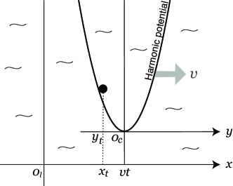
Figure 1: Schematic illustration for a particle trapped by a harmonic potential dragged with a constant velocity $v$ in a reservoir. Here, $x$ and $y$ ($0_{l}$ and $0_{c}$) are the axes (the origins) for the laboratory and comoving frame, respectively, in the direction of the motion of the particle. The particle is at the position $y_{t}$ ($x_{t}$) at time $t$ in the comoving (laboratory) frame, respectively, which are related by $y_{t}=x_{t}-vt$. After the relaxation time $\tau$, the system will reach a nonequilibrium steady state.

In this paper, except in Sec. VII, we consider the over-damped case in which we neglect the inertial term $md^{2}x_{t}/dt^{2}$, or assume simply an negligible small mass $m$. Under this over-damped assumption, the Langevin equation (1) can be written as

$$\frac{dx_{t}}{dt}=-\frac{1}{\tau}\left(x_{t}-vt\right)+\frac{1}{\alpha}\zeta_{t}$$ (4)

with the relaxation time $\tau$ given by $\tau\equiv\alpha/\kappa$.

Equation (4) is for the position $x_{t}$ in the laboratory frame. On the other hand, it is often convenient or simpler to discuss the nonequilibrium dynamics in the comoving frame TM04 ; ZC03b . The position $y_{t}$ in the comoving frame for the particle in our model is simply introduced as

$$y_{t}\equiv x_{t}-vt.$$ (5)

Using this position $y_{t}$, Eq. (4) can be rewritten as

$$\frac{dy_{t}}{dt}=-\frac{1}{\tau}y_{t}-v+\frac{1}{\alpha}\zeta_{t},$$ (6)

whose dynamics is invariant under the change $y_{t}\rightarrow-y_{t}$ and $v\rightarrow-v$, noting that the Gaussian-white noise property of $\zeta_{t}$ is not changed into $\zeta_{t}\rightarrow-\zeta_{t}$. Note that in the comoving Langevin equation (6) there is no explicit $t$-dependent term in the dynamical equation, while the laboratory Langevin equation (4) has a $t$-dependence through the term $vt$, meaning Eq. (6) to be a little simpler than Eq. (4). The constant term $-v$ in Eq. (6) expresses all effects of the nonequilibrium steady state in this model.

The system described by the Langevin equation (6), or equivalently Eq. (4), approaches a nonequilibrium steady state, because the particle will, for $t>\tau$, move steadily due to the external force that drags it through the fluid. This force is given by $-\kappa y_{t}$, so the work rate $\dot{\mathcal{W}}^{(v)}(y_{t})$ to keep the particle in a steady state is expressed as

$$\dot{\mathcal{W}}^{(v)}(y_{t})=-\kappa y_{t}v.$$ (7)

We note that since $\dot{\mathcal{W}}^{(0)}(y_{t})=0$ for $v=0$, i.e. for the equilibrium state considered by Onsager and Machlup, there is no work done, while in the nonequilibrium steady state for $v\neq 0$ work is done note2a .

We consider the transition probability ${F}\!(\begin{array}[]{c}\!\!\scriptstyle{y_{t}}\!\!\\ \!\!\scriptstyle{t}\!\!\end{array}|\begin{array}[]{c}\!\!\scriptstyle{y_{0}}\!\!\\ \!\!\scriptstyle{t_{0}}\!\!\end{array})$ of the particle from $y_{0}(\equiv y_{t_{0}})$ at time $t_{0}$ to $y_{t}$ at time $t$, which is introduced as a transition integral kernel for the probability distribution $f(y_{t},t)$ at the position $y_{t}$ at time $t$ as

$$f(y_{t},t)=\int dy_{0}\;{F}\!\left(\begin{array}[]{c}\!\!y_{t}\!\!\\ \!\!t\!\!\end{array}\right|\left.\begin{array}[]{c}\!\!y_{0}\!\!\\ \!\!t_{0}\!\!\end{array}\right)f(y_{0},t_{0})$$ (12)

with the initial distribution $f(y_{0},t_{0})$. We can use various analytical techniques, for example the Fokker-Planck equation, whose solution gives the probability distribution $f(y_{t},t)$ K92 ; R89 , to analyze the transition probability for the dynamics expressed by the Langevin equation (6). As one such technique, motivated by Ref. OM53 ; MO53 , we use in this paper the functional integral technique R89 . Using this technique, the transition probability is represented as

$${F}\!\left(\begin{array}[]{c}\!\!y_{t}\!\!\\ \!\!t\!\!\end{array}\right|\left.\begin{array}[]{c}\!\!y_{0}\!\!\\ \!\!t_{0}\!\!\end{array}\right)=\int_{y_{0}}^{y_{t}}\mathcal{D}y_{s}\;\exp\left[\int_{t_{0}}^{t}ds\;L^{(v)}\!\left(\dot{y}_{s},y_{s}\right)\right]$$ (17)

where $L^{(v)}\!\left(\dot{y}_{s},y_{s}\right)$ is the Lagrangian function for this stochastic process, defined by

$$L^{(v)}\!\left(\dot{y}_{s},y_{s}\right)\equiv-\frac{1}{4D}\left(\dot{y}_{s}+\frac{1}{\tau}y_{s}+v\right)^{2},$$ (18)

where $D$ is the diffusion constant given by the Einstein relation $D\equiv 1/(\alpha\beta)$. [We outline a derivation of Eq. (17) from Eq. (6) in Appendix A.] Here, the functional integral on the right-hand side of Eq. (17) is introduced as

$$\int_{y_{0}}^{y_{t}}\mathcal{D}y_{s}\;X_{t}(\{y_{s}\})$$

$$=\lim_{N\rightarrow+\infty}\left(\frac{1}{4\pi D\Delta t_{N}}\right)^{N/2}$$

$$\hskip 22.76228pt\times\int dy_{t_{N-1}}\int dy_{t_{N-2}}\cdots\int dy_{t_{1}}\;X_{t}(\{y_{s}\})$$

(19)

for any functional $X_{t}(\{y_{s}\})$, with $t_{n}\equiv t_{0}+n\Delta t_{N}$, $n=1,2,\cdots,N$, $\Delta t_{N}\equiv(t-t_{0})/N$, the initial time $t_{0}$, the final time $t_{N}=t$, the initial position $y_{0}$, and the final position $y_{t}$. Here, we use the symbol $\{y_{s}\}$ in $X_{t}(\{y_{s}\})$ to show that $X_{t}(\{y_{s}\})$ is a functional of $\{y_{s}\}$ with $s\in[t_{0},t]$. It is important to note that from the representation (17) of the transition probability ${F}\!(\begin{array}[]{c}\!\!\scriptstyle{y_{t}}\!\!\\ \!\!\scriptstyle{t}\!\!\end{array}|\begin{array}[]{c}\!\!\scriptstyle{y_{0}}\!\!\\ \!\!\scriptstyle{t_{0}}\!\!\end{array})$ the functional $\exp[\int_{t_{0}}^{t}ds\;L^{(v)}(\dot{y}_{s},y_{s})]$ can be regarded as the probability functional density of the path $\{y_{s}\}_{s\in[t_{0},t]}$.

For the Lagrangian function (18), the functional integral on the right-hand side of Eq. (17) can actually be carried out using Eq. (19), to obtain, by a simple generalization of the well-known equilibrium ($v=0$) case,

$${F}\!\left(\begin{array}[]{c}\!\!y_{t}\!\!\\ \!\!t\!\!\end{array}\right|\left.\begin{array}[]{c}\!\!y_{0}\!\!\\ \!\!t_{0}\!\!\end{array}\right) = \frac{1}{\sqrt{4\pi D\mathcal{T}_{t}}}$$

$$\times\exp\left\{-\frac{\left[y_{t}+v\tau-\left(y_{0}+v\tau\right)b_{t}\right]^{2}}{4D\mathcal{T}_{t}}\right\},$$

where $b_{t}$ and $\mathcal{T}_{t}$ are defined by $b_{t}\equiv\exp[-(t-t_{0})/\tau]$ and $\mathcal{T}_{t}\equiv(\tau/2)(1-b_{t}^{2})$ so that $\mathcal{T}_{t}=t-t_{0}+\mathcal{O}((t-t_{0})^{2})$ noteIIA . Equation (LABEL:TransProba2) is simply a well known form of the transition probability for the Smoluchowski process R89 . Inserting Eq. (LABEL:TransProba2) into Eq. (12), using the normalization condition $\int dy_{0}\;f(y_{0},t_{0})=1$, and taking the limit $t\rightarrow+\infty$, we can show that for an arbitrary initial distribution $f(y_{0},t_{0})$, the probability distribution $f(y_{t},t)$ approaches to a nonequilibrium steady state (ss) distribution:

$$f_{ss}(y_{t})\equiv\lim_{t\rightarrow+\infty}f(y_{t},t)=f_{eq}\left(y_{t}+v\tau\right)$$ (26)

in the long time limit. Here, $f_{eq}(y)$ is the equilibrium distribution function given by

$$f_{eq}(y)=\sqrt{\frac{\kappa\beta}{2\pi}}\exp\left[-\beta U(y)\right]$$ (27)

with the harmonic potential energy $U(y)\equiv\kappa y^{2}/2$. Equation (26) implies that the steady state distribution $f_{ss}(y)$ is simply given by the equilibrium canonical distribution $f_{eq}(y)$ by shifting the position $y$ to $y+v\tau$. [Note that there is no kinetic energy term in the canonical distribution (27) under the over-damped assumption.] Equation (26) implies that the average position of the particle is shifted from the bottom $y=0$ of the harmonic potential in the equilibrium state to the position $y=-v\tau$ in the nonequilibrium steady state.

The functional integral approach has already been used to describe relaxation processes to thermal equilibrium with fluctuations and averages by Onsager and Machlup OM53 ; MO53 . In the next section, we generalize their argument to non-equilibrium steady states for our model, and construct a nonequilibrium steady state thermodynamics. The results in Refs. OM53 ; MO53 can always be reproduced from our results in Sec. III by taking $v=0$, i.e. in the equilibrium case. In this generalization, we determine the work to sustain the nonequilibrium steady state in the Onsager-Machlup theory, and also give a direct connection between the entropy production rate in the Onsager-Machlup theory and the heat discussed in Ref. ZC03a ; ZC04 .

III Onsager-Machlup Theory for Nonequilibrium Steady states

In the generalized Onsager-Machlup theory, the Lagrangian $L^{(v)}\!\left(\dot{y}_{s},y_{s}\right)$ can be written in the form

$$L^{(v)}(\dot{y}_{s},y_{s})=-\frac{1}{2k_{B}}\left[\Phi^{(v)}(\dot{y}_{s})+\Psi(y_{s})-\dot{\mathcal{S}}^{(v)}(\dot{y}_{s},y_{s})\right]$$

(28)

where $k_{B}$ is the Boltzmann constant, and $\Phi^{(v)}(\dot{y}_{s})$, $\Psi(y_{s})$ and $\dot{\mathcal{S}}^{(v)}(\dot{y}_{s},y_{s})$ are defined by

$$\Phi^{(v)}(\dot{y}_{s}) \equiv \frac{\alpha}{2T}(\dot{y}_{s}+v)^{2},$$ (29)

$$\Psi(y_{s}) \equiv \frac{\alpha}{2T}\left(\frac{y_{s}}{\tau}\right)^{2},$$ (30)

$$\dot{\mathcal{S}}^{(v)}(\dot{y}_{s},y_{s}) \equiv -\frac{1}{T}\kappa y_{s}(\dot{y}_{s}+v),$$ (31)

respectively, with the temperature $T\equiv(k_{B}\beta)^{-1}$. These functions $\Phi^{(v)}(\dot{y}_{s})$ and $\Psi(y_{s})$ are called dissipation functions, while we call $\dot{\mathcal{S}}^{(v)}(\dot{y}_{s},y_{s})$ the entropy production rate. In the next subsections III.1 and III.2, we discuss the physical meaning of these quantities, and justify their names.

III.1 Heat and energy balance equations

Using the entropy production rate $\dot{\mathcal{S}}^{(v)}(\dot{y}_{s},y_{s})$, we introduce the heat $\mathcal{Q}^{(v)}_{t}(\{y_{s}\})$ produced by the system in the time-interval $[t_{0},t]$ as

$$\mathcal{Q}^{(v)}_{t}(\{y_{s}\})\equiv T\int_{t_{0}}^{t}ds\;\dot{\mathcal{S}}^{(v)}(\dot{y}_{s},y_{s}).$$ (32)

On the other hand, the work $\mathcal{W}_{t}^{(v)}(\{y_{s}\})$ done on the system to sustain it in a steady state is given by

$$\mathcal{W}_{t}^{(v)}(\{y_{s}\})\equiv\int_{t_{0}}^{t}ds\;\dot{\mathcal{W}}^{(v)}(y_{s}).$$ (33)

using the work rate (7). The heat (32) and the work (33) are related by

$$\mathcal{Q}^{(v)}_{t}(\{y_{s}\})=\mathcal{W}_{t}^{(v)}(\{y_{s}\})-\Delta\mathcal{U}(y_{t},y_{0})$$ (34)

with the internal (potential) energy difference

$$\Delta\mathcal{U}(y_{t},y_{0})\equiv U(y_{t})-U(y_{0})$$ (35)

at times $t$ and $t_{0}$. The relation (34) is nothing but the energy conservation law satisfied even by fluctuating quantities. It may be noted that Eq. (34) is used as a “definition” of heat in Ref. ZC03a ; ZC04 , while here it appears as a consequence of our nonequilibrium Onsager-Machlup theory. In other words, our generalization of the Onsager-Machlup theory gives a justification of the heat used in Ref. ZC03a ; ZC04 . For other attempts to justify the energy conservation law in stochastic processes using a Langevin equation or a master equation, see Refs. S98 ; C00 .

III.2 Dissipation functions and the entropy production

First, it follows from Eqs. (29) and (31) that

$$\Phi^{(-v)}(-\dot{y}_{s}) = \Phi^{(v)}(\dot{y}_{s}),$$ (36)

$$\dot{S}^{(-v)}(-\dot{y}_{s},y_{s}) = -\dot{S}^{(v)}(\dot{y}_{s},y_{s}),$$ (37)

implying that the dissipation function $\Phi^{(v)}(\dot{y}_{s})$ [as well as $\Psi(y_{s})$ by Eq. (30)] is invariant under the time-reversal changes $\dot{y}_{s}\rightarrow-\dot{y}_{s}$ and $v\rightarrow-v$, while the entropy production rate $\dot{S}^{(v)}(\dot{y}_{s},y_{s})$ is anti-symmetric under these changes. It is also obvious from Eqs. (29) and (30) that

$$\Phi^{(v)}(\dot{y}_{s}) \geq 0,$$ (38)

$$\Psi(y_{s}) \geq 0,$$ (39)

namely, that the dissipation functions are non-negative. One should also notice that by the definitions (29) and (30) the dissipation functions $\Phi^{(v)}(\dot{y}_{s})$ and $\Psi(y_{s})$ are proportional to the friction constant $\alpha$.

Second, from Eqs. (2) and (6), the ensemble average $\langle y_{s}\rangle$ of the particle position $y_{s}$ satisfies

$$\langle\dot{y}_{s}\rangle=-\frac{1}{\tau}\langle y_{s}\rangle-v,$$ (40)

with the time-derivative $\dot{y}_{s}\equiv dy_{s}/ds$ of $y_{s}$, leading to $\langle y_{s}\rangle=-v\tau+(\langle y_{0}\rangle+v\tau)\exp[-(s-t_{0})/\tau]$. Using this average position $\langle y_{s}\rangle$ and the average velocity $\langle\dot{y}_{s}\rangle$, it follows from Eqs. (29), (30) and (40) that

$$\Phi^{(v)}(\langle\dot{y}_{s}\rangle)=\Psi(\langle y_{s}\rangle).$$ (41)

Namely, the two dissipation functions $\Phi^{(v)}(\dot{y}_{s})$ and $\Psi(y_{s})$ have the same value for $\langle y_{s}\rangle$ and $\langle\dot{y}_{s}\rangle$, although $\Phi^{(v)}(\dot{y}_{s})$ is a function of $\dot{y}_{s}$ and $\Psi(y_{s})$ is a function of $y_{s}$. Moreover, from Eqs. (29), (31), (38), (40) and (41) we derive

$$\dot{S}^{(v)}(\langle\dot{y}_{s}\rangle,\langle y_{s}\rangle)=2\Phi^{(v)}(\langle\dot{y}_{s}\rangle)=2\Psi(\langle y_{s}\rangle)\geq 0,$$ (42)

namely, the function $2\Phi^{(v)}(\langle\dot{y}_{s}\rangle)$ [as well as $2\Psi(\langle y_{s}\rangle)$] gives the entropy production rate $\dot{S}^{(v)}(\langle\dot{y}_{s}\rangle,\langle y_{s}\rangle)$, justifying the name “dissipation function” for $\Phi^{(v)}(\dot{y}_{s})$ and $\Psi(y_{s})$. The inequality in (42) is the second law of thermodynamics in the Onsager-Machlup theory.

III.3 Onsager’s principle of minimum energy dissipation and the most probable path

Equation (40) for the average $\langle y_{s}\rangle$ of the particle position can be derived from the variational principle

$$\Phi^{(v)}(\dot{y}_{s})+\Psi(y_{s})-\dot{\mathcal{S}}^{(v)}(\dot{y}_{s},y_{s})=\mbox{minimum},$$ (43)

without using the Langevin equation (6). This can be proved by using that $\Phi^{(v)}(\dot{y}_{s})+\Psi(y_{s})-\dot{\mathcal{S}}^{(v)}(\dot{y}_{s},y_{s})=-2k_{B}L^{(v)}(\dot{y}_{s},y_{s})\geq 0$ and $L^{(v)}(\langle\dot{y}_{s}\rangle,\langle y_{s}\rangle)=0$, so that the left-hand side of Eq. (43) takes its minimum value for $y_{s}=\langle y_{s}\rangle$, i.e. for the average path, which is used in Eq. (42). Equation (43) is called the Onsager’s principle of minimum energy dissipation, and is proposed as a generalization of the maximal entropy principle for equilibrium thermodynamics OM53 ; MO53 ; TM57 ; O31a ; O31b ; H76 ; H77 .

Another result in the Onsager-Machlup theory as a variational principle is that we can justify a variational principle to extract the special path $\{y_{s}^{*}\}_{s\in[t_{0},t]}$, the so-called most probable path, which give the most significant contribution in the transition probability ${F}\!(\begin{array}[]{c}\!\!\scriptstyle{y_{t}}\!\!\\ \!\!\scriptstyle{t}\!\!\end{array}|\begin{array}[]{c}\!\!\scriptstyle{y_{0}}\!\!\\ \!\!\scriptstyle{t_{0}}\!\!\end{array})$. By the expression (17) for the transition probability ${F}\!(\begin{array}[]{c}\!\!\scriptstyle{y_{t}}\!\!\\ \!\!\scriptstyle{t}\!\!\end{array}|\begin{array}[]{c}\!\!\scriptstyle{y_{0}}\!\!\\ \!\!\scriptstyle{t_{0}}\!\!\end{array})$, the most probable path $\{y_{s}^{*}\}_{s\in[t_{0},t]}$ is determined by the maximal condition on $\int_{t_{0}}^{t}ds\;L^{(v)}\!\left(\dot{y}_{s},y_{s}\right)$, in other words, the path $\{y_{s}\}_{s\in[t_{0},t]}$ satisfying

$$\int_{t_{0}}^{t}ds\;\left[\Phi^{(v)}(\dot{y}_{s})+\Psi(y_{s})-\dot{\mathcal{S}}^{(v)}(\dot{y}_{s},y_{s})\right]=\mbox{minimum},$$

(44)

under fixed values of $y_{0}$ and $y_{t}$, noting the expression (28) for the Lagrangian function $L^{(v)}\!\left(\dot{y}_{s},y_{s}\right)$. The condition (44), or equivalently the maximal condition of $\int_{t_{0}}^{t}ds\;L^{(v)}\!\left(\dot{y}_{s},y_{s}\right)$ implies the variational principle $\delta\int_{t_{0}}^{t}ds\;L^{(v)}\!\left(\dot{y}_{s},y_{s}\right)=0$ for the path $\{y_{s}\}_{s\in[t_{0},t]}$, leading to the Euler-Lagrange equation LL69

$$\frac{d}{ds}\frac{\partial L^{(v)}(\dot{y}^{*}_{s},y^{*}_{s})}{\partial\dot{y}^{*}_{s}}-\frac{\partial L^{(v)}(\dot{y}^{*}_{s},y^{*}_{s})}{\partial y^{*}_{s}}=0$$ (45)

for the most probable path $\{y_{s}^{*}\}_{s\in[t_{0},t]}$. (The most probable path can also be analyzed by the Hamilton-Jacobi equation BSG01 ; BSG02 .) Inserting Eq. (18) into Eq. (45) we obtain

$$\frac{d^{2}y^{*}_{s}}{ds^{2}}=\frac{y^{*}_{s}+v\tau}{\tau^{2}}$$ (46)

for our model. It is interesting to note that the ensemble average $\langle y_{s}\rangle$ also satisfies Eq. (46), because $d^{2}\langle y_{s}\rangle/ds^{2}=(\langle y_{s}\rangle+v\tau)/\tau^{2}$ from Eq. (40). In general, the most probable path $\{y_{s}^{*}\}_{s\in[t_{0},t]}$ with the conditions $y_{t_{0}}^{*}=y_{0}$ and $y_{t}^{*}=y_{t}$ contains a superposition of the forward average path $\Upsilon_{s}^{[+]}\equiv\mathcal{A}_{+}\exp(-s/\tau)-v\tau$ (like the average path $\langle y_{t}\rangle$) and its time-reversed path $\Upsilon_{s}^{[-]}\equiv\mathcal{A}_{-}\exp(s/\tau)+v\tau$, namely

$$y^{*}_{s}=\Upsilon_{s}^{[+]}+\Upsilon_{s}^{[-]}+\mathcal{A}_{0}$$ (47)

where $\mathcal{A}_{\pm}$ and $\mathcal{A}_{0}(=-v\tau)$ are time-independent constants and are determined by the conditions $y_{t_{0}}^{*}=y_{0}$ and $y_{t}^{*}=y_{t}$ noteIIIC .

We now discuss a relation of the Onsager-Machlup theory with Einstein’s fluctuation formula Lan59 . We note that

$$L^{(v)}\!\left(\dot{\Upsilon}_{s}^{[+]},\Upsilon_{s}^{[+]}\right) = 0,$$ (48)

$$L^{(v)}\!\left(\dot{\Upsilon}_{s}^{[-]},\Upsilon_{s}^{[-]}\right) = \frac{1}{k_{B}}\dot{S}^{(v)}\!\left(\dot{\Upsilon}_{s}^{[-]},\Upsilon_{s}^{[-]}\right)$$ (49)

with $\dot{\Upsilon}_{s}^{[\pm]}\equiv d\Upsilon_{s}^{[\pm]}/ds$. Here, we used the equation $\pm d\Upsilon_{s}^{[\pm]}/ds=-\Upsilon_{s}^{[\pm]}/\tau\mp v$. Using the most probable path $\{y_{s}^{*}\}_{s\in[t_{0},t]}$ satisfying the conditions $y_{t_{0}}^{*}=y_{0}$ and $y_{t}^{*}=y_{t}$, we can approximate the transition probability ${F}\!(\begin{array}[]{c}\!\!\scriptstyle{y_{t}}\!\!\\ \!\!\scriptstyle{t}\!\!\end{array}|\begin{array}[]{c}\!\!\scriptstyle{y_{0}}\!\!\\ \!\!\scriptstyle{t_{0}}\!\!\end{array})$ as

$${F}\!\left(\begin{array}[]{c}\!\!y_{t}\!\!\\ \!\!t\!\!\end{array}\right|\left.\begin{array}[]{c}\!\!y_{0}\!\!\\ \!\!t_{0}\!\!\end{array}\right)\approx\exp\left[\int_{t_{0}}^{t}ds\;L^{(v)}\!\left(\dot{y}^{*}_{s},y^{*}_{s}\right)\right],$$ (54)

apart from a normalization factor. This is analogous to the classical approximation for the wave function in the Feynman path-integral approach in quantum mechanics FH65 . It is meaningful to mention that in the case of relaxation to an equilibrium state ($v=0$), Eq. (54) becomes

$$\left.{F}\!\left(\begin{array}[]{c}\!\!y_{t}\!\!\\ \!\!t\!\!\end{array}\right|\left.\begin{array}[]{c}\!\!y_{0}\!\!\\ \!\!t_{0}\!\!\end{array}\right)\right|_{v=0}$$ (59)

$$\hskip 22.76228pt\approx\exp\left[\frac{1}{k_{B}}\int_{t_{0}}^{t}ds\;\left.\dot{S}^{(v)}\!\left(\dot{\Upsilon}_{s}^{[-]},\Upsilon_{s}^{[-]}\right)\right|_{v=0}\right],\;\;\;$$ (60)

noting Eqs. (49) and $L^{(v)}(\dot{y}^{*}_{s},y^{*}_{s})|_{v=0}=L^{(v)}(\dot{\Upsilon}_{s}^{[-]},\Upsilon_{s}^{[-]})|_{v=0}$ TM57 . Here, we remark that in Eq. (60) the transition probability ${F}\!(\begin{array}[]{c}\!\!\scriptstyle{y_{t}}\!\!\\ \!\!\scriptstyle{t}\!\!\end{array}|\begin{array}[]{c}\!\!\scriptstyle{y_{0}}\!\!\\ \!\!\scriptstyle{t_{0}}\!\!\end{array})|_{v=0}$ is expressed by the time-reversed path $\{\dot{\Upsilon}_{s}^{[-]}\}_{s\in[t_{0},t]}$ only. The quantity $\int_{t_{0}}^{t}ds\;\dot{S}$ gives the entropy, so that Eq. (60) corresponds to Einstein’s fluctuation formula in equilibrium, i.e. for $v=0$.

IV Fluctuation Theorem for Work

In the preceding section III, by generalizing the Onsager-Machlup theory to nonequilibrium steady states, we discussed fluctuating quantities whose averages give thermodynamic quantities, like work and heat, etc. Since these quantities fluctuate, it is important to discuss nonequilibrium characteristics of their fluctuations. In the remaining part of this paper, we discuss such characteristics using distribution functions of work, heat, etc., by the functional integral technique. For this discussion, generalized versions of the equilibrium detailed balance, which we will call nonequilibrium detailed balance relations, play an important role, leading to fluctuation theorems. Fluctuation theorems are for nonequilibrium behavior in the case of $v\neq 0$, so there is no counterpart to the contents of this paper in Onsager and Machlup’s original papers where $v=0$ always.

IV.1 Nonequilibrium detailed balance relation

The equilibrium detailed balance condition expresses a reversibility of the transition probability between any two states in the equilibrium state, and is known as a physical condition for the system to relax to an equilibrium state K92 ; R89 . This condition has to be modified for the nonequilibrium steady state, because the system does not relax to an equilibrium state but is sustained in an nonequilibrium state by an external force. This modification, or violation, of the equilibrium detailed balance in the nonequilibrium steady state is expressed quantitatively for work by

$$e^{-\beta\mathcal{W}_{t}^{(v)}(\{y_{s}\})}e^{\int_{t_{0}}^{t}ds\;L^{(v)}\!\left(\dot{y}_{s},y_{s}\right)}f_{eq}(y_{0})$$

$$\hskip 22.76228pt=f_{eq}(y_{t})\;e^{\int_{t_{0}}^{t}ds\;L^{(-v)}\!\left(-\dot{y}_{s},y_{s}\right)}$$ (61)

in our path-integral approach, which is derived from Eqs. (18), (27) and (33). We call Eq. (61) a nonequilibrium detailed balance relation for nonequilibrium steady states in this paper noteIVa . Equation (61) reduces to the equilibrium detailed balance condition in the case $v=0$, because from Eqs. (17), (61) and $\mathcal{W}_{t}^{(0)}(\{y_{s}\})$ $=0$, we can derive the well-known equilibrium detailed balance condition

$$\left.{F}\!\left(\begin{array}[]{c}\!\!y_{t}\!\!\\ \!\!t\!\!\end{array}\right|\left.\begin{array}[]{c}\!\!y_{0}\!\!\\ \!\!t_{0}\!\!\end{array}\right)\right|_{v=0}f_{eq}(y_{0})=\left.{F}\!\left(\begin{array}[]{c}\!\!y_{0}\!\!\\ \!\!t\!\!\end{array}\right|\left.\begin{array}[]{c}\!\!y_{t}\!\!\\ \!\!t_{0}\!\!\end{array}\right)\right|_{v=0}f_{eq}(y_{t})$$ (70)

for the transition probability ${F}\!(\begin{array}[]{c}\!\!\scriptstyle{y_{t}}\!\!\\ \!\!\scriptstyle{t}\!\!\end{array}|\begin{array}[]{c}\!\!\scriptstyle{y_{0}}\!\!\\ \!\!\scriptstyle{t_{0}}\!\!\end{array})$ in equilibrium.

As discussed in Sec. II, the term $\exp[\int_{t_{0}}^{t}ds\;L^{(v)}(\dot{y}_{s},y_{s})]$ on the left-hand side of Eq. (61) is the probability functional for the forward path $\{y_{s}\}_{s\in[t_{0},t]}$. On the other hand, the term $\exp[\int_{t_{0}}^{t}ds\;L^{(-v)}(-\dot{y}_{s},y_{s})]$ on the right-hand side of Eq. (61) is the probability functional of the time-reversed path. Therefore, Eq. (61) means that we need the work $\mathcal{W}_{t}^{(v)}(\{y_{s}\})$ so that the particle, dragged from an equilibrium state with the velocity $v$, can move along a path $\{y_{s}\}_{s\in[t_{0},t]}$ and return back to the equilibrium state along its time-reversed path with the reversed dragging velocity $-v$. Such an additional work appears as a canonical distribution type of barrier $\exp[-\beta\mathcal{W}_{t}^{(v)}(\{y_{s}\})]$ for the transition probability on the left-hand side of Eq. (61). It should be emphasized that Eq. (61) is satisfied not only for the most probable path but for any path $\{y_{s}\}_{s\in[t_{0},t]}$, which is crucial for the derivation of the work fluctuation theorem as we will discuss in the next subsection IV.2.

IV.2 Work fluctuation theorem

Now, we discuss the distribution of work. For simplicity of notation, we consider the dimensionless work $\beta\mathcal{W}_{t}^{(v)}(\{y_{s}\})$ and its distribution $P_{w}(W,t)$ given by

$$P_{w}(W,t)=\left\langle\!\!\!\left\langle\delta\!\left(W-\beta\mathcal{W}_{t}^{(v)}(\{y_{s}\})\right)\right\rangle\!\!\!\right\rangle_{t}.$$ (71)

Here, $\left\langle\!\!\!\left\langle\cdots\right\rangle\!\!\!\right\rangle_{t}$ means a functional average over all possible paths $\{y_{s}\}_{s\in[t_{0},t]}$, as well as integrals over the initial and final points of the path:

$$\left\langle\!\!\!\left\langle\;X_{t}(\{y_{s}\})\;\right\rangle\!\!\!\right\rangle_{t} \equiv \int dy_{t}\!\int_{y_{0}}^{y_{t}}\mathcal{D}y_{s}\!\int dy_{0}\;e^{\int_{t_{0}}^{t}ds\;L^{(v)}\!\left(\dot{y}_{s},y_{s}\right)}$$ (72)

$$\hskip 22.76228pt\times\;f(y_{0},t_{0})\;X_{t}(\{y_{s}\})$$

for any functional $X_{t}(\{y_{s}\})$. It is convenient to express the work distribution $P_{w}(W,t)$ as a Fourier transform

$$P_{w}(W,t)=\frac{1}{2\pi}\int_{-\infty}^{+\infty}d\lambda\;e^{i\lambda W}\mathcal{E}_{w}^{(v)}(i\lambda,t)$$ (73)

using the function $\mathcal{E}_{w}^{(v)}(\lambda,t)$ defined by

$$\mathcal{E}_{w}^{(v)}(\lambda,t)\equiv\left\langle\!\!\!\left\langle e^{-\lambda\beta\mathcal{W}_{t}^{(v)}(\{y_{s}\})}\right\rangle\!\!\!\right\rangle_{t},$$ (74)

which may be regarded as a generating functional of the dimensionless work. It follows from Eqs. (72), (74), $L^{(-v)}(\dot{y}_{s},y_{s})=L^{(v)}(-\dot{y}_{s},-y_{s})$ and $\mathcal{W}_{t}^{(-v)}(\{y_{s}\})=\mathcal{W}_{t}^{(v)}(\{-y_{s}\})$, that the function $\mathcal{E}_{w}^{(v)}(\lambda,t)$ is invariant under the change $v\rightarrow-v$, namely

$$\mathcal{E}_{w}^{(-v)}(\lambda,t)=\mathcal{E}_{w}^{(v)}(\lambda,t),$$ (75)

if the initial distribution $f(y_{0},t_{0})$ is invariant under spatial reflection, namely $f(-y_{0},t_{0})|_{-v}=f(y_{0},t_{0})|_{v}$. This is simply due to an invariance under space inversion of our model.

In addition, as shown in Appendix B, the nonequilibrium detailed balance relation (61) imposes the relation $\mathcal{E}_{w}^{(v)}(\lambda,t)=\mathcal{E}_{w}^{(-v)}(1-\lambda,t)$ on the function $\mathcal{E}_{w}^{(v)}(\lambda,t)$. Combination of this relation with Eq. (75) then leads to

$$\mathcal{E}_{w}^{(v)}(\lambda,t)=\mathcal{E}_{w}^{(v)}(1-\lambda,t)$$ (76)

for the equilibrium initial distribution $f(y_{0},t_{0})=f_{eq}(y_{0})$, as a form discussed in Ref. LS99 . Equation (76) is equivalent to the relation

$$\frac{P_{w}(W,t)}{P_{w}(-W,t)}=\exp(W).$$ (77)

for the work distribution $P_{w}(W,t)$, which is known as the transient fluctuation theorem ZC03b ; ES02 ; noteIIIB . [See Appendix B for a derivation of Eq. (77) from Eq. (76).]

As shown in Eq. (77), the transient fluctuation theorem is satisfied for any time being an identity CG99 , but it requires that the system is in the equilibrium state at the initial time $t_{0}$. Therefore, one may ask what happens to the fluctuation theorem if we choose a nonequilibrium steady state, or any other state, as the initial condition. In the next subsection IV.3, we calculate the work distribution function $P_{w}(W,t)$ explicitly by carrying out the functional integral on the right-hand side of Eq. (71) via Eq. (72), in order to answer this question.

IV.3 Functional integral calculation of the work distribution function

To calculate the work distribution function $P_{w}(W,t)$, we note first that the function $\mathcal{E}_{w}^{(v)}(\lambda,t)$, connected to $P_{w}(W,t)$ by Eq. (73), can be rewritten as

$$\mathcal{E}_{w}^{(v)}(\lambda,t)=\int dy_{t}\!\int dy_{0}\;\mathcal{F}(y_{t},y_{0};\lambda)f(y_{0},t_{0})$$ (78)

by Eqs. (72) and (74). Here, $\mathcal{F}(y_{t},y_{0};\lambda)$ is defined by

$$\!\!\!\mathcal{F}(y_{t},y_{0};\lambda)$$

$$\equiv\int_{y_{0}}^{y_{t}}\mathcal{D}y_{s}\;\exp\left\{\int_{t_{0}}^{t}ds\;\left[L^{(v)}\!\left(\dot{y}_{s},y_{s}\right)-\lambda\beta\dot{\mathcal{W}}^{(v)}(y_{s})\right]\right\}.$$

(79)

Equation (79) may be regarded as a constrained transition probability for the modified Lagrangian $L^{(v)}\!\left(\dot{y}_{s},y_{s}\right)-\lambda\dot{\mathcal{W}}^{(v)}(y_{s})$ noteIVc . Here, the $v$-dependence of the function $\mathcal{F}(y_{t},y_{0};\lambda)$ has been suppressed, as it is in the rest of the paper.

To calculate the function $\mathcal{F}(y_{t},y_{0};\lambda)$, we introduce the solution $\tilde{y}^{*}\!\!_{t}$ of the modified Euler-Lagrange equation for the modified Lagrangian $L^{(v)}\!\left(\dot{y}_{s,}y_{s}\right)-\lambda\dot{\mathcal{W}}^{(v)}(y_{s})$, namely

$$\frac{d}{ds}\frac{\partial L^{(v)}(\dot{\tilde{y}^{*}\!\!}{\,}_{s},\tilde{y}^{*}\!\!_{s})}{\partial\dot{\tilde{y}^{*}\!\!}{\,}_{s}}-\frac{\partial L^{(v)}(\dot{\tilde{y}^{*}\!\!}{\,}_{s},\tilde{y}^{*}\!\!_{s})}{\partial\tilde{y}^{*}\!\!_{s}}+\lambda\beta\frac{\partial\dot{\mathcal{W}}^{(v)}(\tilde{y}^{*}\!\!_{s})}{\partial\tilde{y}^{*}\!\!_{s}}=0$$

(80)

under the conditions $\tilde{y}^{*}\!\!_{t}=y_{t}$ and $(\tilde{y}^{*}\!\!_{0}\equiv)\tilde{y}^{*}\!\!_{t_{0}}=y_{0}$. By solving Eq. (80) we obtain

$$\tilde{y}^{*}\!\!_{s} = -(1-2\lambda)v\tau+A_{t-t_{0}}^{((1-2\lambda)v)}(y_{t},y_{0})\exp\left(-\frac{t-s}{\tau}\right)$$ (81)

$$\hskip 22.76228pt+A_{t-t_{0}}^{((1-2\lambda)v)}(y_{0},y_{t})\exp\left(-\frac{s-t_{0}}{\tau}\right)$$

where $A_{t-t_{0}}^{(v)}(y_{t},y_{0})$ is defined by

$$A_{t-t_{0}}^{(v)}(y_{t},y_{0})\equiv\frac{(y_{t}+v\tau)-(y_{0}+v\tau)b_{t}}{1-b_{t}^{2}}.$$ (82)

[See Appendix C for a derivation of Eq. (81).] The path $\{\tilde{y}^{*}\!\!_{s}\}_{s\in[t_{0},t]}$ becomes the most probable path $\{y_{s}^{*}\}_{s\in[t_{0},t]}$ in the case of $\lambda=0$ in which Eq. (80) is equivalent to Eq. (45).

Using the solution $\tilde{y}^{*}\!\!_{s}$ of the modified Euler-Lagrange equation (81), we obtain

$$\mathcal{F}(y_{t},y_{0};\lambda) = e^{\int_{t_{0}}^{t}ds\left[L^{(v)}(\dot{\tilde{y}^{*}\!\!}_{s},\tilde{y}^{*}\!\!_{s})-\lambda\beta\dot{\mathcal{W}}^{(v)}(\tilde{y}^{*}\!\!_{s})\right]}$$ (83)

$$\times\int_{\tilde{z}_{0}}^{\tilde{z}_{t}}\mathcal{D}\tilde{z}_{s}\;e^{\int_{t_{0}}^{t}ds\;L^{(0)}(\dot{\tilde{z}}_{s},\tilde{z}_{s})}$$

for the function $\mathcal{F}(y_{t},y_{0};\lambda)$, where $\tilde{z}_{s}$ is introduced as

$$\tilde{z}_{s}\equiv y_{s}-\tilde{y}^{*}\!\!_{s},$$ (84)

namely the deviation of $y_{s}$ from $\tilde{y}^{*}\!\!_{s}$, satisfying the boundary conditions

$$\tilde{z}_{t}=\tilde{z}_{0}=0$$ (85)

because $\tilde{y}^{*}\!\!_{0}=y_{0}$ and $\tilde{y}^{*}\!\!_{t}=y_{t}$, where $\dot{\tilde{z}}_{s}\equiv d\tilde{z}_{s}/ds$ and $\tilde{z}_{0}\equiv\tilde{z}_{t_{0}}$. [See Appendix C for a derivation of Eq. (83).] For the functional integral for $\tilde{z}_{s}$ on the right-hand side of Eq. (83) we obtain

$$\int_{\tilde{z}_{0}}^{\tilde{z}_{t}}\mathcal{D}\tilde{z}_{s}\;\exp\left[\int_{t_{0}}^{t}ds\;L^{(0)}(\dot{\tilde{z}}_{s},\tilde{z}_{s})\right]=\frac{1}{\sqrt{4\pi D\mathcal{T}_{t}}},$$ (86)

noting that the Lagrangian $L^{(0)}(\dot{\tilde{z}}_{s},\tilde{z}_{s})$ on the left-hand side of Eq. (86) is for the case of $v=0$. [See Appendix C for a derivation of Eq. (86).] Inserting Eqs. (81) and (86) into Eq. (83), the function $\mathcal{F}(y_{t},y_{t_{0}};\lambda)$ is represented as

$$\mathcal{F}(y,y_{0};\lambda) = \frac{1}{\sqrt{4\pi D\mathcal{T}_{t}}}\exp\left\{-\frac{\left[(y+v\tau)-(y_{0}+v\tau)b_{t}\right]^{2}}{4D\mathcal{T}_{t}}+\lambda\alpha\beta v\left(y+y_{0}\right)\frac{1-b_{t}}{1+b_{t}}\right.$$ (87)

$$\hskip 22.76228pt\hskip 22.76228pt\hskip 22.76228pt\left.-\lambda(1-\lambda)\alpha\beta v^{2}\left(t-t_{0}-2\tau\frac{1-b_{t}}{1+b_{t}}\right)\right\}$$

Using Eq. (78) and (87) and carrying out the integration over $y$ we obtain

$$\mathcal{E}_{w}^{(v)}(\lambda,t)=e^{-\lambda(1-\lambda)\alpha\beta v\Omega_{t}}\int dy_{0}\;f\!\left(y_{0},t_{0}\right)e^{\lambda\alpha\beta v\left[y_{0}-\frac{v\tau}{2}\left(1-b_{t}\right)\right]\left(1-b_{t}\right)}$$ (88)

where $\Omega_{t}$ is defined by

$$\Omega_{t}\equiv v\left\{t-t_{0}-\frac{\tau}{2}\left[4-\left(1-b_{t}\right)^{2}\right]\frac{1-b_{t}}{1+b_{t}}\right\}.$$ (89)

Equation (88) gives an explicit expression of the function $\mathcal{E}_{w}^{(v)}(\lambda,t)$ for any initial distribution $f(y_{0},t_{0})$.

Inserting Eq. (88) into Eq. (73), we obtain

$$P_{w}(W,t)=\frac{1}{\sqrt{4\pi\alpha\beta v\Omega_{t}}}\int dy_{0}\;f\!\left(y_{0},t_{0}\right)\exp\left\{-\frac{\left\{W-\alpha\beta v\left[\Omega_{t}-\left(1-b_{t}\right)\left[y_{0}-\frac{v\tau}{2}\left(1-b_{t}\right)\right]\right]\right\}^{2}}{4\alpha\beta v\Omega_{t}}\right\}$$ (90)

as a concrete form of the work distribution $P_{w}(W,t)$ satisfied by any initial distribution $f(y_{0},t_{0})$. From Eq. (90), the asymptotic form of the work distribution function $P_{w}(W,t)$ is given by

$$P_{w}(W,t)\stackrel{{\scriptstyle t\rightarrow+\infty}}{{\sim}}\frac{1}{\sqrt{4\pi\alpha\beta v^{2}t}}\exp\left[-\frac{\left(W-\alpha\beta v^{2}t\right)^{2}}{4\alpha\beta v^{2}t}\right]$$ (91)

where we used the asymptotic relation $\Omega_{t}\stackrel{{\scriptstyle t\rightarrow+\infty}}{{\sim}}vt$ by Eq. (89), and the normalization condition $\int dy_{0}\;f(y_{0},t_{0})=1$. It follows immediately from Eq. (91) that

$$\lim_{t\rightarrow+\infty}\frac{P_{w}(W,t)}{P_{w}(-W,t)}=\exp(W).$$ (92)

Therefore, the work fluctuation theorem is satisfied for any initial condition (including the nonequilibrium steady state initial distribution) in the very long time limit.

V Fluctuation Theorem for Friction

In Sec. IV, we emphasized a close relation between the nonequilibrium detailed balance relation like Eq. (61) and the work fluctuation theorem (92). To show the usefulness of such a relation we discuss in this section another type of nonequilibrium detailed balance relation, and show that it leads to another fluctuation theorem related to the energy loss by friction.

We consider the rate of energy loss caused by the friction force $-\alpha\dot{y}_{s}$ in the comoving frame. It is given by $-\alpha\dot{y}_{s}v$, so the total energy loss $\mathcal{R}_{t}^{(v)}$ by friction in the time interval $[t_{0},t]$ is

$$\mathcal{R}_{t}^{(v)}(y_{t},y_{0})=\int_{t_{0}}^{t}ds\;\left(-\alpha\dot{y}_{s}\right)v=-\alpha v(y_{t}-y_{0})$$ (93)

using $y_{0}\equiv y_{t_{0}}$. It may be noted that the energy loss $\mathcal{R}_{t}^{(v)}(y_{t},y_{0})$ by friction is determined by the particle positions at the times $t_{0}$ and $t$ only, different from the work $\mathcal{W}_{t}^{(v)}(\{y_{s}\})$, which is determined by the particle positions at all times $s\in[t_{0},t]$.

Our starting point to discuss the fluctuation theorem for friction is the relation

$$e^{-\beta\mathcal{R}_{t}^{(v)}(y_{t},y_{0})}e^{\int_{t_{0}}^{t}ds\;L^{(v)}\!\left(\dot{y}_{s},y_{s}\right)}f_{eq}(y_{0})$$

$$\hskip 22.76228pt=f_{eq}(y_{t})\;e^{\int_{t_{0}}^{t}ds\;L^{(v)}\!\left(-\dot{y}_{s},y_{s}\right)}$$ (94)

derived straight-forwardly from Eqs. (18), (27) and (93). It must be noted that there is a difference between Eq. (94) and Eq. (61) in the change (or no change) of sign of the dragging velocity $v$ in their time-reversed movement on their right-hand sides. This difference leads to different fluctuation theorems as shown later in this section. Noting this difference, Eq. (94) can be interpreted as that the energy loss $\mathcal{R}_{t}^{(v)}(y_{t},y_{0})$ by friction is required to move the particle from $y_{0}$ to $y_{t}$ via the path $\{y_{s}\}_{s\in[t_{0},t]}$ and to return it back from $y_{t}$ to $y_{0}$ via its reversed path without changing the dragging velocity $v$. Using Eqs. (17) and (94) we obtain

$$e^{-\beta\mathcal{R}_{t}^{(v)}(y_{t},y_{0})}{F}\!\left(\begin{array}[]{c}\!\!y_{t}\!\!\\ \!\!t\!\!\end{array}\right|\left.\begin{array}[]{c}\!\!y_{0}\!\!\\ \!\!t_{0}\!\!\end{array}\right)f_{eq}(y_{0})={F}\!\left(\begin{array}[]{c}\!\!y_{0}\!\!\\ \!\!t\!\!\end{array}\right|\left.\begin{array}[]{c}\!\!y_{t}\!\!\\ \!\!t_{0}\!\!\end{array}\right)f_{eq}(y_{t}),$$ (103)

(104)

where we used ${F}\!(\begin{array}[]{c}\!\!\scriptstyle{y_{0}}\!\!\\ \!\!\scriptstyle{t}\!\!\end{array}|\begin{array}[]{c}\!\!\scriptstyle{y_{t}}\!\!\\ \!\!\scriptstyle{t_{0}}\!\!\end{array})=\int_{y_{0}}^{y_{t}}\mathcal{D}y_{s}\;\exp[\int_{t_{0}}^{t}ds\;$ $L^{(v)}(-\dot{y}_{s},y_{s})]$, as shown by Eqs. (163) and (180) RCW04 . Equation (104) reduces to the equilibrium detailed balance (70) in the case of $v=0$ because of $\mathcal{R}_{t}^{(0)}(y_{t},y_{0})=0$. Therefore, Eq. (94) is another kind of generalization of the equilibrium detailed balance condition to the nonequilibrium steady state, like Eq. (61).

We introduce the distribution function $P_{r}(R,t)$ of the dimensionless energy loss $R$ by friction in the time-interval $[t_{0},t]$ as

$$P_{r}(R,t)=\left\langle\!\!\!\left\langle\delta\!\left(R-\beta\mathcal{R}_{t}^{(v)}(y_{t},y_{0})\right)\right\rangle\!\!\!\right\rangle_{t}$$ (105)

Like for the work distribution function, we represent the distribution function of energy loss by friction in the form

$$P_{r}(R,t)=\frac{1}{2\pi}\int_{-\infty}^{+\infty}d\lambda\;e^{i\lambda R}\mathcal{E}_{r}(i\lambda,t)$$ (106)

where the Fourier transformation $\mathcal{E}_{r}(i\lambda,t)$ is given by

$$\mathcal{E}_{r}(\lambda,t) \equiv \left\langle\!\!\!\left\langle e^{-\lambda\beta\mathcal{R}_{t}^{(v)}(y_{t},y_{0})}\right\rangle\!\!\!\right\rangle_{t}$$ (107)

$$= \int dy_{t}\!\int dy_{0}\;{F}\!\left(\begin{array}[]{c}\!\!y_{t}\!\!\\ \!\!t\!\!\end{array}\right|\left.\begin{array}[]{c}\!\!y_{0}\!\!\\ \!\!t_{0}\!\!\end{array}\right)e^{-\lambda\beta\mathcal{R}_{t}^{(v)}(y_{t},y_{0})}$$ (113)

$$\hskip 22.76228pt\times f(y_{0},t_{0})$$

with Eqs. (17) and (72). Here, the $v$-dependence of the function $\mathcal{E}_{r}(\lambda,t)$ for friction, as well as a similar $\mathcal{E}$-function for heat introduced later, has been suppressed. It follows from Eqs. (104), (113) and $\mathcal{R}_{t}^{(v)}(y_{0},y_{t})=-\mathcal{R}_{t}^{(v)}(y_{t},y_{0})$ that

$$\mathcal{E}_{r}(1-\lambda,t)=\mathcal{E}_{r}(\lambda,t)$$ (114)

if $f(y_{0},t_{0})=f_{eq}(y_{0})$. Or equivalently, for the distribution function $P_{r}(R,t)$ of the dimensionless energy loss by friction, using Eqs. (106) and (114) we obtain

$$\frac{P_{r}(R,t)}{P_{r}(-R,t)}=\exp(R)$$ (115)

for the equilibrium initial condition. Equation (115) is the transient fluctuation theorem for friction and is satisfied for any time $t$.

If one is interested in the derivation of a fluctuation theorem for more general initial states than the equilibrium initial state, we can proceed as follows. Using Eqs. (17), (72) and (105) we obtain

$$P_{r}(R,t) = \int dy_{t}\!\int dy_{0}\;f(y_{0},t_{0})\;\delta\!\left(R-\beta\mathcal{R}_{t}^{(v)}(y_{t},y_{0})\right){F}\!\left(\begin{array}[]{c}\!\!y_{t}\!\!\\ \!\!t\!\!\end{array}\right|\left.\begin{array}[]{c}\!\!y_{0}\!\!\\ \!\!t_{0}\!\!\end{array}\right)$$ (120)

$$= \frac{1}{\sqrt{4\pi\alpha\beta v^{2}\mathcal{T}_{t}}}\int dy_{0}\;f(y_{0},t_{0})\exp\left\{-\frac{\left[R-\alpha\beta v(y_{0}+v\tau)\left(1-b_{t}\right)\right]^{2}}{4\alpha\beta v^{2}\mathcal{T}_{t}}\right\}$$ (121)

for any initial distribution $f(y_{0},t_{0})$, where we used Eqs. (LABEL:TransProba2), (93) and $\delta(R-\beta\mathcal{R}_{t}^{(v)}(y_{t},y_{0}))=\delta(y_{t}-y_{0}+R/(\alpha\beta v))/(\alpha\beta|v|)$.

To get more concrete results, in the remaining part of this section we concentrate on the initial distribution

$$f(y_{0},t_{0})=f_{eq}(y_{0}+v\tau\phi),$$ (122)

for a constant parameter $\phi$, giving the equilibrium initial distribution for $\phi=0$ and the non-equilibrium steady state initial distribution for $\phi=1$. Inserting Eq. (122) into Eq. (121) the distribution $P_{r}(R,t)$ is given by

$$P_{r}(R,t)$$

$$=\frac{1}{\sqrt{4\pi\alpha\beta v^{2}\tau\left(1-b_{t}\right)}}$$

$$\hskip 22.76228pt\times\exp\left\{-\frac{\left[R-\alpha\beta v^{2}\tau(1-\phi)\left(1-b_{t}\right)\right]^{2}}{4\alpha\beta v^{2}\tau\left(1-b_{t}\right)}\right\}\;\;\;$$ (123)

using Eq. (27). It follows from Eq. (123) that

$$\frac{P_{r}(R,t)}{P_{r}(-R,t)}=\exp[(1-\phi)R],$$ (124)

which does not have the form of a fluctuation theorem for $\phi\neq 0$. In other words, the distribution function of energy loss by friction satisfies the transient fluctuation theorem for $\phi=0$, but not the steady state fluctuation theorem using the steady state initial condition (122) for $\phi=1$. Actually, for the initial condition of a nonequilibrium steady state, i.e. if $\phi=1$, its distribution $P_{r}(R,t)$ is Gaussian from Eq. (123) with its peak at $R=0$, therefore $P_{r}(-R,t)=P_{r}(R,t)$ then at any time.

VI Extended Fluctuation Theorem for Heat

As the next topic of this paper, we consider the distribution function of heat, which was defined in Sec. III.1, but now we calculate it by carrying out a functional integral. and also discuss a new simple derivation of its fluctuation theorem briefly in the long time limit.

The distribution function of the dimensionless heat $Q$ corresponding to $\beta\mathcal{Q}^{(v)}_{t}(\{y_{s}\})$ using Eq. (32) is given by

$$P_{q}(Q,t)=\left\langle\!\!\!\left\langle\delta\!\left(Q-\beta\mathcal{Q}^{(v)}_{t}(\{y_{s}\})\right)\right\rangle\!\!\!\right\rangle_{t}.$$ (125)

The heat distribution function $P_{q}(Q,t)$ can be calculated like in the distribution function of work or energy loss by friction, namely by representing it as

$$P_{q}(Q,t)=\frac{1}{2\pi}\int_{-\infty}^{+\infty}d\lambda\;e^{i\lambda Q}\mathcal{E}_{q}(i\lambda,t)$$ (126)

where $\mathcal{E}_{q}(\lambda,t)$ is given by

$$\mathcal{E}_{q}(\lambda,t) \equiv \left\langle\!\!\!\left\langle e^{-\lambda\beta\mathcal{Q}^{(v)}_{t}(\{y_{s}\})}\right\rangle\!\!\!\right\rangle_{t}$$ (128)

$$= \int dy_{t}\!\int dy_{0}\;e^{\lambda\beta U(y_{t})}\mathcal{F}(y_{t},y_{0};\lambda)e^{-\lambda\beta U(y_{0})}$$

$$\hskip 22.76228pt\times f(y_{0},t_{0})$$

where we used Eqs. (34), (35), (72) and (79) to derive Eq. (128) from Eq. (128). It may be meaningful to notice that from Eqs. (78) and (128) the function $\mathcal{E}_{q}(\lambda,t)$ for heat is different from the function $\mathcal{E}_{w}^{(v)}(\lambda,t)$ for work by the factor $\exp\{\lambda\beta[U(y_{t})-U(y_{0})]\}$ only. Inserting Eq. (87) into Eq. (128) one obtains

$$\mathcal{E}_{q}(\lambda,t) = \frac{1}{\sqrt{1-\lambda\left(1-b_{t}^{2}\right)}}\exp\left[-\lambda(1-\lambda)\alpha\beta v^{2}\left(t-t_{0}-2\tau\frac{1-b_{t}}{1+b_{t}}\right)\right]$$ (129)

$$\hskip 22.76228pt\times\int dy_{0}\;f(y_{0},t_{0})\exp\left[-\frac{\beta\kappa}{2}\frac{\lambda(1-\lambda)\left(1-b_{t}^{2}\right)}{1-\lambda\left(1-b_{t}^{2}\right)}\left(y_{0}-v\tau\frac{1-b_{t}}{1+b_{t}}\right)^{2}\right]$$

for any initial distribution $f(y_{0},t_{0})$.

The calculation of the heat distribution function $P_{q}(Q,t)$ from its Fourier transformation like $\mathcal{E}_{q}(i\lambda,t)$ has already done in Ref. ZC04 in detail, for the initial condition of the equilibrium and nonequilibrium steady state, and led to the extended fluctuation theorem for heat ZC03a ; ZC04 . We do not repeat their calculations and argument in this paper. Instead, in the remaining of this section we discuss the heat distribution function and its fluctuation theorem by a less rigorous but much simpler argument than in Ref. ZC04 . This discussion is restricted to the case of the long time limit, in which time-correlations of some quantities may be neglected. This allows to simplify considerably the derivation of the relevant distribution functions. The heat fluctuation theorem is also discussed in Refs. BGG05 ; G06 ; BJM06 .

We start our argument by assuming that the particle energy is canonical-like distributed due to the presence of the fluid surrounding a Brownian particle ZC03a , so that the distribution $P_{e}(E)$ of the dimensionless energy $E$, i.e. the (potential) energy times the inverse temperature $\beta$, is given by

$$P_{e}(E)\approx\theta(E)\exp(-E),$$ (130)

where $\theta(x)$ is the Heaviside function taking the value $1$ for $x>0$ and $0$ for $x\leq 0$, and $\theta(E)$ in Eq. (130) guarantees that the energy $E$ is positive. [Note that on the right-hand side of Eq. (130) the normalization condition $\int dEP_{e}(E)=1$ is still satisfied.] Now, we consider the distribution function $P_{\Delta e}(\Delta E,t)$ of the dimensionless energy difference $\Delta E(=E_{t}-E_{0})$ at the initial time $t_{0}$ and the final time $t$, which is given by

$$P_{\Delta e}(\Delta E,t) \stackrel{{\scriptstyle t\rightarrow+\infty}}{{\sim}} \int dE_{0}\int dE_{t}\;P_{e}(E_{0})P_{e}(E_{t})$$ (131)

$$\hskip 22.76228pt\times\delta(E_{t}-E_{0}-\Delta E),$$

namely $\int dE_{0}\;P_{e}(E_{0})P_{e}(E_{0}+\Delta E)$, in the long-time limit. Here, we have assumed that the energy $E_{0}$ at the initial time $t_{0}$ and the energy $E_{t}$ at the final time $t$ are uncorrelated in the long time limit $t\rightarrow+\infty$, so that the distribution function of the energies $E_{0}$ and $E_{t}$ is given by a multiplication of $P_{e}(E_{0})$ (the initial energy probability distribution) and $P_{e}(E_{t})$ (the final energy probability distribution). The distribution function $P_{\Delta e}(\Delta E,t)$ is given by the integral of such a distribution function of the energies $E_{0}$ and $E_{t}$ over all possible values of $E_{0}$ and $E_{t}$ under the constraint $\Delta E=E_{t}-E_{0}$, therefore by Eq. (131). Inserting Eq. (130) into Eq. (131) we obtain

$$P_{\Delta e}(\Delta E,t)\stackrel{{\scriptstyle t\rightarrow+\infty}}{{\sim}}\frac{1}{2}\exp(-|\Delta E|),$$ (132)

meaning that the distribution function $P_{\Delta e}(\Delta E,t)$ of the energy difference $\Delta E$ decays exponentially. [Note again that the right-hand side of (132) satisfies the normalization condition $\int d\Delta EP_{\Delta e}(\Delta E,t)=1$.] The argument leading to Eq. (132) is also in Ref. ZC03a .

On the other hand, we have already calculated the distribution function $P_{w}(W,t)$ of work $W$ in Sec. IV.3 and from Eq. (91) we derive

$$P_{w}(W,t)\stackrel{{\scriptstyle t\rightarrow+\infty}}{{\sim}}\frac{1}{\sqrt{4\pi\overline{W}_{t}}}\exp\left[-\frac{\left(W-\overline{W}_{t}\right)^{2}}{4\overline{W}_{t}}\right]$$ (133)

for any initial distribution. Here, $\overline{W}_{t}$ is the average of the (dimensionless) work $W$ for the distribution $P_{w}(W,t)$ and given by $\overline{W}_{t}\stackrel{{\scriptstyle t\rightarrow+\infty}}{{\sim}}\alpha\beta v^{2}t$ from Eq. (91) in the long time limit.

By Eq. (34), the heat $Q$ is given by $Q=W-\Delta E$ using the work $W$ and energy difference $\Delta E$, and its distribution function $P_{q}(Q,t)$ should be represented as

$$P_{q}(Q,t) \stackrel{{\scriptstyle t\rightarrow+\infty}}{{\sim}} \int dW\int d\Delta E\;P_{w}(W,t)P_{\Delta e}(\Delta E,t)$$ (134)

$$\hskip 22.76228pt\times\delta(W-\Delta E-Q),$$

namely $\int dW\;P_{w}(W,t)P_{\Delta e}(W-Q,t)$, in the long time limit. Here, we used a similar argument as in Eq. (131) in order to justify Eq. (134), namely, Eq. (134) is the integral of the multiplication of the work distribution $P_{w}(W,t)$ and the energy-difference distribution function $P_{\Delta e}(\Delta E,t)$ over all possible values of $W$ and $\Delta E$ under the restriction $Q=W-\Delta E$ for a given $\Delta E$. Non-correlation of the work and the energy difference in the long time limit, which is assumed in Eq. (134), may be justified by the fact that the work depends on the particle position over the entire time interval $[t_{0},t]$ by Eqs. (7) and (33) (in which the effects at the times $t_{0}$ and $t$ are negligible in the long time limit) while the energy difference depends exclusively on the particle positions at the times $t_{0}$ and $t$ only. Inserting Eq. (132) and (133) into Eq. (134) we obtain

$$P_{q}(Q,t) \stackrel{{\scriptstyle t\rightarrow+\infty}}{{\sim}} \frac{1}{4}\left[e^{-Q+2\overline{W}_{t}}\mbox{erfc}\left(-\frac{Q-3\overline{W}_{t}}{2\sqrt{\overline{W}_{t}}}\right)\right.$$ (135)

$$\hskip 22.76228pt\left.+e^{Q}\mbox{erfc}\left(\frac{Q+\overline{W}_{t}}{2\sqrt{\overline{W}_{t}}}\right)\right]$$

with the complimentary error function $\mbox{erfc}(x)$ defined by $\mbox{erfc}(x)\equiv(2/\sqrt{\pi})\int_{x}^{+\infty}dz\;\exp(-z^{2})$, satisfying the inequality $0<\mbox{erfc}(x)<2$. One may notice that the average work $\overline{W}_{t}$ is equal to the average heat in the case of the nonequilibrium steady state initial condition $f(y_{0},t_{0})=f_{ss}(y_{0})$, because of the energy conservation law (34) and the fact that average of the internal energy difference (35) is zero in this case. Equation (135) gives the asymptotic form of the heat distribution function. The exponential factors $\exp(\pm Q)$ in Eq. (135) dominate the tails of the heat distribution function $P_{q}(Q,t)$ ZC04 .

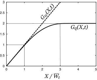
Figure 2: Comparison of the work fluctuation theorem and the heat fluctuation theorem by plotting the function $G_{w}(X,t)$ for the work distribution and the function $G_{q}(X,t)$ for the heat distribution as functions of a scaled $X/\overline{W}_{t}$ in the long time limit $t\rightarrow+\infty$. Here, we used the asymptotic forms (133) and (135) of the work distribution function and the heat distribution function, respectively, in the case of $\overline{W}_{t}=70$. In the small $X$ region ($0\leq X/\overline{W}_{t}\leq 1$), the values of the two functions $G_{w}(X,t)$ and $G_{q}(X,t)$ appear to be consistent with $G_{w}(X,t)=G_{q}(X,t)$, while $G_{w}(X,t)$ is $X/\overline{W}_{t}$ and $G_{q}(X,t)$ is 2 in the large $X$ region ($3\leq X/\overline{W}_{t}\leq+\infty$) in the long time limit.

Now, we introduce the fluctuation functions $G_{w}(W,t)$ and $G_{q}(Q,t)$ defined by

$$G_{w}(W,t) \equiv \frac{1}{\overline{W}_{t}}\ln\frac{P_{w}(W,t)}{P_{w}(-W,t)},$$ (136)

$$G_{q}(Q,t) \equiv \frac{1}{\overline{W}_{t}}\ln\frac{P_{q}(Q,t)}{P_{q}(-Q,t)}$$ (137)

for the work distribution function $P_{w}(W,t)$ and the heat distribution function $P_{q}(Q,t)$. By Eq. (133) the function $G_{w}(W,t)$ is given simply by $G_{w}(W,t)\stackrel{{\scriptstyle t\rightarrow+\infty}}{{\sim}}W/\overline{W}_{t}$ in the long time limit, characterizing the work fluctuation theorem in a proper way to compare it with the heat fluctuation theorem characterized by the function $G_{q}(Q,t)$. In Fig. 2 the functions $G_{w}(W,t)$ (broken line) and $G_{q}(Q,t)$ (solid line) are plotted as functions of $X/\overline{W}_{t}$ ($X=W$ or $Q$) using Eqs. (133) and (135) in the case of $\overline{W}_{t}=70$. In this figure we plotted only in the positive region of $W$ and $Q$, because their values in the negative region is simply given by $G_{w}(-W,t)=-G_{w}(W,t)$ and $G_{q}(-Q,t)=-G_{q}(Q,t)$. It is clear from Fig. 2 that the values of the functions $G_{w}(X,t)$ and $G_{q}(X,t)$ will coincide with each other for small $W$ and $Q$ for $\overline{W}_{t}\rightarrow+\infty$, i.e. $t\rightarrow+\infty$, meaning that the heat fluctuation theorem coincides with the work fluctuation theorem in this region. The difference between the heat and work fluctuation theorems appears in the large values of the argument, where the function $G_{w}(W,t)$ remains $W/\overline{W}_{t}$, while the function $G_{q}(Q,t)$ takes the constant value $2$ for $Q/\overline{W}_{t}>3$ in the long time limit. For further details, we refer to Ref. ZC04 .

VII Inertial Effects

So far, we have concentrated our discussions to the over-damped case and have neglected inertial effects. A generalization of our discussions to the ones including the inertia is almost straightforward. One of the features caused by introducing inertia is a kinetic term in the equilibrium and nonequilibrium steady state distribution functions. This kinetic term depends on the frame one uses, namely the comoving frame or the laboratory frame, respectively. The inertial force, like d’Alembert’s force, also appears as an inertial effect. In this section we discuss briefly these effects beyond the over-damped case.

The Langevin equation including inertia is expressed as Eq. (1) in the laboratory frame. Like in the over-damped case, we can convert Eq. (1) for the laboratory frame to

$$m\frac{d^{2}y_{t}}{dt^{2}}=-\alpha\frac{dy_{t}}{dt}-\kappa\left(y_{t}+v\tau\right)+\zeta_{t}$$ (138)

for the comoving frame by Eq. (5). Equation (138) reduces to Eq. (6) for the over-damped case when $md^{2}y_{t}/dt^{2}=0$.

We introduce a canonical-like distribution function as

$$f_{eq}^{(\vartheta)}(\dot{y},y)\equiv\Xi^{(\vartheta)}{}^{-1}\exp\left[-\beta\mathcal{H}\left(\dot{y}+\vartheta v,y\right)\right]$$ (139)

where $\dot{y}$ is the time-derivative of $y$ and $\mathcal{H}\left(\dot{y},y\right)$ is defined by

$$\mathcal{H}\left(\dot{y},y\right)\equiv m\dot{y}^{2}/2+\kappa y^{2}/2,$$ (140)

and $\Xi^{(\vartheta)}$ is the normalization constant for the distribution function $f_{eq}^{(\vartheta)}(\dot{y},y)$. It is important to note that the particle velocity depends on the frame, and is given by $\dot{y}$ for the comoving frame and by $\dot{x}(=\dot{y}+v)$ for the laboratory frame. For that reason, the canonical distribution function $f_{eq}^{(\vartheta)}(\dot{y},y)$ including the kinetic energy depends on the frame, so that $f_{eq}^{(0)}(\dot{y},y)$ for $\vartheta=0$ refers to the comoving frame and $f_{eq}^{(1)}(\dot{y},y)$ for $\vartheta=1$ refers to the laboratory frame.

By a way similar to the over-damped case, the functional probability density for path $\{y_{s}\}_{s\in[t_{0},t]}$ is given by $\exp[\int_{t_{0}}^{t}ds\;L^{(v)}(\ddot{y}_{s},\dot{y}_{s},y_{s})]$ with the Lagrangian function

$$L^{(v)}\!\left(\ddot{y}_{s},\dot{y}_{s},y_{s}\right)\equiv-\frac{1}{4D}\left(\dot{y}_{s}+\frac{1}{\tau}y_{s}+v+\frac{m}{\alpha}\ddot{y}_{s}\right)^{2}$$ (141)

using $\ddot{y}_{s}\equiv d^{2}y_{s}/ds^{2}$. The Lagrangian function (141) becomes the Lagrangian function (18) in the over-damped case, where $m\ddot{y}_{s}=0$. Using Eqs. (139) and (141) we obtain

$$e^{-\beta\int_{t_{0}}^{t}ds\;\Lambda_{\pm}(\ddot{y}_{s},\dot{y}_{s},y_{s};\vartheta)v}e^{\int_{t_{0}}^{t}ds\;L^{(v)}\!\left(\ddot{y}_{s},\dot{y}_{s},y_{s}\right)}f_{eq}^{(\vartheta)}\!\left(\dot{y}_{0},y_{0}\right)$$

$$\hskip 22.76228pt=f_{eq}^{(\vartheta)}\!\left(\dot{y}_{t},y_{t}\right)e^{\int_{t_{0}}^{t}ds\;L^{(\pm v)}\left(\ddot{y}_{s},-\dot{y}_{s},y_{s}\right)}$$ (142)

where $\dot{y}_{0}=\dot{y}_{t_{0}}$, and $\Lambda_{\pm}(\ddot{y}_{s},\dot{y}_{s},y_{s};\vartheta)$ is a modified “force” defined by

$$\Lambda_{\pm}(\ddot{y}_{s},\dot{y}_{s},y_{s};\vartheta) \equiv -\kappa y_{s}\frac{1\mp 1}{2}-\alpha\dot{y}_{s}\frac{1\pm 1}{2}$$ (143)

$$\hskip 22.76228pt-m\ddot{y}_{s}\left(\frac{1\mp 1}{2}-\vartheta\right).$$

Equation (142) may be regarded as a nonequilibrium detailed balance relation for the case of a potential force, friction and inertia. [See Appendix D for a derivation of Eq. (142).] Moreover, the signs $\pm$ in Eq. (142) correspond to the case of work ($-1$), discussed in IV and that of energy loss by friction ($+1$), respectively, discussed in Sec. V, and are due to the $\pm v$ signs of the Lagrangian $L^{(\pm v)}(\ddot{y}_{s},-\dot{y}_{s},y_{s})$ on the right-hand side of Eq. (142). It should be noted that the first, second and third terms on the right-hand side of Eq. (143) are regarded as the harmonic force, the friction force, and the inertial (d’Alembert-like) force, respectively.

Table 1: Four kinds of fluctuation theorems corresponding to four forces in the case including inertial effects. Here, $\vartheta=0$ ($\vartheta=1$) is for the case of the comoving frame (the laboratory frame), and $\pm v$ is the velocity appearing in the Lagrangian function $L^{(\pm v)}(\ddot{y}_{s},-\dot{y}_{s},y_{s})$ on the right-hand side of the nonequilibrium detailed balance relation (142).

Frame ($\vartheta$)	$\hskip 14.22636pt\pm v\hskip 14.22636pt$	Force $\Lambda$	Fluctuation Theorem
Comoving ($0$)	$-v$	$\Lambda_{-}(\ddot{y},\dot{y},y;0)=-\kappa y-m\ddot{y}$	$\textstyle\frac{\mathcal{P}_{-}^{(0)}(\mathcal{W},t)}{\mathcal{P}_{-}^{(0)}(-\mathcal{W},t)}=\exp(\mathcal{W})$
Comoving ($0$)	$+v$	$\Lambda_{+}(\ddot{y},\dot{y},y;0)=-\alpha\dot{y}$	$\textstyle\frac{\mathcal{P}_{+}^{(0)}(\mathcal{W},t)}{\mathcal{P}_{+}^{(0)}(-\mathcal{W},t)}=\exp(\mathcal{W})$
Laboratory ($1$)	$-v$	$\Lambda_{-}(\ddot{y},\dot{y},y;1)=-\kappa y$	$\textstyle\frac{\mathcal{P}_{-}^{(1)}(\mathcal{W},t)}{\mathcal{P}_{-}^{(1)}(-\mathcal{W},t)}=\exp(\mathcal{W})$
Laboratory ($1$)	$+v$	$\Lambda_{+}(\ddot{y},\dot{y},y;1)=-\alpha\dot{y}+m\ddot{y}$	$\textstyle\frac{\mathcal{P}_{+}^{(1)}(\mathcal{W},t)}{\tilde{\mathcal{P}}_{+}^{(1)}(-\mathcal{W},t)}=\exp(\mathcal{W})$

Now, we introduce the dimensionless modified “work” rate $\beta\Lambda_{\pm}(\ddot{y},\dot{y},y;\vartheta)v$ and its distribution function $\mathcal{P}_{\pm}^{(\vartheta)}(\mathcal{W},t)$ as

$$\mathcal{P}_{\pm}^{(\vartheta)}(\mathcal{W},t)=\left\langle\!\!\!\left\langle\delta\left(\mathcal{W}-\beta\int_{t_{0}}^{t}ds\;\Lambda_{\pm}(\ddot{y},\dot{y},y;\vartheta)v\right)\right\rangle\!\!\!\right\rangle_{t}$$ (144)

where $\left\langle\!\!\!\left\langle\cdots\right\rangle\!\!\!\right\rangle_{t}$ is the functional average in the inertia case, like the one given by Eq. (72). Here, we remark that $\mathcal{W}$ in Eq. (144) differs from the work $\mathcal{W}_{t}^{(v)}(\{y_{s}\})$ defined by Eq. (33). In a way similar to derive Eqs. (77) and (115) in the over-damped case, it follows that the distribution function $\mathcal{P}_{\pm}^{(\vartheta)}(\mathcal{W},t)$ satisfies the transient fluctuation theorem

$$\frac{\mathcal{P}_{\pm}^{(\vartheta)}(\mathcal{W},t)}{\tilde{\mathcal{P}}_{\pm}^{(\vartheta)}(-\mathcal{W},t)}=\exp(\mathcal{W})$$ (145)

under the condition that the initial distribution at time $t_{0}$ is given by the $f_{eq}^{(\vartheta)}(\dot{y},y)$. Here, the distribution $\tilde{\mathcal{P}}_{\pm}^{(\vartheta)}(\mathcal{W},t)$ is defined by

$$\tilde{\mathcal{P}}_{\pm}^{(\vartheta)}(\mathcal{W},t)$$

$$=\left\langle\!\!\!\left\langle\delta\left(\mathcal{W}-\beta\int_{t_{0}}^{t}ds\;\Lambda_{\pm}(\ddot{y},\dot{y},y;(-1)^{\frac{1\pm 1}{2}}\vartheta)v\right)\right\rangle\!\!\!\right\rangle_{t},$$

(146)

and is simply given by

$$\tilde{\mathcal{P}}_{+}^{(0)}(\mathcal{W},t) = \mathcal{P}_{+}^{(0)}(\mathcal{W},t),$$ (147)

$$\tilde{\mathcal{P}}_{-}^{(\vartheta)}(\mathcal{W},t) = \mathcal{P}_{-}^{(\vartheta)}(\mathcal{W},t)$$ (148)

in these special cases, and in order to derive Eq. (145) we also used the relations $L^{(v)}\!\left(\ddot{y}_{s},\dot{y}_{s},y_{s}\right)=L^{(-v)}\!\left(-\ddot{y}_{s},-\dot{y}_{s},-y_{s}\right)$, $\Lambda_{\pm}(\ddot{y}_{s},\dot{y}_{s},y_{s};\vartheta)=-\Lambda_{\pm}(-\ddot{y}_{s},-\dot{y}_{s},-y_{s};\vartheta)$ and

$$\Lambda_{\pm}(\ddot{y}_{s},\dot{y}_{s},y_{s};\vartheta)v=-\Lambda_{\pm}(\ddot{y}_{s},-\dot{y}_{s},y_{s};(-1)^{\frac{1\pm 1}{2}}\vartheta)(\pm v).$$

It may be noted that the two terms $-\alpha\dot{y}$ and $m\ddot{y}$ for the force $\Lambda_{+}(\ddot{y}_{s},\dot{y}_{s},y_{s};1)$ have different time-reversal properties than the other forces $\Lambda_{+}(\ddot{y}_{s},\dot{y}_{s},y_{s};0)$ and $\Lambda_{+}(\ddot{y}_{s},\dot{y}_{s},y_{s};\vartheta)$.

From Eq. (145) we derived four different fluctuation theorems corresponding to the cases $(\vartheta,\pm v)=(0,-v)$, $(1,-v)$, $(0,v)$, and $(1,v)$, where $\pm v$ is the velocity appearing in the Lagrangian function $L^{(\pm v)}(\ddot{y}_{s},-\dot{y}_{s},y_{s})$ on the right-hand side of the nonequilibrium detailed balance relation (142). We summarize these four fluctuation theorems in Table 1. In the last line of this table, appearance of the function $\tilde{\mathcal{P}}_{+}^{(1)}(-\mathcal{W},t)$ for the case of $(\vartheta,\pm v)=(1,v)$ is due to the different behavior with respect to time-reversal of the two terms $-\alpha\dot{y}$ and $m\ddot{y}$ composing the modified force $\Lambda_{+}(\ddot{y}_{s},\dot{y}_{s},y_{s};1)$, while in all the other cases in Table 1 the modified forces have the unique behavior under time-reversal.

VIII Conclusions and Remarks

In this paper we discussed a generalization of Onsager-Machlup’s fluctuation theory to nonequilibrium steady states and fluctuation theorems based on nonequilibrium detailed balance relations. To that end, we used a model which consists of a Brownian particle confined by a harmonic potential which is dragged with a constant velocity through a heat reservoir. This model is described by a Langevin equation, which is a simple and exactly-solvable nonequilibrium steady state model. Our basic analytical approach is a functional integral technique, which was used in Onsager and Machlup’s original work and is effective to discuss fluctuation theorems treating quantities expressed as functionals, for example, work and heat.

First, we gave an expression of the transition probability in terms of a Lagrangian function which can be written as a sum of an entropy production rate and two dissipation functions. There is a difference, though with the similar result of Onsager and Machlup’s original papers OM53 ; MO53 , in that now the entropy production rate and one of the two dissipation functions - and consequently also the Lagrangian function - depend on the dragging velocity $v$ leading to nonequilibrium steady state effects. From this property of the Lagrangian function, we constructed a nonequilibrium steady state thermodynamics by obtaining the second law of thermodynamics and the energy conservation law which involves fluctuating heat, work and an internal potential energy difference. We also discussed Onsager’s principle of minimum energy dissipation and the most probable path approximating the transition probability of the particle position. This approach is different from another attempt for an Onsager-Machlup theory for nonequilibrium steady states BSG01 ; BSG02 , where a nonlinear diffusion equation is applied to models like an exclusion model and a boundary driven zero range model. Instead, we use a stochastic model described by a Langevin equation, so that our results automatically include those of Onsager and Machlup’s original works by taking a specific equilibrium value, $v=0$, for the nonequilibrium parameter $v$, and relax Onsager and Machlup’s variable $\alpha$ and $\dot{\alpha}$ in Refs. OM53 ; MO53 to our variables $x$ and $\dot{x}$, respectively.

Second, we derived nonequilibrium detailed balance relations from the Lagrangian function to obtain not only the well-known fluctuation theorem for work but also another fluctuation theorem for energy loss by friction. We also indicated the derivation of the extended fluctuation theorem for heat by carrying out explicitly the relevant functional integral and then using Refs. ZC03a ; ZC04 . In addition, we gave a simple argument for the heat fluctuation theorem in the long time limit. Finally, we discussed briefly the effects of inertia, and obtained four different fluctuation theorems related to a potential force, a friction force and d’Alembert-like (or inertial) force for the comoving frame or the laboratory frame.

In the remaining of this section, we give remarks for the contents in the main text of this paper.

1) In this paper, we have emphasized a close connection between nonequilibrium detailed balance relations and fluctuation theorems, using a functional integral approach. It may be noted that in some of past works concepts of detailed balances have been mentioned for formal derivations of fluctuation theorems in various different contexts, implicitly or explicitly ECM93 ; K98 ; LS99 ; C99 ; C00 ; CCJ06 . However, we should keep in mind that a generalization of the equilibrium detailed balance to nonequilibrium states is not unique, as shown in this paper [cf. Eq. (61) and (94)]. As a remark related to this point, we should notice that even if the equilibrium detailed balance condition is violated, but another detailed balance condition for the nonequilibrium steady state still holds, namely, using the nonequilibrium steady state distribution $f_{ss}(y)$ we obtain for the over-damped case:

$$e^{\int_{t_{0}}^{t}ds\;L^{(v)}\!\left(\dot{y}_{s},y_{s}\right)}f_{ss}(y_{0})=f_{ss}(y_{t})\;e^{\int_{t_{0}}^{t}ds\;L^{(v)}\!\left(-\dot{y}_{s},y_{s}\right)},\;\;\;$$ (150)

by Eqs. (18), (26) and (27), or equivalently ${F}\!(\begin{array}[]{c}\!\!\scriptstyle{y_{t}}\!\!\\ \!\!\scriptstyle{t}\!\!\end{array}|\begin{array}[]{c}\!\!\scriptstyle{y_{0}}\!\!\\ \!\!\scriptstyle{t_{0}}\!\!\end{array})f_{ss}(y_{0})={F}\!(\begin{array}[]{c}\!\!\scriptstyle{y_{0}}\!\!\\ \!\!\scriptstyle{t}\!\!\end{array}|\begin{array}[]{c}\!\!\scriptstyle{y_{t}}\!\!\\ \!\!\scriptstyle{t_{0}}\!\!\end{array})f_{ss}(y_{t})$. Here, it is essential to note that on the right-hand side of Eq. (150) we do not change the sign of the dragging velocity $v$ although we change the sign of the particle velocity $\dot{y}_{s}$ in the comoving frame. We emphasize that here, there is no additional multiplying factors like $\exp[-\beta\mathcal{W}_{t}^{(v)}(\{y_{s}\})]$ as in Eq. (61) or $\exp[-\beta\mathcal{R}_{t}^{(v)}(y_{t},y_{0})]$ as in Eq. (94). As a consequence we have been unable to derive fluctuation theorems from Eq. (150). Since we chose the equilibrium state as the reference state for the detailed balance in this paper, our interest was mainly the work to maintain the system in a nonequilibrium steady state, i.e. the work necessary to keep the system from going to the equilibrium state. In this sense, we note that the reference state is arbitrary, for example, if we are interested in the work to go from one nonequilibrium state to another nonequilibrium state. In general, the modification of the detailed balance relation based on an arbitrary reference distribution function $f_{ref}(y)$ can be expressed as

$$e^{-\beta Y_{t}(\{y_{s}\})}e^{\int_{t_{0}}^{t}ds\;L^{(v)}\!\left(\dot{y}_{s},y_{s}\right)}f_{ref}(y_{0})$$

$$\hskip 22.76228pt=f_{ref}(y_{t})\;e^{\int_{t_{0}}^{t}ds\;L^{(-v)}\!\left(-\dot{y}_{s},y_{s}\right)}$$ (151)

where $Y_{t}(\{y_{s}\})$ is the functional defined by

$$Y_{t}(\{y_{s}\})\equiv\mathcal{Q}^{(v)}_{t}(\{y_{s}\})+\beta^{-1}\ln\frac{f_{ref}(y_{0})}{f_{ref}(y_{t})}.$$ (152)

Choosing $f_{ref}(y)=f_{eq}(y)$, Eq. (151) leads to Eq. (61). We can also get a generalization of Eq. (94) for an arbitrary reference distribution function $f_{ref}(y)$. An analogous quantity to $Y_{t}(\{y_{s}\})$ is in Ref. ES02 for a thermostated system with deterministic dynamics.

2) From Eq. (150) we derive

$$\int_{t_{0}}^{t}ds\;L^{(v)}\!\left(\dot{y}_{s},y_{s}\right)+\tilde{S}_{ss}(y_{0})/k_{B}$$

$$\hskip 22.76228pt=\int_{t_{0}}^{t}ds\;L^{(v)}\!\left(-\dot{y}_{s},y_{s}\right)+\tilde{S}_{ss}(y_{t})/k_{B}$$ (153)

where $\tilde{S}_{ss}(y)$ is defined by $\tilde{S}_{ss}(y)\equiv k_{B}\ln f_{ss}(y)$. An identity like Eq. (153) is called an Onsager-Machlup symmetry BSG01 ; BSG02 ; G02 , and is used to discuss macroscopic properties of nonequilibrium steady states. Using Eq. (153) we can also obtain an expression like

$$\frac{\exp\left[\int_{t_{0}}^{t}ds\;L^{(v)}\!\left(\dot{y}_{s},y_{s}\right)\right]}{\exp\left[\int_{t_{0}}^{t}ds\;L^{(v)}\!\left(-\dot{y}_{s},y_{s}\right)\right]}=\exp\left[\beta\tilde{Q}_{ss}(t,t_{0})\right]$$ (154)

with $\tilde{Q}_{ss}(t,t_{0})\equiv T[\tilde{S}_{ss}(y_{t})-\tilde{S}_{ss}(y_{0})]$. On the other hand, it can be shown from Eqs. (27), (34) and (61) [or from Eq. (151)] that

$$\frac{\exp\left[\int_{t_{0}}^{t}ds\;L^{(v)}\!\left(\dot{y}_{s},y_{s}\right)\right]}{\exp\left[\int_{t_{0}}^{t}ds\;L^{(-v)}\!\left(-\dot{y}_{s},y_{s}\right)\right]}=\exp\left[\beta\mathcal{Q}^{(v)}_{t}(\{y_{s}\})\right]$$ (155)

using the heat $\mathcal{Q}^{(v)}_{t}(\{y_{s}\})$ of Eq. (32). Note that Eq. (155) is consistent with the heat $\mathcal{Q}^{(v)}_{t}(\{y_{s}\})$ appearing in our energy conservation law (34), in contrast to Eq. (154) in which the quantity $\tilde{Q}_{ss}(t,t_{0})$ does not have such a correspondence with the heat. Thus we will restrict ourselves in the following to Eq. (155). As we discussed in Sec. II, the term $\exp[\int_{t_{0}}^{t}ds\;L^{(v)}\!(\dot{y}_{s},y_{s})]$ appearing in the numerator on the left-hand side of Eq. (155) is the probability functional of the forward path $\{y_{s}\}_{s\in[t_{0},t]}$. On the other hand, the denominator on the left-hand side of Eq. (155) is the probability functional of the corresponding time-reversed path with the dragging velocity $-v$. Therefore, Eq. (155) implies that the logarithm of the ratio of such forward and backward probability functionals is given by the heat multiplied by the inverse temperature. In this sense it is tempting to claim Eq. (155) as a relation leading to a fluctuation theorem ND04 ; K05 ; IP06 . However, it is important to distinguish Eq. (155) from the fluctuation theorems discussed in the main text of this paper. First of all, although it is related to the heat, Eq. (155) has a form rather close to a relation leading to the conventional fluctuation theorems like Eqs. (77) and (115), which are different from the extended form for the heat fluctuation theorem discussed in Sec. VI. Similarly, although one may regard Eq. (155) as a nonequilibrium detailed balance relation for heat, a derivation of the extended fluctuation theorem for heat from a nonequilibrium detailed balance relation remains an open problem. We should also notice that no initial condition dependence appears in Eq. (155), so that we cannot discuss directly, for example, a difference between the transient fluctuation theorem and the steady state fluctuation theorem for them from Eq. (155).

3) Although the nonequilibrium detailed balance relations, like Eq. (61), (94) or (151), play an essential role to derive the fluctuation theorem, it is important to note that some properties of the fluctuation theorem cannot be discussed by it. Basically, the nonequilibrium detailed balance relation can lead directly to the so-called transient fluctuation theorems, which are identically satisfied for any time CG99 , but this relation does not say what happens to fluctuation theorems if we change the initial condition (like the equilibrium distribution) to another (like the nonequilibrium steady state discussed in the steady state fluctuation theorem). The transient fluctuation theorem can be different from the steady state fluctuation theorem for some quantities, even in the long time limit. As an example for such a difference, we showed in this paper that the energy loss by friction satisfies the transient fluctuation theorem but does not satisfy the steady state fluctuation theorem.

We have discussed an initial condition dependence of fluctuation theorems by carrying out functional integrals to obtain distribution functions explicitly, and showed that the work distribution function has an asymptotic form satisfying the work fluctuation theorem, independent of the initial distribution, while the friction-loss distribution function depends on the initial condition even in the long time limit. This difference between the work and the friction-loss might come from the fact that the work is given by a time-integral of the particle position so that its contribution near the initial time can be neglected in the long time limit, while the energy loss by friction is given by the particle position at the initial and final times only. A systematic way to investigate whether a fluctuation theorem is satisfied for any initial condition without calculating a distribution function, remains an open problem noteHeat .

4) Finally we note that the analogy of the Brownian particle case, discussed here, and the electric circuit case should persist not only in the over-damped case (as shown in ZCC04 ) but also in the case including inertia. In that case, one has to add the self-induction $L_{0}$ of the electric circuit, as the corresponding quantity of the mass $m$ of the Brownian particle. This will add the correspondence of $m$ and $L_{0}$ to Table I in Ref. ZCC04 . Then, the fluctuation theorems in Table 1 in Sec. VII of this paper can, by using the extended analogy described above, also be used for electric circuits, and might be experimentally accessible (cf. GC05 ).

Appendix A Transition Probability using a Functional Integral Technique

In this Appendix, we outline a derivation of the transition probability (17) for the stochastic process described by the Langevin equation (6).

First, we translate the Langevin equation (6) into the corresponding Fokker-Planck equation. It can be done using the Kramers-Moyal expansion technique K92 ; R89 , and we obtain the Fokker-Planck equation

$$\frac{\partial f(y,t)}{\partial t}=\hat{\mathcal{L}}f(y,t)$$ (156)

for the distribution function $f(y,t)$ of the particle position $y$ at time $t$. Here, $\hat{\mathcal{L}}$ is the Fokker-Planck operator defined by

$$\hat{\mathcal{L}}\equiv\frac{\partial}{\partial y}\left(\frac{y+v\tau}{\tau}+D\frac{\partial}{\partial y}\right)$$ (157)

with $D\equiv 1/(\alpha\beta)$.

The transition probability ${F}\!(\begin{array}[]{c}\!\!\scriptstyle{y}\!\!\\ \!\!\scriptstyle{t+\Delta t}\!\!\end{array}|\begin{array}[]{c}\!\!\scriptstyle{y^{\prime}}\!\!\\ \!\!\scriptstyle{t}\!\!\end{array})$ from $y^{\prime}$ at time $t$ to $y$ at time $t+\Delta t$ is given by

$${F}\!\left(\begin{array}[]{c}\!\!y\!\!\\ \!\!t+\Delta t\!\!\end{array}\right|\left.\begin{array}[]{c}\!\!y^{\prime}\!\!\\ \!\!t\!\!\end{array}\right) = e^{\hat{\mathcal{L}}\Delta t}\delta(y-y^{\prime})$$

$$= \left[1+\hat{\mathcal{L}}\Delta t+\mathcal{O}\left(\Delta t^{2}\right)\right]\delta\left(y-y^{\prime}\right)$$

$$= \left(1+\Delta t\frac{\partial}{\partial y}\frac{y^{\prime}+v\tau}{\tau}+D\Delta t\frac{\partial^{2}}{\partial y^{2}}\right)\delta\left(y-y^{\prime}\right)+\mathcal{O}\left(\Delta t^{2}\right)$$

$$= \frac{1}{2\pi}\int_{-\infty}^{+\infty}d\lambda\;\left(1+\Delta t\frac{y^{\prime}+v\tau}{\tau}\frac{\partial}{\partial y}+D\Delta t\frac{\partial^{2}}{\partial y^{2}}\right)\exp\left[i\lambda(y-y^{\prime})\right]+\mathcal{O}\left(\Delta t^{2}\right)$$

$$= \frac{1}{2\pi}\int_{-\infty}^{+\infty}d\lambda\;\exp\left[-D\Delta t\lambda^{2}+i\Delta t\left(\frac{y-y^{\prime}}{\Delta t}+\frac{y^{\prime}+v\tau}{\tau}\right)\lambda\right]+\mathcal{O}\left(\Delta t^{2}\right)$$

$$= \frac{1}{\sqrt{4\pi D\Delta t}}\exp\left[-\frac{1}{4D}\left(\frac{y-y^{\prime}}{\Delta t}+\frac{y^{\prime}+v\tau}{\tau}\right)^{2}\Delta t\right]+\mathcal{O}(\Delta t^{2})$$ (163)

where we used $y\delta\left(y-y^{\prime}\right)=y^{\prime}\delta\left(y-y^{\prime}\right)$. On the other hand, using the Chapman-Kolmogorov equation K92 , the transition probability for a finite time interval $t-t_{0}$ is expressed as

$${F}\!\left(\begin{array}[]{c}\!\!y_{t}\!\!\\ \!\!t\!\!\end{array}\right|\left.\begin{array}[]{c}\!\!y_{0}\!\!\\ \!\!t_{0}\!\!\end{array}\right) = \lim_{N\rightarrow+\infty}\int dy_{N-1}\int dy_{N-2}\cdots\int dy_{1}\;{F}\!\left(\begin{array}[]{c}\!\!y_{t}\!\!\\ \!\!t\!\!\end{array}\right|\left.\begin{array}[]{c}\!\!y_{N-1}\!\!\\ \!\!t_{N-1}\!\!\end{array}\right){F}\!\left(\begin{array}[]{c}\!\!y_{N-1}\!\!\\ \!\!t_{N-1}\!\!\end{array}\right|\left.\begin{array}[]{c}\!\!y_{N-2}\!\!\\ \!\!t_{N-2}\!\!\end{array}\right)\cdots{F}\!\left(\begin{array}[]{c}\!\!y_{1}\!\!\\ \!\!t_{1}\!\!\end{array}\right|\left.\begin{array}[]{c}\!\!y_{0}\!\!\\ \!\!t_{0}\!\!\end{array}\right)$$ (180)

with $t_{n}\equiv t_{0}+n\Delta t_{N}$, $n=1,2,\cdots,N$, $\Delta t_{N}\equiv(t-t_{0})/N$, $t_{N}=t$. Inserting the expression (163) for the transition probability in a short time interval $\Delta t=\Delta t_{N}$ into Eq. (180) we obtain Eq. (17) with the functional integral (19).

Appendix B Fluctuation Theorem for Work

In this Appendix, we show the relation $\mathcal{E}_{w}^{(v)}(\lambda,t)=\mathcal{E}_{w}^{(-v)}(1-\lambda,t)$, therefore Eq. (77). We also give a derivation of Eq. (77) from Eq. (76).

From Eq. (74) with the functional average (72) we derive

$$\mathcal{E}_{w}^{(v)}(\lambda,t) = \int dy_{t}\!\int_{y_{0}}^{y_{t}}\mathcal{D}y_{s}\!\int dy_{0}\;e^{\int_{t_{0}}^{t}ds\;L^{(v)}\!\left(\dot{y}_{s},y_{s}\right)}f(y_{0},t_{0})\;e^{-\lambda\beta\mathcal{W}_{t}^{(v)}(\{y_{s}\})}$$ (181)

$$= \int dy_{t}\!\int_{y_{0}}^{y_{t}}\mathcal{D}y_{s}\!\int dy_{0}\;f_{eq}(y_{t})\;e^{\int_{t_{0}}^{t}ds\;L^{(-v)}\!\left(-\dot{y}_{s},y_{s}\right)}\;e^{\beta\mathcal{W}_{t}^{(v)}(\{y_{s}\})}\frac{1}{f_{eq}(y_{0})}\;f(y_{0},t_{0})\;e^{-\lambda\beta\mathcal{W}_{t}^{(v)}(\{y_{s}\})}$$

$$= \int dy_{0}\!\int_{y_{0}}^{y_{t}}\mathcal{D}y_{s}\!\int dy_{t}\;e^{\int_{t_{0}}^{t}ds\;L^{(-v)}\!\left(-\dot{y}_{s},y_{s}\right)}f_{eq}(y_{t})\;e^{-(1-\lambda)\beta\mathcal{W}_{t}^{(-v)}(\{y_{s}\})}$$

$$= \int dy_{t}\!\int_{y_{0}}^{y_{t}}\mathcal{D}y_{s}\!\int dy_{0}\;e^{\int_{t_{0}}^{t}ds\;L^{(-v)}\!\left(\dot{y}_{s},y_{s}\right)}f_{eq}(y_{0})\;e^{-(1-\lambda)\beta\mathcal{W}_{t}^{(-v)}(\{y_{s}\})}$$ (182)

$$= \mathcal{E}_{w}^{(-v)}(1-\lambda,t)$$ (183)

where we used Eqs. (61) and $\mathcal{W}_{t}^{(-v)}(\{y_{s}\})=-\mathcal{W}_{t}^{(v)}(\{y_{s}\})$, and the assumption $f(y_{0},t_{0})=f_{eq}(y_{0})$. Here, in the transformation from Eq. (181) to Eq. (182) we changed the integral variables as $y_{s}\rightarrow y_{t+t_{0}-s}$ (so that $\dot{y}_{s}\rightarrow-\dot{y}_{s}$, $y_{t}\rightarrow y_{0}$ and $y_{0}\rightarrow y_{t}$). Therefore, we obtain $\mathcal{E}_{w}^{(v)}(\lambda,t)=\mathcal{E}_{w}^{(-v)}(1-\lambda,t)$, whose combination with Eq (75) leads to Eq. (76).

Moreover, from Eqs. (73) and (76) we derive

$$P_{w}(W,t) = \frac{1}{2\pi}\int_{-\infty}^{+\infty}d\lambda\;e^{i\lambda W}\mathcal{E}_{w}^{(v)}(1-i\lambda)$$ (184)

$$= \frac{1}{2\pi}\int_{-\infty-i}^{+\infty-i}d\mu\;e^{(1-i\mu)W}\mathcal{E}_{w}^{(v)}(i\mu)$$

$$= e^{W}\frac{1}{2\pi}\int_{-\infty}^{+\infty}d\mu\;e^{i\mu(-W)}\mathcal{E}_{w}^{(v)}(i\mu)$$ (185)

$$= e^{W}P_{w}(-W,t)$$ (186)

with $\mu\equiv-\lambda-i$. Here, in the transformation from Eq. (184) to Eq. (185) we used the fact that noting Eq. (74) the function $\mathcal{E}_{w}^{(v)}(i\mu)\exp[(1-i\mu)W]$ appearing in Eq. (184) does not have any pole in the complex region for $\mbox{Im}\{\mu\}\in[0,1]$ (here $\mbox{Im}\{\mu\}$ is the imaginary part of $\mu$). Using Eq. (186) we obtain Eq. (77).

Appendix C Functional Integral Calculation for the Work Distribution

In this Appendix, we give calculation details of Eqs. (81), (83) and (86).

Inserting Eq. (7) and (18) into Eq. (80), we obtain

$$\frac{d^{2}\tilde{y}^{*}\!\!_{s}}{ds^{2}}=\frac{\tilde{y}^{*}\!\!_{s}+(1-2\lambda)v\tau}{\tau^{2}}$$ (187)

where we used the relations $\alpha=\kappa\tau$ and $D=1/(\alpha\beta)$. [Note that Eq. (187) for $\tilde{y}^{*}\!\!_{s}$ is Eq. (46) for $y_{s}^{*}$ except for that Eq. (187) use $(1-2\lambda)v$ instead of $v$ in Eq. (46).] The solution of Eq. (187) is given by

$$\tilde{y}^{*}\!\!_{s}+(1-2\lambda)v\tau=\tilde{A}_{1}\exp\left(\frac{s}{\tau}\right)+\tilde{A}_{2}\exp\left(-\frac{s}{\tau}\right).$$ (188)

Here, $\tilde{A}_{1}$ and $\tilde{A}_{2}$ are constants determined by the conditions $\tilde{y}^{*}\!\!_{t}=y_{t}$ and $\tilde{y}^{*}\!\!_{0}(=\tilde{y}^{*}\!\!_{t_{0}})=y_{0}$, namely

$$\left(\begin{array}[]{c}y_{0}+(1-2\lambda)v\tau\\ y_{t}+(1-2\lambda)v\tau\end{array}\right)$$ (191)

$$\hskip 22.76228pt=\left(\begin{array}[]{cc}\exp\left(\frac{t_{0}}{\tau}\right)&\exp\left(-\frac{t_{0}}{\tau}\right)\\ \exp\left(\frac{t}{\tau}\right)&\exp\left(-\frac{t}{\tau}\right)\end{array}\right)\left(\begin{array}[]{c}\tilde{A}_{1}\\ \tilde{A}_{2}\end{array}\right).$$ (196)

Solving Eq. (196) for $\tilde{A}_{1}$ and $\tilde{A}_{2}$ we obtain

$$\left(\begin{array}[]{c}\tilde{A}_{1}\\ \tilde{A}_{2}\end{array}\right)=\left(\begin{array}[]{c}A_{t-t_{0}}^{((1-2\lambda)v)}(y_{t},y_{0})\exp\left(-\frac{t}{\tau}\right)\\ A_{-(t-t_{0})}^{((1-2\lambda)v)}(y_{t},y_{0})\exp\left(\frac{t}{\tau}\right)\end{array}\right)$$ (201)

with the function $A_{t-t_{0}}^{(v)}(y_{t},y_{0})$ defined by Eq. (82). Further, we note

$$A_{-(t-t_{0})}^{(v)}(y_{t},y_{0})=A_{t-t_{0}}^{(v)}(y_{0},y_{t})b_{t}.$$ (202)

which can be shown from Eq. (82). Using Eqs. (188), (201) and (202) we obtain Eq. (81).

Noting that the Lagrangian function $L^{(v)}(\dot{y}_{s},y_{s})$ defined by Eq. (18) and the work rate $\dot{\mathcal{W}}^{(v)}(y_{t})$ given by Eq. (7) are the second order to $y_{t}$ and $\dot{y}_{s}$ at most, we obtain

$$\int_{t_{0}}^{t}ds\left[L^{(v)}(\dot{y}_{s},y_{s})-\lambda\beta\dot{W}(y_{s})\right]$$

$$\hskip 22.76228pt=\int_{t_{0}}^{t}ds\left[L^{(v)}(\dot{\tilde{y}^{*}\!\!}_{s}+\dot{\tilde{z}}_{s},\tilde{y}^{*}\!\!_{s}+\tilde{z}_{s})-\lambda\beta\dot{W}(\tilde{y}^{*}\!\!_{s}+\tilde{z}_{s})\right]$$

$$\hskip 22.76228pt=\int_{t_{0}}^{t}ds\;\left\{L^{(v)}(\dot{\tilde{y}^{*}\!\!}_{s},\tilde{y}^{*}\!\!_{s})-\lambda\beta\dot{W}(\tilde{y}^{*}\!\!_{s})+\frac{\partial\left[L^{(v)}(\dot{\tilde{y}^{*}\!\!}_{s},\tilde{y}^{*}\!\!_{s})-\lambda\beta\dot{W}(\tilde{y}^{*}\!\!_{s})\right]}{\partial\dot{\tilde{y}^{*}\!\!}_{s}}\dot{\tilde{z}}_{s}\right.$$

$$\hskip 22.76228pt\hskip 22.76228pt\hskip 22.76228pt\left.+\frac{\partial\left[L^{(v)}(\dot{\tilde{y}^{*}\!\!}_{s},\tilde{y}^{*}\!\!_{s})-\lambda\beta\dot{W}(\tilde{y}^{*}\!\!_{s})\right]}{\partial\tilde{y}^{*}\!\!_{s}}\tilde{z}_{s}+\frac{1}{2}\frac{\partial^{2}\left[L^{(v)}(\dot{\tilde{y}^{*}\!\!}_{s},\tilde{y}^{*}\!\!_{s})-\lambda\beta\dot{W}(\tilde{y}^{*}\!\!_{s})\right]}{\partial\dot{\tilde{y}^{*}\!\!}_{s}{}^{2}}\dot{\tilde{z}}_{s}^{2}\right.$$

$$\hskip 22.76228pt\hskip 22.76228pt\hskip 22.76228pt\left.+\frac{\partial^{2}\left[L^{(v)}(\dot{\tilde{y}^{*}\!\!}_{s},\tilde{y}^{*}\!\!_{s})-\lambda\beta\dot{W}(\tilde{y}^{*}\!\!_{s})\right]}{\partial\dot{\tilde{y}^{*}\!\!}_{s}\partial\tilde{y}^{*}\!\!_{s}}\dot{\tilde{z}}_{s}\tilde{z}_{s}+\frac{1}{2}\frac{\partial^{2}\left[L^{(v)}(\dot{\tilde{y}^{*}\!\!}_{s},\tilde{y}^{*}\!\!_{s})-\lambda\beta\dot{W}(\tilde{y}^{*}\!\!_{s})\right]}{\partial\tilde{y}^{*}\!\!_{s}{}^{2}}\tilde{z}_{s}^{2}\right\}$$

$$\hskip 22.76228pt=\int_{t_{0}}^{t}ds\;\Biggl{\{}L^{(v)}(\dot{\tilde{y}^{*}\!\!}_{s},\tilde{y}^{*}\!\!_{s})-\lambda\beta\dot{W}(\tilde{y}^{*}\!\!_{s})\left.-\left[\frac{d}{ds}\frac{\partial L^{(v)}(\dot{\tilde{y}^{*}\!\!}_{s},\tilde{y}^{*}\!\!_{s})}{\partial\dot{\tilde{y}^{*}\!\!}_{s}}-\frac{\partial L^{(v)}(\dot{\tilde{y}^{*}\!\!}_{s},\tilde{y}^{*}\!\!_{s})}{\partial\tilde{y}^{*}\!\!_{s}}+\lambda\beta\frac{\partial\dot{W}(\tilde{y}^{*}\!\!_{s})}{\partial\tilde{y}^{*}\!\!_{s}}\right]\tilde{z}_{s}\right.$$

$$\hskip 22.76228pt\hskip 22.76228pt\hskip 22.76228pt-\frac{1}{4D}\left(\dot{\tilde{z}}_{s}^{2}+\frac{2}{\tau}\dot{\tilde{z}}_{s}\tilde{z}_{s}+\frac{1}{\tau^{2}}\tilde{z}_{s}^{2}\right)\Biggr{\}}$$

$$\hskip 22.76228pt=\int_{t_{0}}^{t}ds\;\left[L^{(v)}(\dot{\tilde{y}^{*}\!\!}_{s},\tilde{y}^{*}\!\!_{s})-\lambda\beta\dot{W}(\tilde{y}^{*}\!\!_{s})+L^{(0)}(\dot{\tilde{z}}_{s},\tilde{z}_{s})\right]$$ (203)

using a partial integral and Eqs. (18), (80) and (84). Inserting Eq. (203) into Eq. (79) we obtain Eq. (83).

Noting $t_{n}\equiv t_{0}+n\Delta t_{N}$, $n=1,2,\cdots,N$, $\Delta t_{N}\equiv(t-t_{0})/N$, the initial time $t_{0}$, the final time $t_{N}=t$, and $\tilde{z}_{0}\equiv\tilde{z}_{t_{0}}=0$ from Eq. (85) we have

$$\sum_{n=0}^{k}\left(\varphi\tilde{z}_{t_{n}}+\tilde{z}_{t_{n+1}}\right)^{2}$$

$$\hskip 22.76228pt=\sum_{n=1}^{k}\left[A_{n}(\varphi)+\varphi^{2}\right]\left[\tilde{z}_{t_{n}}+\frac{\varphi}{A_{n}(\varphi)+\varphi^{2}}\;\tilde{z}_{t_{n+1}}\right]^{2}$$

$$\hskip 22.76228pt\hskip 22.76228pt+A_{k+1}(\varphi)\tilde{z}_{k+1},$$ (204)

for a constant $\varphi$ and $k=1,2,\cdots$, where $A_{n}(\varphi)$ is defined by

$$A_{n}(\varphi)\equiv\frac{1}{\sum_{k=0}^{n-1}\varphi^{2k}}=\frac{1-\varphi^{2}}{1-\varphi^{2n}}.$$ (205)

We can prove Eq. (204) for any integer $k$ by mathematical induction, using the fact that the function $A_{n}(\varphi)$ given by Eq. (205) satisfies the recurrence formula

$$A_{n+1}(\varphi)=\frac{A_{n}(\varphi)}{A_{n}(\varphi)+\varphi^{2}}.$$ (206)

Using Eq. (204) and $\tilde{z}_{t_{N}}=\tilde{z}_{t}=0$ from Eq. (85), we obtain

$$\sum_{n=0}^{N-1}\left(\varphi\tilde{z}_{t_{n}}+\tilde{z}_{t_{n+1}}\right)^{2}$$

$$\hskip 22.76228pt=\sum_{n=1}^{N-1}\left[A_{n}(\varphi)+\varphi^{2}\right]\left[\tilde{z}_{t_{n}}+\frac{\varphi}{A_{n}(\varphi)+\varphi^{2}}\;\tilde{z}_{t_{n+1}}\right]^{2}$$

(207)

for a any constant $\varphi$ and $k=1,2,\cdots$. Using the functional integral (19), the Lagrangian function (18) for $v=0$, Eq. (207) for $\varphi=\varphi_{N}\equiv(\Delta t_{N}/\tau)-1$, we obtain

$$\int_{\tilde{z}_{0}}^{\tilde{z}_{t}}\mathcal{D}\tilde{z}_{s}\;\exp\left[\int_{t_{0}}^{t}ds\;L^{(0)}\!\left(\dot{\tilde{z}}_{s},\tilde{z}_{s}\right)\right]$$

$$\hskip 22.76228pt=\lim_{N\rightarrow+\infty}\left(\frac{1}{4\pi D\Delta t_{N}}\right)^{N/2}\int d\tilde{z}_{t_{N-1}}\int d\tilde{z}_{t_{N-2}}\cdots\int d\tilde{z}_{t_{1}}\exp\left[\sum_{n=0}^{N-1}\Delta t_{N}L^{(0)}\!\left(\frac{\tilde{z}_{t_{n+1}}-\tilde{z}_{t_{n}}}{\Delta t_{N}},\tilde{z}_{t_{n}}\right)\right]$$

$$\hskip 22.76228pt=\lim_{N\rightarrow+\infty}\left(\frac{1}{4\pi D\Delta t_{N}}\right)^{N/2}\int d\tilde{z}_{t_{N-1}}\int d\tilde{z}_{t_{N-2}}\cdots\int d\tilde{z}_{t_{1}}\exp\left[-\frac{1}{4D\Delta t_{N}}\sum_{n=0}^{N-1}\left(\varphi_{N}\tilde{z}_{t_{n}}+\tilde{z}_{t_{n+1}}\right)^{2}\right]$$

$$\hskip 22.76228pt=\lim_{N\rightarrow+\infty}\left(\frac{1}{4\pi D\Delta t_{N}}\right)^{N/2}\int d\tilde{z}_{t_{N-1}}\int d\tilde{z}_{t_{N-2}}\cdots\int d\tilde{z}_{t_{1}}$$

$$\hskip 22.76228pt\hskip 22.76228pt\hskip 22.76228pt\times\exp\left\{-\frac{1}{4D\Delta t_{N}}\sum_{n=1}^{N-1}\left[A_{n}(\varphi_{N})+\varphi_{N}^{2}\right]\left[\tilde{z}_{t_{n}}+\frac{\varphi_{N}}{A_{n}(\varphi_{N})+\varphi_{N}^{2}}\;\tilde{z}_{t_{n+1}}\right]^{2}\right\}$$

$$\hskip 22.76228pt=\lim_{N\rightarrow+\infty}\frac{1}{\sqrt{4\pi D\Delta t_{N}}}\prod_{n=1}^{N-1}\frac{1}{\sqrt{A_{n}(\varphi_{N})+\varphi_{N}^{2}}}$$

$$\hskip 22.76228pt=\lim_{N\rightarrow+\infty}\frac{1}{\sqrt{4\pi D\Delta t_{N}}}\prod_{n=1}^{N-1}\sqrt{\frac{A_{n+1}(\varphi_{N})}{A_{n}(\varphi_{N})}}$$

$$\hskip 22.76228pt=\lim_{N\rightarrow+\infty}\sqrt{\frac{A_{N}(\varphi_{N})}{4\pi D\Delta t_{N}}}$$

$$\hskip 22.76228pt=\lim_{N\rightarrow+\infty}\left\{2\pi D\tau\left(1-\frac{t-t_{0}}{2\tau N}\right)^{-1}\left[1-\left(1-\frac{t-t_{0}}{\tau N}\right)^{2N}\right]\right\}^{-1/2}$$

$$\hskip 22.76228pt=\frac{1}{\sqrt{2\pi D\tau\left(1-b_{t}^{2}\right)}}$$ (208)

where we used Eqs. (205), (206) and $\exp(X)=\lim_{N\rightarrow+\infty}(1+X/N)^{N}$ for any $X$. From Eq. (208) and $\mathcal{T}_{t}=(\tau/2)(1-b_{t}^{2})$ we derive Eq. (86).

Appendix D Nonequilibrium Detailed Balance Including Inertia

In this Appendix, we give a derivation of Eq. (142).

Using Eq. (141) we have

$$L^{(v)}\!\left(\ddot{y}_{s},\dot{y}_{s},y_{s}\right) = -\frac{1}{4D}\left[-\dot{y}_{s}+\frac{1}{\tau}y_{s}\pm v+\frac{m}{\alpha}\ddot{y}_{s}+2\dot{y}_{s}+(1\mp 1)v\right]^{2}$$ (209)

$$= -\frac{1}{4D}\left(-\dot{y}_{s}+\frac{1}{\tau}y_{s}\pm v+\frac{m}{\alpha}\ddot{y}_{s}\right)^{2}-\frac{1}{D}\left(\frac{1}{\tau}y_{s}\pm v+\frac{m}{\alpha}\ddot{y}_{s}\right)\dot{y}_{s}$$

$$\hskip 22.76228pt-\frac{1}{D}\left(\dot{y}_{s}+\frac{1}{\tau}y_{s}+\frac{m}{\alpha}\ddot{y}_{s}\right)\frac{1\mp 1}{2}v$$

$$= L^{(\pm v)}\left(\ddot{y}_{s},-\dot{y}_{s},y_{s}\right)-\beta\left[\left(m\ddot{y}_{s}+\kappa y_{s}\right)\left(\dot{y}_{s}+\frac{1\mp 1}{2}v\right)+\alpha\dot{y}_{s}\frac{1\pm 1}{2}v\right]$$

$$= L^{(\pm v)}\left(\ddot{y}_{s},-\dot{y}_{s},y_{s}\right)-\beta\left[m\ddot{y}_{s}(\dot{y}_{s}+\vartheta v)+\kappa y_{s}\dot{y}_{s}\right]+\beta m\ddot{y}_{s}\vartheta v$$

$$\hskip 22.76228pt-\beta\left(m\ddot{y}_{s}+\kappa y_{s}\right)\frac{1\mp 1}{2}v-\beta\alpha\dot{y}_{s}\frac{1\pm 1}{2}v$$

$$= L^{(\pm v)}\left(\ddot{y}_{s},-\dot{y}_{s},y_{s}\right)-\beta\frac{d}{ds}\left[\frac{1}{2}m(\dot{y}_{s}+\vartheta v)^{2}+\frac{1}{2}\kappa y_{s}^{2}\right]$$

$$\hskip 22.76228pt-\beta\left[\kappa y_{s}\frac{1\mp 1}{2}+\alpha\dot{y}_{s}\frac{1\pm 1}{2}+m\ddot{y}_{s}\left(\frac{1\mp 1}{2}-\vartheta\right)\right]$$

$$= L^{(\pm v)}\left(\ddot{y}_{s},-\dot{y}_{s},y_{s}\right)-\beta\frac{d\mathcal{H}\!\left(\dot{y}_{s}+\vartheta v,y_{s}\right)}{ds}+\beta\Lambda_{\pm}(\ddot{y}_{s},\dot{y}_{s},y_{s};\vartheta)v$$

where we used Eqs. (140) and (143), and $\vartheta$ is a parameter. Equation (209) leads to

$$e^{-\beta\int_{t_{0}}^{t}ds\;\Lambda_{\pm}(\ddot{y}_{s},\dot{y}_{s},y_{s};\vartheta)v}e^{\int_{t_{0}}^{t}ds\;L^{(v)}\!\left(\ddot{y}_{s},\dot{y}_{s},y_{s}\right)}e^{-\beta\mathcal{H}\!\left(\dot{y}_{0}+\vartheta v,y_{0}\right)}$$

$$\hskip 22.76228pt=e^{-\beta\mathcal{H}\!\left(\dot{y}_{t}+\vartheta v,y_{t}\right)}e^{\int_{t_{0}}^{t}ds\;L^{(\pm v)}\left(\ddot{y}_{s},-\dot{y}_{s},y_{s}\right)}.$$ (210)

Equation (142) is derived from Eq. (210) using Eq. (139).

References

• (1) A. Einstein, Ann. Physik 17, 549 (1905).
• (2) J. B. Johnson, Phys. Rev. 32, 97 (1928).
• (3) H. Nyquist, Phys. Rev. 32, 110 (1928).
• (4) L. Onsager, Phys. Rev. 37, 405 (1931).
• (5) L. Onsager, Phys. Rev. 38, 2265 (1931).
• (6) H. B. G. Casimir, Rev. Mod. Phys. 17, 343 (1945).
• (7) M. S. Green, J. Chem. Phys. 19, 1036 (1951).
• (8) H. B. Callen and T. A. Welton Phys. Rev. 83, 34 (1951).
• (9) R. Kubo, J. Phys. Soc. Jap. 12, 570 (1957).
• (10) N. Hashitsume, Prog. Theor. Phys. 8, 461 (1952).
• (11) L. Onsager and S. Machlup, Phys. Rev. 91, 1505 (1953).
• (12) S. Machlup and L. Onsager, Phys. Rev. 91, 1512 (1953).
• (13) H. Hasegawa, Prog. Theor. Phys. 56, 44 (1976).
• (14) H. Hasegawa, Prog. Theor. Phys. 58, 128 (1977).
• (15) K. Yasue, J. Math. Phys. 19, 1671 (1978).
• (16) K. L. C. Hunt and J. Ross, J. Chem. Phys. 75, 976 (1981).
• (17) H. Risken, The Fokker-Planck equation : methods of solution and applications (Springer-Verlag Berlin, 1989).
• (18) L. Bertini, A. De Sole, D. Gabrielli, G. Jona-Lasinio, and C. Landim, Phys. Rev. Lett. 87, 040601 (2001).
• (19) L. Bertini, A. De Sole, D. Gabrielli, G. Jona-Lasinio, and C. Landim, J. Stat. Phys. 107, 635 (2002).
• (20) G. Gallavotti, ESI preprint 1144.
• (21) D. J. Evans, E. G. D. Cohen, and G. P. Morriss, Phys. Rev. Lett. 71, 2401 (1993); 71, 3616 (1993) [errata].
• (22) D. J. Evans and D. J. Searles, Phys. Rev. E 50, 1645 (1994).
• (23) G. Gallavotti and E. G. D. Cohen, Phys. Rev. Lett. 74, 2694 (1995).
• (24) J. Kurchan, J. Phys. A: Math. Gen. 31, 3719 (1998).
• (25) J. L. Lebowitz and H. Spohn, J. Stat. Phys. 95, 333 (1999).
• (26) G. E. Crooks, Phys. Rev. E 60, 2721 (1999).
• (27) G. E. Crooks, Phys. Rev. E 61, 2361 (2000).
• (28) S. Ciliberto and C. Laroche, J. Phys. IV France 8, 215 (1998).
• (29) G. M. Wang, E. M. Sevick, E. Mittag, D. J. Searles, and D. J. Evans, Phys. Rev. Lett. 89, 050601 (2002).
• (30) S. Ciliberto, N. Garnier, S. Hernandez, C. Lacpatia, J.-F. Pinton, G. R. Chavarria, Physica A 340, 240 (2004).
• (31) K. Feitosa and N. Menon, Phys. Rev. Lett. 92, 164301 (2004).
• (32) N. Garnier and S. Ciliberto, Phys. Rev. E 71, 060101R (2005).
• (33) S. Schuler, T. Speck, C. Tietz, J. Wrachtrup, and U. Seifert, Phys. Rev. Lett. 94, 180602 (2005).
• (34) G. Gallavotti, Phys. Rev. Lett. 77, 4334 (1996).
• (35) R. van Zon and E. G. D. Cohen, Phys. Rev. Lett. 91, 110601 (2003).
• (36) R. van Zon and E. G. D. Cohen, Phys. Rev. E 69, 056121 (2004).
• (37) K. Sekimoto, Prog. Theor. Phys. Suppl. 130, 17 (1998).
• (38) O. Mazonka and C. Jarzynski, e-print cond-mat/9912121.
• (39) S. Tasaki, I. Terasaki and T. Monnai, e-print cond-mat/0208154.
• (40) R. van Zon and E. G. D. Cohen, Phys. Rev. E 67, 046102 (2003).
• (41) R. van Zon, S. Ciliberto and E. G. D. Cohen, Phys. Rev. Lett. 92, 130601 (2004).
• (42) We note that also the equilibrium fluctuating equations of Onsager and Machlup have a Langevin form OM53 ; MO53 .
• (43) T. Taniguchi and G. P. Morriss, Phys. Rev. E 70, 056124 (2004).
• (44) Mathematically, the $v$-dependence in the Langevin equation (6) can formally be removed by changing the variable $y_{t}$ by $y_{t}+v\tau$.
• (45) N. G. van Kampen, Stochastic processes in physics and chemistry (Elsevier, Amsterdam, 1992).
• (46) A concrete calculation process of the functional integration to derive Eq. (LABEL:TransProba2) from Eq. (17) is similar to the one for the work distribution function which will be discussed in Sec. IV.3. More concretely, the transition probability ${F}\!(\begin{array}[]{c}\!\!\scriptstyle{y_{t}}\!\!\\ \!\!\scriptstyle{t}\!\!\end{array}|\begin{array}[]{c}\!\!\scriptstyle{y_{0}}\!\!\\ \!\!\scriptstyle{t_{0}}\!\!\end{array})$ is given by ${F}\!(\begin{array}[]{c}\!\!\scriptstyle{y_{t}}\!\!\\ \!\!\scriptstyle{t}\!\!\end{array}|\begin{array}[]{c}\!\!\scriptstyle{y_{0}}\!\!\\ \!\!\scriptstyle{t_{0}}\!\!\end{array})=\mathcal{F}(y_{t},y_{0};0)$ using the function $\mathcal{F}(y_{t},y_{0};\lambda)$ defined by Eq. (79), whose functional integral is carried out for any $\lambda$ in Sec. IV.3.
• (47) L. Tisza and I. Manning, Phys. Rev. 105, 1695 (1957).
• (48) L. D. Landau and E. M. Lifshitz, Mechanics, translated from the Russian by J. B. Sykes and J. S. Bell (Pergamon Press, Oxford, 1960).
• (49) More concretely, the solution of Eq. (46) under the conditions $y_{t_{0}}^{*}=y_{0}$ and $y_{t}^{*}=y_{t}$ is given by the case of $\lambda=0$ for $\tilde{y}^{*}\!\!_{s}$ in Eq. (81) which will be discussed in Sec. IV.3 later.
• (50) L. D. Landau and E. M. Lifshitz, Statistical physics, translated from the Russian by E. Peierls and R. F. Peierls (Pergamon Press, London, 1958) Chapter XII.
• (51) R. P. Feynman and A. R. Hibbs, Quantum mechanics and path integrals (McGraw-Hill, New York, 1965).
• (52) The asymmetry in the nonequilibrium detailed balance relation appears to correspond to the asymmetry noted by Bertini et al. BSG01 ; BSG02 in the creation and decay of a fluctuation in a nonequilibrium steady state. (In Refs. BSG01 ; BSG02 such an asymmetry is called an Onsager-Machlup symmetry, and we will discuss this point more in Eq. (153) in Sec. VIII.) If so, this asymmetry was applied in Refs. BSG01 ; BSG02 to exclusion and boundary driven zero range models, while here it applies to a stochastic model using the Langevin or the Onsager-Machlup approach.
• (53) D. J. Evans and D. J. Searles, Adv. Phys. 51, 1529 (2002).
• (54) In this paper we call the transient fluctuation theorem as a fluctuation theorem with the equilibrium initial condition.
• (55) E. G. D. Cohen and G. Gallavotti, J. Stat. Phys. 96, 1343 (1999).
• (56) In Eq. (79) the dimensionless work rate is $\beta\dot{\mathcal{W}}^{(v)}(y_{s})$, multiplied by the Lagrange multiplier $\lambda$. Similarly, the third term on the right-hand side of Eq. (80) may be regarded as a term for the Lagrange multiplier under the restriction by the delta function in Eq. (71).
• (57) J. C. Reid, D. M. Carberry, G. M. Wang, E. M. Sevick, and D. J. Evans, Phys. Rev. E 70, 016111 (2004).
• (58) F. Bonetto, G. Gallavotti, A. Giuliani, and F. Zamponi, e-print cond-mat/0507672.
• (59) T. Gilbert, Phys. Rev. E 73, 035102R (2006).
• (60) M. Baiesi, T. Jacobs, C. Maes, and N. S. Skantzos, e-print cond-mat/0602311.
• (61) V. Y. Chernyak, M. Chertkov, and C. Jarzynski, e-print cond-mat/0605471.
• (62) O. Narayan and A. Dhar, J. Phys. A: Math. Gen. 37, 63 (2004).
• (63) K. Kitahara, a private communication.
• (64) A. Imparato and L. Peliti, e-print cond-mat/0603506.
• (65) It should be noted that the extended heat fluctuation theorem may also depend on the initial condition. [Note that in our simple argument for heat [based on Eq. (134), etc.] in the second half of Sec. VI we assumed a canonical-like distribution as the initial distribution.] Actually, if we could choose the initial distribution $f(y_{0},t_{0})$ as a constant [although in this case $f(y_{0},t_{0})$ cannot be normalized for $y_{0}\in(-\infty,+\infty)$] then we can show that the heat satisfies the conventional form of fluctuation theorem $P_{q}(Q,t)/P_{q}(-Q,t)=\exp(Q)$ for any time, which is derived from Eq. (151) for the case of $f_{ref}(y_{0})$ to be constant, or from Eq. (129) leading to the relation $\mathcal{E}_{q}(\lambda,t)=\mathcal{E}_{q}(1-\lambda,t)$ in this case.