Many-body effects on adiabatic passage through Feshbach resonances

Abstract

We theoretically study the dynamics of an adiabatic sweep through a Feshbach resonance, thereby converting a degenerate quantum gas of fermionic atoms into a degenerate quantum gas of bosonic dimers. Our analysis relies on a zero-temperature mean-field theory which accurately accounts for initial molecular quantum fluctuations, triggering the association process. The structure of the resulting semiclassical phase-space is investigated, highlighting the dynamical instability of the system towards association, for sufficiently small detuning from resonance. It is shown that this instability significantly modifies the finite-rate efficiency of the sweep, transforming the single-pair exponential LZ behavior of the remnent fraction of atoms $\Gamma$ on sweep rate $\alpha$, into a a power law dependence as the number of atoms increases. The obtained nonadiabaticity is determined from the interplay of characteristic timescales for the motion of adiabatic eigenstates and for fast periodic motion around them. Critical slowing-down of these precessions near the instability, leads to the power-law dependence. A Linear power-law $\Gamma\propto\alpha$, is obtained when the initial molecular fraction is smaller than the $1/N$ quantum fluctuations, and a cubic-root power-law $\Gamma\propto\alpha^{1/3}$ is attained when it is larger. Our mean-field analysis is confirmed by exact calculations, using Fock-space expansions. Finally, we fit experimental low temperature Feshbach sweep data with a power-law dependence. While the agreement with the experimental data is well within experimental error bars, similar accuracy can be obtained with an exponential fit, making additional data highly desirable.

I Introduction

Many of the most exciting experimental achievements in ultra-cold atomic physics in recent years have used Feshbach resonances Stwalley76 ; Tiesinga93 ; Inouye98 ; Mies00 ; Timmermans99 . Not only are they a tool for altering the strength and sign of the interaction energy of atoms Tiesinga93 ; Inouye98 , they also provide a means for converting atom pairs into molecules, and vice versa Timmermans99 ; Regal03 ; Strecker03 ; Cubizolles03 ; Hodby ; Greiner03 ; Jochim03 ; Zwierlein03 ; Claussen02 ; Herbig03 ; Durr04 . A magnetic Feshbach resonance involves the collisional coupling of free atom pairs (the asymptotic limit at large internuclear separation, of the incident open channel molecular potential) in the presence of a magnetic field, to a bound diatomic molecule state (the closed channel) on another electronic molecular potential surface. The difference in the magnetic moments of the atoms correlating asymptotically at large internuclear distance to the two potential energy surfaces, allows the Feshbach resonance to be tuned by changing the magnetic field strength Inouye98 . Sweeping the magnetic field as a function of time, so that the bound state on the closed channel passes through threshold for the incident open channel from above, can produce bound molecules. This technique has proved to be extremely effective in converting degenerate atomic gases of fermions Regal03 ; Strecker03 ; Cubizolles03 ; Hodby ; Greiner03 ; Jochim03 ; Zwierlein03 and bosons Claussen02 ; Herbig03 ; Durr04 into bosonic dimer molecules. Fermions are better candidates for Feshbach sweep experiments due to the relatively long lifetimes of the resulting bosonic molecules, originating from Pauli blocking of atom-molecule and molecule-molecule collisions when the constituent atoms are fermions Petrov .

Here we consider the molecular production efficiency of adiabatic Feshbach sweep experiments in Fermi degenerate gases. We determinine the functional dependence of the remnent atomic fraction $\Gamma$ on the Feshbach sweep rate $\alpha$, following the treatment in a previous Letter Pazy05 , extending the calculations, and presenting a more detailed account of the theoretical methodology.

The Fermi energy is the smallest energy scale in the system in the fermionic Feshbach sweep experiments of Refs. Regal03 ; Strecker03 ; Cubizolles03 ; Hodby ; Greiner03 ; Jochim03 ; Zwierlein03 . Hence, we treat the fermions theoretically as occupying the lowest possible many-body state consistent with symmetry considerations arising from the method of preparation. Consequently we assume that the quantum states are filled up to the Fermi energy in a fashion consistent with the symmetry properties of the gas. In this sense, the gas can be thought of as a zero temperature gas.

The Landau-Zener (LZ) model Landau is the paradigm for explaining how transitions occur in the collision of a single pair of atoms in a Feshbach sweep experiment. Theoretical analysis of molecular production efficiency in Feshbach sweep experiments in a gas phase have been based on Landau-Zener theory Mies00 . Exponential fits have also been carried out for experimental molecular efficiency data. Fig. 1 shows data from experiments on a quantm degenerate gas of ⁶Li atoms Strecker03 , plotting the remaining fraction of atoms (red squares) as a function of the inverse magnetic sweep rate. The inset of Fig. 1 includes an exponential fit (blue dashed curve), $\Gamma=0.479\exp(-\alpha/1.3)+0.521$, taken from Ref. Strecker03 . While the exponential curve lies well within all experimental error bars, the data fits a linear power-law dependence (green curve) to the same level of accuracy. In what follows we provide the theoretical detail required to obtain the linear power-law fit in Fig. 1. We show that due to the nonlinearity of the reduced single-particle (i.e. mean-field) description of the many-atom system, instabilities are made possible. These instabilities result in the failure of the standard LZ theory when the number of atoms is large. We also predict two different power-law behaviors, $\Gamma\propto\alpha$ and $\Gamma\propto\alpha^{1/3}$, depending on the initial state of the system prior to the Feshbach sweep.

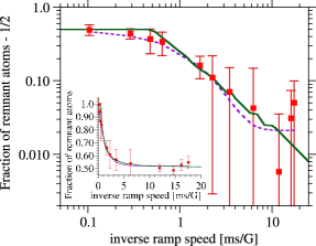
Figure 1: (Color online) Fraction of remnant atoms, $\Gamma$, versus inverse ramp speed $1/\dot{B}$ across the 543 G resonance of ⁶Li. The experimental data (red squares) of Strecker03 , which saturates at a remnant fraction of $1/2$ Pazy04 , and the mean-field calculations (solid green curve) obey a linear dependence on sweep rate beyond 0.5 ms/G. ${g^{2}\over\alpha N}$ is multiplied by 0.5 ms/G to scale the abscissa for the calculated results. Also shown as a dashed blue line in the inset is the best exponential fit to the data, $\Gamma=0.479\exp(-\alpha/1.3)+0.521$.

The paper is organized as follows. In Section II we introduce the Feshbach model-Hamiltonian and the main approximations used. In Sec. III we describe the classical phase space obtained for the above model. Section IV describes how the molecular production efficiency depends on the stability of the fixed points for the equations of motion. In Sec. V we describe the role of quantum fluctuations which lead to the linear dependence of the molecular production efficiency on the sweep rate. The analysis of sections IV and V is verified by the exact numerical calculations presented in section VI. Section VII contains summary and conclusions.

II The Zero Temperature Model System

Experiments on molecule production in slowly swept, broad Feshbach resonance systems Cubizolles03 ; Hodby are well explained by employing a thermodynamic equilibrium model Petrov . The narrow ⁶Li resonance, traversed much more rapidly Strecker03 , is not expected to fit such a description. We consider the zero temperature limit to model such experiments. At low temperatures one can use a single bosonic mode Hamiltonian Javanainen04 ; Barankov04 ; Andreev04 ; Dukelsky04 ; Tikhonenkov05 ; Miyakawa05 ; Mackie05 because of the Cooper instability which singles out the zero momentum mode of the molecules produced. Thus, we take the Hamiltonian to be

$$H = \sum_{{\bf k},\sigma}\epsilon_{\bf k}c_{{\bf k},\sigma}^{\dagger}c_{{\bf k},\sigma}+{\cal E}(t)b_{0}^{\dagger}b_{0}$$

$$+g\left(\sum_{\bf k}c_{{\bf k},\uparrow}c_{-{\bf k},\downarrow}b_{0}^{\dagger}+H.c.\right)\,,$$ (1)

where $\epsilon_{\bf k}=\hbar^{2}k^{2}/2m$ is the kinetic energy of an atom with mass $m$, and $g$ is the atom-molecule coupling strength. The molecular energy ${\cal E}(t)=E_{F}-\alpha t$ is linearly swept at a rate $\alpha>0$ where $E_{F}$ denotes the fermi energy of the atoms, through resonance to induce adiabatic conversion of fermi atoms to bose molecules. The annihilation operators for the atoms, $c_{{\bf k},\sigma}$, obey fermionic anti-commutation relations, whereas the molecule annihilation operator $b_{0}$ obeys a bosonic commutation relation.

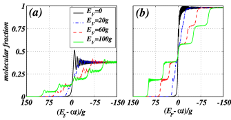
Figure 2: (Color online) Many-body collective dynamics of adiabatic passage from a fermionic atomic gas into a molecular Bose Einstein Condensate (BEC) for five pairs of fermionic atoms. (a) Sweep rate $\alpha=2g^{2}N$, (b) Sweep rate $\alpha=g^{2}N/4$. Overall efficiency is independent of atomic dispersion in both (a) and (b).

The Hamiltonian can be further simplified by neglecting fermionic dispersion. This approximation has been commonly used Mies00 ; Barankov04 and accounts for the use of a simple two-level LZ model, as opposed to a multilevel one, for such systems. To justify this assumption we have conducted many-body numerical simulations to determine the effect of fermionic dispersion on the adiabatic conversion efficiency. Fig. 2 shows exact numerical results for the adiabatic conversion of five atom pairs into molecules, for different values of the atomic level spacing (and hence of the Fermi energy $E_{F}$). It demonstrates that the final adiabatic conversion efficiency is completely insensitive to the details of the atomic dispersion. It is evident that, while the exact dynamics depends on $E_{F}$, and the levels are sequentially crossed as a function of time as the bound state crosses the level energies, the same final efficiency is reached regardless of the atomic motional timescale (i.e., regardless of level spacing). In particular, the figure shows that in the limit as $\alpha\rightarrow 0$, it is possible to convert all atom pairs into molecules. This is a unique feature of the nonlinear parametric coupling between atoms and molecules which should be contrasted with a marginal conversion efficiency expected for linear coupling in the multi-level LZ model.

Employing the degenerate model with $\epsilon_{\bf k}=\epsilon$ for all ${\bf k}$ Tikhonenkov05 ; Miyakawa05 ; Mackie05 , it is convenient to rewrite the Hamiltonian in terms of the following lowering, raising and $z$-component operators Vardi01 ; Miyakawa05 :

$${\cal J}_{-}=\frac{b_{0}^{\dagger}\sum_{{\bf k}}c_{{\bf k},\uparrow}c_{-{\bf k},\downarrow}}{(N/2)^{3/2}}~{},~{}{\cal J}_{+}=\frac{\sum_{{\bf k}}c_{-{\bf k},\downarrow}^{\dagger}c_{{\bf k},\uparrow}^{\dagger}b_{0}}{(N/2)^{3/2}}\,,$$

$${\cal J}_{z}=\frac{\sum_{{\bf k},\sigma}c_{{\bf k},\sigma}^{\dagger}c_{{\bf k},\sigma}-2b_{0}^{\dagger}b_{0}}{N}\,,$$ (2)

where $N=2b_{0}^{\dagger}b_{0}+\sum_{{\bf k},\sigma}c_{{\bf k},\sigma}^{\dagger}c_{{\bf k},\sigma}$ is the conserved total number of particles. It is important to note that ${\cal J}_{-},{\cal J}_{+},{\cal J}_{z}$ do not span $SU(2)$, since the commutator $[{\cal J}_{+},{\cal J}_{-}]$ yields a quadratic polynomial in ${\cal J}_{z}$ (despite the fact that the commutators $[{\cal J}_{+},{\cal J}_{z}]$ and $[{\cal J}_{-},{\cal J}_{z}]$ have the right commutation relations). The operators ${\cal J}_{x}={\cal J}_{+}+{\cal J}_{-}$ and ${\cal J}_{y}=-i({\cal J}_{+}-{\cal J}_{-})$ can also be defined. Up to a $c$-number term, Hamiltonian (1) takes the form

$$H=\frac{N}{2}\left(\Delta(t){\cal J}_{z}+g{\frac{\sqrt{N}}{2}}{\cal J}_{x}\right)\,,$$ (3)

where $\Delta(t)=2\epsilon-{\cal E}(t)=\alpha t$. Defining a rescaled time $\tau=\sqrt{N}gt$, and assuming a filled Fermi sea (i.e., that the number of avialable fermionic states is equal to the number of particles), we obtain the Heisenberg equations of motion,

$$\frac{d}{d\tau}{\cal J}_{x} = \delta(\tau){\cal J}_{y}\,,$$

$$\frac{d}{d\tau}{\cal J}_{y} = -\delta(\tau){\cal J}_{x}+\frac{3\sqrt{2}}{4}\left({\cal J}_{z}-1\right)\left({\cal J}_{z}+\frac{1}{3}\right)$$

$$-{\sqrt{2}\over{N}}\left(1+{\cal J}_{z}\right)\,,$$

$$\frac{d}{d\tau}{\cal J}_{z} = \sqrt{2}{\cal J}_{y}\,,$$ (4)

which depend only on the scaled detuning $\delta(\tau)=\Delta(t)/\sqrt{N}g=(\alpha/g^{2}N)\tau$. It is interesting to note that exactly these equations of motion are obtained for the two-mode atom-molecule BEC Vardi01 where, for the bosonic case, lowering, raising and $z$-component operators are defined as

$${\cal J}_{-}=\frac{b_{0}^{\dagger}a_{1}a_{2}}{(N/2)^{3/2}}~{},~{}{\cal J}_{+}=\frac{a_{2}^{\dagger}a_{1}^{\dagger}b_{0}}{(N/2)^{3/2}}\,,$$

$${\cal J}_{z}=\frac{2b_{0}^{\dagger}b_{0}-\sum_{{\bf k},\sigma}a_{{\bf k},\sigma}^{\dagger}a_{{\bf k},\sigma}}{N}\,,$$ (5)

where $a_{1}$ and $a_{2}$ are bosonic annihilation operators obeying bosonic commutation relations. In these definitions, the sign of the operator ${\cal J}_{z}$ has been reversed relative to Eq. (2), mapping fermionic association to bosonic dissociation Tikhonenkov05 ; Miyakawa05 ; Mackie05 .

III Classical phase space

The mean-field limit of Eqs. (4) is given by replacing ${\cal J}_{x},{\cal J}_{y}$, and ${\cal J}_{z}$ by their expectation values $u$, $v$, and $w$ which correspond to the real and imaginary parts of the atom-molecule coherence and the atom-molecule population imbalance, respectively. Since quantum fluctuations in ${\cal J}_{z}$ are of order $1/N$, it is also consistent to omit the quantum noise term $\sqrt{2}(1+{\cal J}_{z})/N$ in the equation for $d{\cal J}_{y}/d\tau$ in (4), as long as ${\cal J}_{z}$ is of order unity. For small $w$ however, when the molecular population is of the order of its quantum fluctuations, this quantum term becomes dominant and will have a significant effect on sweep efficiency, as will be shown in Sec. V.

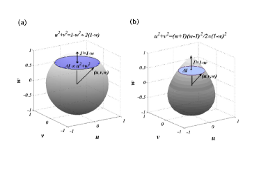
Figure 3: (Color online) Two dimensional surfaces depicting classical phase space: (a) Bloch sphere of a two-mode Bose-Josephson system, as in Refs. Vardi01 ; Liu02 (b) zero single-particle entropy surface of the atom-molecule system, as in Eqs. (6).

In the classical field limit, the equations of motion

$$\frac{d}{d\tau}u = \delta(\tau)v\,,$$

$$\frac{d}{d\tau}v = -\delta(\tau)u+\frac{3\sqrt{2}}{4}\left(w-1\right)\left(w+\frac{1}{3}\right)\,,$$

$$\frac{d}{d\tau}w = \sqrt{2}v\,,$$ (6)

depict the motion of a generalized Bloch vector on a two-dimensional ‘tear-drop’ shaped surface, (Fig. 3b), determined by the constraint,

$$u^{2}+v^{2}={1\over 2}(w-1)^{2}(w+1),$$ (7)

corresponding to the conservation of single-pair atom-molecule coherence. The peculiar shape of this equal-single-pair-entropy surface is a result of the commutation relations for the operators ${\cal J}_{-},{\cal J}_{+},{\cal J}_{z}$. For comparison, the two-level spin Hamiltonian may be written only in terms of $SU(2)$ generators Vardi01 ; Liu02 and the mean-field motion is restricted to the surface of a Bloch sphere (see Fig. 3a) as the mean-field approximation allows for the factorization of the $SU(2)$ Casimir operator ${\bf J}^{2}=J_{z}(J_{z}-1)+J_{+}J_{-}=j(j+1)$ into the constraint

$$u^{2}+v^{2}+w^{2}=j^{2}\,.$$ (8)

The surface defined by the constraint (7) should be viewed as the atom-molecule equivalent of this Bloch sphere. Accordingly, we proceed by following the methods of Ref. Liu02 which correspond to a Bloch sphere like phase space, generalizing them to the atom-molecule parametric coupling case.

Since the constraint of Eq. (7) restricts the dynamics to the two dimensional surface depicted in Fig. 3b, it is readily seen that in the mean field limit, Hamiltonian (3) is replaced by the classical form

$$H(w,\theta;\delta)=\frac{gN^{3/2}}{2}\left(\delta w+\sqrt{(1+w)(1-w^{2})}\cos\theta\right)\,.$$ (9)

Here the Hamiltonian is expressed only in terms of the relative phase between atoms and molecules $\theta\equiv\arctan(v/u)$, corresponding to the azimuthal angle in Fig. 3b, and the atom-molecule population difference $w$, corresponding to its cylindrical axial coordinate.

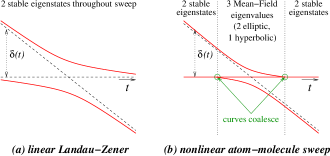
Figure 4: (Color online) The adiabatic eigenvalues of a linear LZ problem (a) are contrasted with the adiabatic level scheme of the atom-molecule nonlinear system (b). For a critical detuning, one of the adiabatic eigenvalues in (b) splits into two, resulting in the emergence of an additional hyperbolic fixed point.

The eigenvalues of the atom-molecule system at any given value of $\delta$ correspond to the extrema $(w_{0},\theta_{0})$ of the classical Hamiltonian (9), or equivalently, to the fixed points $(u_{0},v_{0},w_{0})$ of the mean-field equations (6)]:

$$v_{0}=0~{},~{}\frac{\sqrt{2}}{4}\left(w_{0}-1\right)\left(3w_{0}+1\right)=\delta u_{0}\,.$$ (10)

The number of fixed points depends on the parameter $\delta$. The point $u_{0}=v_{0}=0,w_{0}=1$ is stationary for any value of $\delta$. Using Eqs. (7) and (10), other fixed points are found from the solutions of

$$\frac{(3w_{0}+1)^{2}}{4(w_{0}+1)}=\delta^{2}\,,$$ (11)

in the domain $w_{0}\in[-1,1]$. Consequently, it is evident that for $|\delta|\geq\sqrt{2}$ there are only two stationary solutions, one of which is $w_{0}=1$. However, this stationary point bifurcates at the critical detuning of $\delta_{c}=\sqrt{2}$, so that for $|\delta|<\delta_{c}$, there are three eigenstates, as depicted in Fig. 4b. In contrast, in the linear LZ problem (Fig. 4a), eigenvalue crossings are avoided, and there are only two eigenstates throughout.

The relation between the reduced sigle-particle picture of Fig. 4b and the full many-body sytem it approximately represents, is illustrated in Fig. 5, depicting numerically calculated eigenvalues for ten atom pairs as a function of $\delta$, when $E_{F}=0$. One can envisage how, when adding more and more energy levels, finally collapsing the levels to a single curve, the curve structure of Fig. 4 emerges. The bifurcation of the all-atoms mode is shown to emerge from its quasi-degeneracy with slightly higher many-body states with a few more molecules.

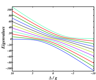
Figure 5: (Color online) The ten lowest energy eigenvalues for Hamiltonian (1), drawn for the degenerate case, $\epsilon_{\bf k}=0$.

Stability analysis of the various fixed points, preformed by linearization of the dynamical equations (4) about $(u_{0},v_{0},w_{0})$, yields the frequency $\Omega_{0}$ of small periodic orbits around them:

$$\frac{\Omega_{0}}{g\sqrt{N}}=\sqrt{\delta^{2}+(1-3w_{0})}\,.$$ (12)

From Eq. (12) it is clear that the characteristic oscillation frequency about the stationary point $(0,0,1)$ will be $\sqrt{\delta^{2}-2}$. Thus, for $\delta\geq\delta_{c}$ the point $u_{0}=v_{0}=0,w_{0}=1$ is an elliptical fixed point, whereas for $\delta\leq\delta_{c}$ it becomes a hyperbolic (unstable) stationary point, with an immaginary perturbation frequency. For the remaining eigenvalues, we can use (11) to obtain

$$\frac{\Omega_{0}}{g\sqrt{N}}=\sqrt{\frac{(1-w_{0})(3w_{0}+5)}{4(w_{0}+1)}}\,,$$ (13)

giving real $\Omega_{0}$ for all $w_{0}\in[-1,1]$, approaching zero as $w_{o}\rightarrow 1$. Consequently, for $|\delta|\leq\delta_{c}$ there are a total of two elliptical fixed points, whereas for $|\delta|<\delta_{c}$ there are two elliptical and one hyperbolic fixed points.

The fixed point analysis carried out so far is summarized in Fig. 6 where we plot the phase-space trajectories, corresponding to equal-energy contours of Hamiltonian (9), for different values of $\delta$. As expected from (9), the plots have the symmetry $(w,\theta;\delta)\leftrightarrow(w,\theta+\pi;-\delta)$. For sufficiently large detuning, $|\delta|>\sqrt{2}$, Eq. (11) has only one solution in the range $-1\leq w_{0}\leq 1$. Therefore there are two (elliptic) fixed points, denoted by a red circle corresponding to the solution of Eq. (11), and a blue square at (0,0,1). As the detuning is changed, one of these fixed points (red circle) smoothly moves from all-molecules towards the atomic mode. At the critical detuning $\delta=-\sqrt{2}$ a homoclinic orbit appears through the point $(0,0,1)$ which bifurcates into an unstable (hyperbolic) fixed point (black star) remaining on the atomic mode, and an elliptic fixed point (blue square) which starts moving towards the molecular mode. Consequently, in the regime $|\delta|<\sqrt{2}$ there are two elliptic fixed points and one hyperbolic fixed point, corresponding to the unstable all-atoms mode. Another crossing occurs at $\delta=\sqrt{2}$ when the fixed point which started near the molecular mode (red circle) coalesces with the all-atoms mode (black star). Plotting the energies of the fixed points as a function of detuning, one obtains the adiabatic level scheme of Fig. 4b.

As previously noted, for $|\delta|<\sqrt{2}$ the period of the homoclinic trajectory beginning at $(0,0,1)$ diverges. This divergence significantly affects the efficiency of an adiabatic sweep through resonance because the linear response time to a perturbation in the Hamiltonian becomes infinitely long. Consequently, the sweep is never truly adiabatic, and its expected efficiency is lower than the corresponding LZ efficiency. This effect is discussed in the following section.

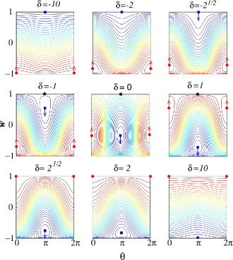
Figure 6: (Color online) Equal-energy contours of Hamiltonian (9) plotted as a function of $w$ and $\theta$ for different detunings $\delta$. $w=1$ is all atoms and $w=-1$ is all molecules. The various fixed points corresponding to adiabatic eigenvectors are marked by (blue) squares, (red) circles and (black) stars.

IV Effect of fixed-point instability on adiabatic sweep efficiency

Having characterized the classical phase-space structure for the parametrically coupled atom-molecule system, we turn to the process of adiabatically sweeping the detuning $\delta$ through resonance, converting fermion atoms into bose molecules. As usual, adiabatic following involves two typical timescales: the sweep time scale given by the inverse sweep rate $1/\alpha$ and the timescale associated with the period $1/\Omega_{0}$ of small periodic orbits around the fixed point, given in Eqs. (12) and (13). Slow changes to the Hamiltonian (e.g., by variation of the detuning $\delta$) shift the adiabatic eigenvalues, as depicted in Fig. 6. Starting with such an eigenvalue (e.g., the all-atoms mode for an initial large negative $\delta$), the state of the system will only be able to adiabatically follow the fixed point if its precession frequency about it, $\Omega_{0}$, is large compared to the rate at which it moves. The adiabatic conversion efficiency is related to the magnitude of this precession, which in turn is proportonal to the classical action accumulated during the sweep.

The relation between the sweep conversion efficiency and the accumulated classical action is illustrated in Fig. 3. Consider first the $SU(2)$ case of Fig. 3a, where mean-field motion is restricted to the surface of the Bloch sphere $u^{2}+v^{2}+w^{2}=1$. This illustration applies to the standard LZ case Landau as well as to the nonlinear Bose-Josephson system Vardi01 ; Liu02 ; Garraway00 . Having started from the ‘south pole’ $(0,0,-1)$ and carried out the sweep through resonance, the classical state Bloch vector $(u,v,w)$ carries out small precessions about the final adiabatic eigenvector which (for sufficiently large final detuning) is parallel to the $w$ axis. The surface-area enclosed within this periodic trajectory is just the action, $\Delta I\propto u^{2}+v^{2}$, accumulated during the sweep. In the extreme limit of perfect adiabatic following, the precession approaches a point trajectory, having zero action. Larger nonadiabaticity leads to larger precession amplitude, and hence to larger accumulated action. The remanent fraction in the initial state, $\Gamma=(1-w)$, is directly related to $\Delta I$ by the conservation rule $u^{2}+v^{2}=(1+w)(1-w)$, which near $w=1$ can be linearized to give $\Delta I\approx 2\Gamma$. This is the expression usually used in calculating LZ transition probabilities Landau ; Liu02 .

For the atom-molecule parametric system of Fig. 3b, the situation is slightly different, since $u^{2}+v^{2}=(1+w)(1-w)^{2}$, leading to a square root dependence of the remnent atomic fraction $\Gamma$ on $\Delta I$ near $w=1$. In order to estimate $\Delta I$, we transform $w,\theta$ into action-angle variables $I,\phi$. In terms of these variables the non-adiabatic probability $\Gamma$ at any finite sweep rate $\alpha$ is given by

$$\Gamma^{2}=\frac{\Delta I}{2}={1\over 2}\int_{-\infty}^{\infty}R(I,\phi)\,{\dot{\Delta}}\,\frac{d\phi}{{\dot{\phi}}}\,,$$ (14)

where $R(I,\phi)$ is related to the generating function of the canonical transformation $(w,\theta)\rightarrow(I,\phi)$ Landau_L ; Liu02 .

Equation (14) reflects our discussion on characteristic timescales. In order to attain adiabaticity, the rate of change of the adiabatic fixed points through the variation of the adiabatic parameter $\Delta$, $R(I,\phi)\,{\dot{\Delta}}$, should be slow with respect to the characteristic precession frequency ${\dot{\phi}}=\Omega_{0}$ about these stationary vectors. The action increament is proportional to the ratio of these two timescales.

As long as ${\dot{\phi}}$ does not vanish, the accumulated action can be minimized by decreasing ${\dot{\Delta}}$. For a perfectly adiabatic process where ${\dot{\Delta}}/{\dot{\phi}}\rightarrow 0$, the action is an adiabatic invariant, so that a zero-action elliptic fixed point evolves into a similar point trajectory. For finite sweep rate, the LZ prescription Landau evaluates the integral in (14) by integration in the complex plain, over the contour of Fig. 7, noting that the main contributions will come from singular points, where ${\dot{\phi}}$ approaches zero and the integrand diverges. Since for a linear LZ system there are no instabilities, all such singularities are guarenteed to lie off the real axis, leading to the exponentially small LZ transition probabilities.

The situation changes for nonlinear systems, where instabilities arrise. In section III we have shown that for the atom-molecule system with fermion atoms, the all-atoms mode becomes unstable to association when the detuning hits the critical value of $\delta_{c}=\sqrt{2}$. From Eq. (12) it is clear that the characteristic frequency ${\dot{\phi}}=\Omega_{0}$ vanishes near $w_{0}=0$. Consequently, there are singular points of the integrand in (14) lying on the real axis. In what follows, we show that these poles on the real axis lead to power-law dependence of the transfer efficiency on the sweep rate.

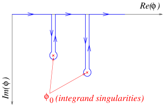
Figure 7: (Color online) Contour of integration in LZ theory, for calculating the integral in Eq. (14). All singularities lie off the real axis.

In order to evaluate the integral (14), we need to investigate how the characteristic frequency ${\dot{\phi}}=\Omega_{0}$ depends on the action-angle $\phi$ near the instability point $(u=0,v=0,w=1)$, where most action (and hence most nonadiabatic correction) is accumulated. It is evident from Eq. (12) that the precession frequency near that point vanishes as

$$\Omega_{0}\approx g\sqrt{N(1-w_{0})}\,.$$ (15)

Differentiating Eq. (11) with respect to $t$, we find that the rate of change of adiabatic fixed-points due to a linear sweep is,

$${{\dot{w}}_{0}}=\frac{4\alpha}{g\sqrt{N}}\frac{(w_{0}+1)^{3/2}}{3w_{0}+5}\,.$$ (16)

Having found ${{\dot{w}}_{0}}$, we can now find the explicit form of the transformation from $w_{0}$ to the action-angle variable $\phi$, near the instability. The action-angle may be written as

$$\phi=\int{\dot{\phi}}dt=\int\Omega_{0}\frac{dw_{0}}{{\dot{w}}_{0}}\,.$$ (17)

In the vicinity of the singularity ($w_{0}=1$) we have $\Omega_{0}\approx g\sqrt{N(1-w_{0})}$ and ${\dot{w}}_{0}\approx{\sqrt{2}\alpha/g\sqrt{N}}$, resulting in

$$\phi=\frac{g^{2}N}{\alpha}\frac{\sqrt{2}}{3}(1-w_{0})^{3/2}\,.$$ (18)

Thus, as the adiabatic eigenstate approaches $w_{0}=1$ the angle $\phi$ vanishes as $(1-w_{0})^{3/2}$ whereas the characteristic frequency ${\dot{\phi}}$ approaches zero as $(1-w_{0})^{1/2}$. Consequently, we finally find from (15) and (18) that near the singularity, $\dot{\phi}$ is given in terms of $\phi$ as

$${\dot{\phi}}=\left(3\sqrt{N\over 2}g\alpha\right)^{1/3}\phi^{1/3}\,.$$ (19)

Substituting (19) and $\dot{\Delta}=\alpha$ into Eq. (14) we find that the nonadiabatic correction depends on $\alpha$ as

$$\Gamma\propto\alpha^{1/3}\,.$$ (20)

V Quantum Fluctuations

So far, we have neglected the effect of quantum fluctuations, which may be partially accounted for by the $c$-number limit of the source term $(\sqrt{2}/N)(1+{\cal J}_{z})$ in Eqs. (4). As a result, we found in the previous section that $\dot{w}_{0}$ does not vanish as $w_{0}$ approaches unity, and the remaining atomic population scales as the cubic root of the sweep rate if the initial average molecular fraction is larger than the quantum noise. However, starting purely with fermion atoms (or with molecules made of bosonic atoms), corresponding to an unstable fixed point of the classical phase space, fluctuations will serve to trigger the association process and will thus initially dominate the conversion dynamics.

In order to verify that such quantum fluctuations can be accurately reproduced by a ‘classical’ noise term near the unstable fixed point $w=1$, we compare the onset of instability from exact many-body calculations to the onset of mean-field instability according to the revised mean-field equations,

$$\frac{d}{d\tau}u = \delta(\tau)v\,,$$

$$\frac{d}{d\tau}v = -\delta(\tau)u+\frac{3\sqrt{2}}{4}\left(w-1\right)\left(w+\frac{1}{3}\right)$$

$$+\frac{\sqrt{2}}{N}(1+w)\,,$$

$$\frac{d}{d\tau}w = \sqrt{2}v\,,$$ (21)

where we have retained the ${\cal O}(1/N)$ noise term $(\sqrt{2}/N)(1+w)$. The results, shown in Fig. 8, show excellent agreement in the early-time dynamics, indicating that the mean-field noise term gives the correct behavior near the instability point.

Having established the accuracy of the noise term in Eqs. (21) we proceed to investigate its effect on sweep efficiencies. When this additional term is accounted for, Eq. (11) must be replaced by

$$\delta=\frac{2}{\sqrt{w_{0}+1}}\left(\frac{3w_{0}+1}{4}-\frac{w_{0}+1}{N(w_{0}-1)}\right)\,.$$ (22)

This expression reduces to our previous result in Eq. (11) when the second term on the r.h.s. of Eq. (22), resulting from the quantum fluctuations, can be neglected compared to the first term. Since $\frac{3w_{0}+1}{4}$ is of order unity around $w_{0}=1$, our previous treatment is only valid provided that $|w_{0}(t_{i})-1|\gg 1/N$.

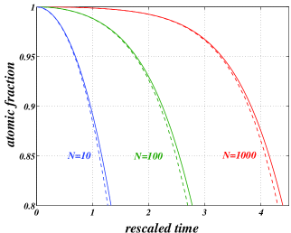
Figure 8: (Color online) Atomic population fraction versus time, starting with a gas of fermion atoms using exact $N=10,100,1000$ particle calculations (solid lines) and the mean-field theory of Eqs. (21) (dashed lines), with $\delta=0$.

For smaller initial molecular population, Eq. (16) should be replaced by

$${{\dot{w}}_{0}}=\frac{\alpha}{g\sqrt{N}}\left/\left[\frac{3w_{0}+5}{4(w_{0}+1)^{3/2}}+\frac{w_{0}+3}{N(w_{0}+1)^{1/2}(w_{0}-1)^{2}}\right]\right..$$ (23)

Hence, in the vicinity of $w_{0}=1$ the eigenvector velocity in the $w$ direction vanishes as

$${{\dot{w}}_{0}}=(\sqrt{N}\alpha/g\sqrt{8})\left(w_{0}-1\right)^{2}\,.$$ (24)

In contrast to the nonvanishing eigenvalue velocity in Eq. (16). Substituting ${\dot{w}}_{0}$ from Eq. (24) into Eq. (17), we obtain the action-angle,

$$\phi=-\frac{\sqrt{32}g^{2}}{\alpha}(w_{0}-1)^{-1/2}\,.$$ (25)

The characteristic frequency $\dot{\phi}$ is now proportional to $(\alpha\phi)^{-1}$ instead of Eq. (19) so that $\Delta I\propto\alpha^{2}$, and Ishkhanyan04 ; Altman05 ; Barankov05

$$\Gamma\propto\alpha~{}.$$ (26)

Equations (26) and (20) constitute the main results of this work. We predict that the remnant atomic fraction in adiabatic Feshbach sweep experiments scales as a power-law with sweep rate due to the curve crossing in the nonlinear case. When the system is allowed to go near the critical point (i.e., when $1-w_{0}(t_{i})\ll 1/N$) quantum fluctuations are the major source of non-adiabtic corrections, leading to a linear dependence of the remnent atomic fraction on the sweep rate. We note that a similar linear dependence was predicted for adiabatic passage from bosonic atoms into a molecular BEC Ishkhanyan04 . When the initial state is such that it has already a large molecular population (i.e. for $1-w_{0}(t_{i})\gg 1/N$) and fluctuations can be neglected, we obtain a cubic-root dependence of the the final atomic fraction on sweep rate.

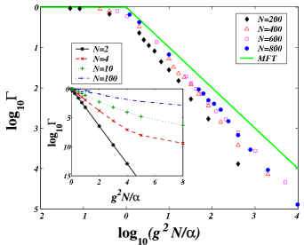
Figure 9: (Color online) Many-body calculations for the fraction of remnant atoms, $\Gamma$, versus dimensionless inverse sweep rate for various particle numbers in the range $N=2$ to 800. The many-body results for large number of particles converge to the mean-field results (solid green line) computed numerically from the mean-field limit of Eqs. (4).

VI Numerical Many-Body Results, and Comparison to Experiment

In order to confirm the predictions of Section IV and Section V, we carried out excat many-body numerical calculation for particle numbers in the range $2\leq N\leq 800$, by Fock-space representation of the operators ${\cal J}_{i}$ and direct propagation of the many-body equations (4), according to the methodology of Tikhonenkov05 . Fig. 9 shows $\Gamma$ versus dimensionless inverse sweep rate ${g^{2}N/\alpha}$. The exact calculations are compared with a mean-field curve (solid green line), computed numerically from the mean-field equations (21). The log-log plot highlights the mean-field power-law dependence, obtained in the slow ramp regime $\alpha<g^{2}N$, whereas the log-linear insert plot demonstrates exponential behavior. For a single pair of particles, $N=2$, the quantum association problem is formally identical to the linear LZ paradigm, leading to an exponential dependence of $\Gamma$ on sweep rate (see insert of Fig. 1). However, as the number of particles increases, many-body effects come into play, and there is a smooth transition to a power-law behavior in the slow ramp regime $\alpha<g^{2}N$. We note that this is precisely the regime where Eq. (14) can be used to estimate $\Delta I$ and $\Gamma$ Landau . The many-body calculations converge to the mean-field limit, corresponding to a linear dependence of $\Gamma$ on $\alpha$, as predicted in Eq. (26).

The results shown in Fig. 9 prove the convergence of many-body calculations to the mean-field theory used as a basis to our analysis in previous sections. Having established the validity of this classical field theory, and numerically confirmed the appearance of power-law behavior, we return to the experimental results of Ref. Strecker03 shown in Fig. 1. Comparison of our mean-field numerical calculation with the experimental data (red squares in Fig. 1) clearly shows good agreement. However, since an equally good exponential fit can be found Strecker03 , as shown in the insert of Fig. 1 (dashed line), current experimental data does not serve to determine which of the alternative theories is more appropriate. We have obtained similar agreement with the experimental data of Ref. Regal03 , but data scatter and error bars are again too large to conclusively resolve power-laws from exponentials. Additional precise experimental data over a wider range of slow ramp sweep rates and different particle numbers will be required to verify or to refute our theory.

VII Summary and Discussion

We have shown that nonlinear effects can play a significant role in the atom-molecule conversion process for degenerate fermionic atomic gases. In linear LZ theory, the precession of the two-state Bloch vector about the adiabatic eigenstate never stops (all the poles of the the integrand in Eq. (14) lie off the real axis), leading to exponential dependence on sweep rate. The nonlinear nature of the reduced mean-field dynamics in the large $N$ limit of the many-body system, introduces dynamical instabilities. For the fermionic association case, it is the all-atoms mode that becomes unstable. The period of the precession about this mode diverges, leading to real singularities of the integrand in (14). Consequently, power-law nonadiabaticity is obtained.

While the experimental data was originally fit with LZ exponential behavior Strecker03 , it fits a power-law dependence just as well. Future experimental work with a larger range of sweep rates, should serve to determine which fit is best at low temperatures.

The modification of LZ behavior into a $\Gamma\propto\alpha^{3/4}$ power-law dependence, has been predicted for linearly-coupled, interacting Bose-Josephson systems Liu02 ; Garraway00 . Here, and in Ref. Pazy05 , we applied the theoretical technique of Liu02 , adapting it to the case of a non-spherical two dimensional phase space surface. The exact power-law for the atom-molecule system was shown to depend on the role quantum noise plays in the conversion process. When it is negligible, we find that $\Gamma\propto\alpha^{1/3}$. However, starting from a purely atomic gas, quantum fluctuations dominate the dynamics, resulting in a $\Gamma\propto\alpha$ power law. The same linear dependence was previously found for the bosonic photoassociation problem Ishkhanyan04 .

Our numerical results support our analytical predictions, demonstrating how exponential LZ behavior, applicable to two atoms, is transformed into a power law dependence as the number of atoms increases (see Fig. 9). The analysis based on Eq. (14) makes the differences between the two cases transparent, relating them to different types of singularities.

We note that the same power laws of $\Gamma\propto\alpha^{1/3}$ and $\Gamma\propto\alpha$ appear in recent theoretical studies of dynamical projection onto Feshbach molecules Altman05 ; Barankov05 . The power-law in Altman05 results from the nature of the projected pairs, correlated pairs giving a $\Gamma\propto\alpha^{1/3}$ power law whereas uncorrelated pairs give linear dependence, due to their respective overlaps with the molecular state. For comparison, the quantum noise term in our analysis corresponds to initial uncorrelated spontaneous emission, leading to $\Gamma\propto\alpha$ linear behavior, whereas for a larger initial molecular population, correlations between emitted pairs are established and emission becomes coherent, yielding the $\Gamma\propto\alpha^{1/3}$ power law. The approach taken in Barankov05 is rather different, based on a variant of the Wiener-Hopf method, yet it results in precisely the same power-laws.

- (1) W. C. Stwalley, Phys. Rev. Lett. 37, 1628 (1976).
- (2) E. Tiesinga et al., Phys. Rev. A 47, 4114 (1993).
- (3) S. Inouye, M. R. Andrews, J. Stenger, H.-J. Miesner, D. M. Staper-Kurn, and W. Ketterle, Nature 392, 151 (1998).
- (4) F. H. Mies et al., Phys. Rev. A61, 022721 (2000); K. Góral et al., J. Phys. B37, 3457 (2004); J. Chwedeńczuk et al., Phys. Rev. Lett. 93, 260403 (2004).
- (5) E. Timmermans, P. Tommasini, M. Hussein, and A. Kerman, Phys. Rep. 315, 199 (1999).
- (6) C. A. Regal, C. Ticknor, J. L. Bohn, and D. S. Jin, Nature (London) 424, 47 (2003).
- (7) K. E. Strecker, G. B. Partridge, and R. G. Hulet, Phys. Rev. Lett. 91, 080406 (2003).
- (8) J. Cubizolles, T. Bourdel, S.J.J.M.F. Kokkelmans, G.V. Shlyapnikov, and C. Salomon, Phys. Rev. Lett. 91, 240401 (2003).
- (9) E. Hodby et al., Phys. Rev. Lett. 94, 120402 (2005).
- (10) M. Greiner et al., Nature (London) 426, 537 (2003).
- (11) S. Jochim et al., Science 302, 2101 (2003).
- (12) M.W. Zwierlein et al., Phys. Rev. Lett. 91, 250401 (2003).
- (13) N. R. Claussen, E. A. Donley, S. T. Thompson, and C. E. Wieman, Phys. Rev. Lett. 89, 010401 (2002).
- (14) J. Herbig, T. Kraemer, M. Mark, T. Weber, C. Chin, H.-C. Nägerl, and R. Grimm, Science 301, 1510 (2003).
- (15) S. Durr et al., Phys. Rev. Lett. 92, 020406 (2004). S. Durr, T. Volz, A. Marte, and G. Rempe, Phys. Rev. Lett. 92, 020406 (2004).
- (16) D.S. Petrov, C. Salomon, and G.V. Shlyapnikov Phys. Rev. Lett. 93, 090404 (2004).
- (17) E. Pazy, I. Tikhonenkov, Y. B. Band, M. Fleischhauer, and A. Vardi Phys. Rev. Lett. 95, 170403 (2005).
- (18) L. D. Landau, Phys. Z. Sowjetunion 2, 46 (1932); G. Zener, Proc. R. Soc. London, Ser. A137, 696 (1932).
- (19) E. Pazy, A. Vardi and Y. B. Band, Phys. Rev. Lett. 93, 120409 (2004).
- (20) J. Javanainen et al., Phys. Rev. Lett. 92, 200402 (2004).
- (21) R. A. Barankov and L. S. Levitov, Phys. Rev. Lett. 93, 130403 (2004).
- (22) A. V. Andreev et al., Phys. Rev. Lett. 93, 130402 (2004).
- (23) J. Dukelsky, G. G. Dussel, C. Esebbag, and S. Pittel, Phys. Rev. Lett. 93, 050403 (2004).
- (24) I. Tikhonenkov and A. Vardi, cond-mat/0407424.
- (25) T. Miyakawa and P. Meystre, Phys. Rev. A71, 033624 (2005).
- (26) M. Mackie and O. Dannenberg, physics/0412048.
- (27) A. Vardi, V. A. Yurovsky, and J. R. Anglin, Phys. Rev. A64, 063611 (2001).
- (28) L. D. Landau and E. M. Lifshitz, Mechanics (Pergamon, Oxford, 1976), Sec. 51.
- (29) J. Liu, L. Fu, B.-Y. Ou, S.-G. Chen, D.-I. Choi, B. Wu, and Q. Niu, Phys. Rev. A 66, 023404 (2002).
- (30) O. Zobay and B. M. Garraway, Phys. Rev. A61, 033603 (2000).
- (31) A. Ishkhanyan, M. Mackie, A. Carmichael, P. L. Gould, and J. Javanainen, Phys. Rev. A 69, 043612 (2004).
- (32) E. Altman and A. Vishwanath, Phys. Rev. Lett. 95, 110404 (2005).
- (33) R. A. Barankov and L. S. Levitov, cond-mat/0506323.