Entropy-induced separation of star polymers in porous media

Abstract

We present a quantitative picture of the separation of star polymers in a solution where part of the volume is influenced by a porous medium. To this end, we study the impact of long-range-correlated quenched disorder on the entropy and scaling properties of $f$-arm star polymers in a good solvent. We assume that the disorder is correlated on the polymer length scale with a power-law decay of the pair correlation function $g(r)\sim r^{-a}$. Applying the field-theoretical renormalization group approach we show in a double expansion in $\varepsilon=4-d$ and $\delta=4-a$ that there is a range of correlation strengths $\delta$ for which the disorder changes the scaling behavior of star polymers. In a second approach we calculate for fixed space dimension $d=3$ and different values of the correlation parameter $a$ the corresponding scaling exponents $\gamma_{f}$ that govern entropic effects. We find that $\gamma_{f}-1$, the deviation of $\gamma_{f}$ from its mean field value is amplified by the disorder once we increase $\delta$ beyond a threshold. The consequences for a solution of diluted chain and star polymers of equal molecular weight inside a porous medium are: star polymers exert a higher osmotic pressure than chain polymers and in general higher branched star polymers are expelled more strongly from the correlated porous medium. Surprisingly, polymer chains will prefer a stronger correlated medium to a less or uncorrelated medium of the same density while the opposite is the case for star polymers.

I INTRODUCTION

The influence of structural disorder on the scaling properties of polymer macromolecules, dissolved in a good solvent is subject to ongoing intensive discussions Chakrabarti (2005); Barat and Chakrabarti (1995); Harris (1983); Kim (1983); Blavats’ka et al. (2001a, b); Blavats’ka et al. (2002); Kremer (1981); Meir and Harris (1989); Nakanishi and Lee (1991); Grassberger (1993); Ordemann et al. (2000); von Ferber et al. (2004). For polymers, structural disorder may be realized experimentally by a porous medium. Depending on the way the latter is prepared, it can mimic various behavior, ranging from uncorrelated defects Li and Sieradzki (1992); Gelb and Gubbins (1998); Chan et al. (1988); Yoon and Chan (1997) to complicated fractal objects Vacher et al. (1988); Pekala and Hrubesh (1995); Yoon et al. (1998). Consequently, theoretical and Monte Carlo (MC) studies have considered these different types of disorder. In particular, the scaling properties of polymer chains were analyzed for the situations of weak uncorrelated Harris (1983); Kim (1983), of long-range-correlated Blavats’ka et al. (2001a, b); Blavats’ka et al. (2002) as well as of fractal disorder at the percolation threshold Kremer (1981); Meir and Harris (1989); Nakanishi and Lee (1991); Grassberger (1993); Ordemann et al. (2000); von Ferber et al. (2004). However, as far as the authors know, the influence of correlated disordered media on the behavior of branched polymers, e.g. polymer stars, have found less attention. Our work is intended to fill this gap.

The study of star polymers is of great interest since it has a close relationship to the subject of micellar and other polymeric surfactant systems Grest et al. (1996); von Ferber and Holovatch (2002); Likos (2001). Moreover, it can be shown, that the scaling behavior of simple star polymers also determines the behavior of general polymer networks of more complicated structure Duplantier (1989); Schäfer et al. (1992). Recently, progress in the synthesis of high quality mono-disperse polymer networks Roovers and Bywater (1972); Roovers et al. (1983); Khasat et al. (1988); Bauer et al. (1989); Merkle et al. (1993) has stimulated numerous theoretical studies of star polymers, both by computer simulation Grest et al. (1987); Barrett and Tremain (1987); Batoulis and Kremer (1989); Ohno (1994); Shida et al. (1996); Hsu et al. (2004) and by the renormalization group technique Duplantier (1989); Schäfer et al. (1992); Miyake and Freed (1983); Duplantier (1986); Ohno and Binder (1988); Ohno (1989); Ohno and Binder (1991); von Ferber and Holovatch (1995, 1996); von Ferber and Holovatch (1997a, b); von Ferber and Holovatch (1999, 2002); von Ferber (2004); Schulte-Frohlinde et al. (2004). Let us note, that polymer stars are hybrids between polymer like entities and colloidal particles, establishing an important link between these different systems Grest et al. (1996); von Ferber and Holovatch (2002); Likos (2001); Likos et al. (1998); Watzlawek et al. (1999); Jusufi et al. (1999).

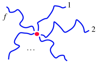
Figure 1: Polymer star with $f$ arms.

It is well established that long flexible polymer chains in good solvents display universal and self-similar conformational properties on a coarse-grained scale and that these are perfectly described within a model of self-avoiding walks (SAWs) on a regular lattice des Cloizeaux and Jannink (1990); Schäfer (1999); de Gennes (1979). For the average square end-to-end distance $R$ and the number of configurations $Z_{N}$ of a SAW of $N$ steps one finds in the asymptotic limit $N\to\infty$:

$$\langle R^{2}\rangle\sim N^{2\nu},\mbox{\hskip 30.00005pt}Z_{N}\sim{\rm e}^{\mu N}N^{\gamma-1}$$ (1)

where $\nu$ and $\gamma$ are the universal exponents depending only on the space dimensionality $d$, and ${\rm e}^{\mu}$ is a non-universal fugacity. The universal properties of this polymer model can be described quantitatively with high precision by analyzing a corresponding field theory by renormalization group methods des Cloizeaux and Jannink (1990); Schäfer (1999); Brezin et al. (1976); Zinn-Justin (1996); Kleinert and Schulte-Frohlinde (2001); Amit (2.ed.1984). For $d=3$ the exponents read Guida and Zinn-Justin (1998) $\nu^{(0)}=0.5882\pm 0.0011$ and $\gamma^{(0)}=1.1596\pm 0.0020$. Here, and in the following we use the notation $x^{(0)}$ for the value of an exponent derived for the pure solution without disorder.

The power laws of Eq. (1) can be generalized to describe a star polymer that consists of $f$ linear polymer chains or SAWs, linked together at their end-points (see Fig. 1). For a single star with $f$ arms of $N$ steps (monomers) each, the number of possible configurations scales according to Duplantier (1989); Schäfer et al. (1992):

$$Z_{N,f}\sim{\rm e}^{\mu Nf}N^{\gamma_{f}-1}\sim(R/\ell)^{\eta_{f}-f\eta_{2}}$$ (2)

in the asymptotic limit $N\to\infty$ . The second part shows the power law in terms of the size $R\sim N^{\nu}$ of the isolated chain of $N$ monomers on some microscopic step length $\ell$, omitting the fugacity factor. The exponents $\gamma_{f}$, $\eta_{f}$ are universal star exponents, depending on the number of arms $f$. The relations between these exponents read Duplantier (1989)

$$\gamma_{f} = 1+\nu(\eta_{f}-f\eta_{2})$$

$$\gamma_{1}=\gamma_{2}=\gamma = 1-\nu\eta_{2},\mbox{\hskip 20.00003pt}\eta_{1}=0.$$ (3)

Here, $\nu$ and $\gamma$ are usual SAW exponents (1). For $f=1$, $2$ the case of a single polymer chain is restored. Recent numerical values for $\gamma_{f}$ for different $f$ at $d=3$ are given in Refs. Grest et al. (1987); Barrett and Tremain (1987); Batoulis and Kremer (1989); Ohno (1994); Shida et al. (1996); Hsu et al. (2004) for Monte Carlo (MC) simulations and in Refs.Schäfer et al. (1992); Miyake and Freed (1983); Duplantier (1986); Ohno and Binder (1988); Ohno (1989); Ohno and Binder (1991); von Ferber and Holovatch (1995, 1996) for renormalization group calculations.

In terms of the mutual interaction, polymer stars interpolate between single polymer chains (low $f$) and polymeric micelles (high $f$) Likos et al. (1998); Watzlawek et al. (1999); Jusufi et al. (1999). From the scaling properties of star polymers, one may also derive their short distance effective interaction. The mean force $F(r)$ between two star polymers of $f$ and $f^{\prime}$ arms is inversely proportional to the distance $r<R$ between their cores, Duplantier (1989); von Ferber et al. (2001):

$$\frac{1}{k_{B}T}\,F(r)=\frac{\Theta_{ff^{\prime}}}{r},$$ (4)

with the amplitude given by the universal contact exponent $\Theta_{ff^{\prime}}$. The contact exponents are related to the family of exponents $\eta_{f}$ for single star polymers by the following scaling relation (2) Duplantier (1989):

$$\Theta_{ff^{\prime}}=\eta_{f}+\eta_{f^{\prime}}-\eta_{f+f^{\prime}}.$$ (5)

Figure 2: Separation phenomena of polymer stars in good solution, part of which is in a porous medium.

Similar to the model of SAWs on a regular lattice which is used to describe the scaling properties of long flexible polymer chains in a good solvent, one may consider models of SAWs on disordered lattices to study polymers in a disordered medium. In this model, a given fraction of the lattice sites is randomly chosen to be forbidden for the SAW (these forbidden sites will be called defects hereafter). Harris Harris (1983) conjectured that the presence of weak quenched uncorrelated point-like defects should not alter the SAW critical exponents. This was later confirmed by renormalization group considerations Kim (1983). Another picture appears however for strong disorder, when the fraction of allowed sites is at the percolation threshold. Numerous data from exact enumeration, analytical and MC simulation Kremer (1981); Meir and Harris (1989); Nakanishi and Lee (1991); Grassberger (1993); Ordemann et al. (2000); von Ferber et al. (2004) strongly suggest that the scaling of a SAW on a percolation cluster belongs to a new universality class and is governed by exponents, that differ from those of a SAW on a regular lattice.

Our present study concerns the scaling properties of star polymers in porous media which are found to display correlations on a mesoscopic scale Sahimi (1995). In small angle X-ray and neutron scattering experiments these correlations often express themselves by a power law behavior of the structure factor $S(q)\sim q^{-d_{f}}$ on scales $\xi^{-1}<q<\ell^{-1}$ where $\ell$ is a microscopic length scale and $\xi$ is the correlation length of the material and $d_{f}$ is its fractal volume dimension Hasmy et al. (1995). We describe this medium by a model of long-range-correlated (extended) quenched defects. This model was proposed in Ref. Weinrib and Halperin (1983) in the context of magnetic phase transitions. It considers defects, characterized by a pair correlation function $g(r)$, that decays with a distance $r$ according to a power law:

$$g(r)\sim r^{-a}$$ (6)

at large $r$. For the structure factor this leads to a power law behavior with fractal dimension $d_{f}=d-a$ where $d$ is the Euclidean space dimension. This type of disorder has a direct interpretation for integer values of $a$. Namely, the case $a=d$ corresponds to point-like defects, while $a=d-1$ $(a=d-2)$ describes straight lines (planes) of impurities of random orientation. Non-integer values of $a$ are interpreted in terms of impurities organized in fractal structures Weinrib and Halperin (1983).

The influence of the long-range-correlated defects (6) on magnetic phase transitions has been pointed out in theoretical work Weinrib and Halperin (1983); Dorogovtsev (1984); Korutcheva and de la Rubia (1998); Prudnikov and Fedorenko (1999); Prudnikov et al. (1999, 2000) and MC simulations Ballesteros and Parisi (1999); Vasquez et al. (2003); Prudnikov et al. (2005). For polymers, its impact on the scaling of single polymer chains was analyzed in our previous work in two complementary renormalization group approaches: first by a double expansion in the parameters $\varepsilon=4-d$ and the correlation strength $\delta=4-a$ using a linear approximation Blavats’ka et al. (2001a) and secondly by evaluating two-loop expressions of the theory for fixed values of $a$ and $d$ Blavats’ka et al. (2001b); Blavats’ka et al. (2002). In particular, this work showed that long-range-correlated disorder leads to a new universality class with values of the polymer scaling exponents that depend on the strength of the correlation expressed by the parameters $a$ or $\delta=4-a$. From this we may expect that also the architecture dependent scaling behavior (2) of polymer stars and networks is affected by this type of correlated disorder.

The question we are interested in is: how does the presence of long-range-correlated disorder change the values of the critical exponents (2), (4)? Besides the star-star interaction, the exponents govern various phenomena that involve star polymers and polymer networks von Ferber and Holovatch (1997a, b); von Ferber and Holovatch (1999, 2002); von Ferber (2004); Schulte-Frohlinde et al. (2004). A particular effect that may be observable experimentally for star polymer solutions in a porous medium is an architecture-dependent impact of the medium on the star polymer. It may lead to a separation of star polymers with different numbers $f$ of arms. Let us consider star polymers in a good solvent, part of which is in a porous medium (see Fig. 2). We consider the pores to be large enough, so that the star polymers may pass in and out of the medium (however, possibly on long time scales only). Be ${\cal F}^{(0)}_{f}(N)$ the free energy of a star polymer with $f$ arms of $N$ steps each in the pure solvent and ${\cal F}^{(\delta)}$ its free energy in a porous medium characterized by a correlation strength $\delta$. These can be estimated using (2):

$${\cal F}^{(0)}_{f}(N) = -\ln{\cal Z}^{(0)}_{f}(N)$$ (7)

$$=-\mu(0)Nf-(\gamma_{f}^{(0)}-1)\ln N\,,$$

$${\cal F}^{(\delta)}_{f}(N) = -\ln{\cal Z}^{(\delta)}_{f}(N)$$ (8)

$$=-\mu(\rho)Nf-(\gamma_{f}^{(\delta)}-1)\ln N\,.$$

Here, we assume the fugacity factor $e^{-\mu(\rho)}$ to depend on the concentration of impurities independent of their correlation, as it would be the case for SAWs on a lattice with corresponding defects Grassberger (1993). The product $Nf$ represents the total number of steps or effective monomers of the star polymer which is a dimensionless measure of its molecular mass. Using Eqs. (7) and (8) one may now compare the free energies of a number of situations. Let us name mainly two specific questions: (i) Given a star polymer with fixed mass $Nf$ and functionality $f$ in a good solution in a volume that is influenced by disorder with a fixed defect density $\rho$. Does the free energy depend on the correlation, and in particular is the uncorrelated disorder or rather the correlated disorder of the same density favored by the star polymer? (ii) Given a mixture of star polymers which are mono-disperse in mass $Nf$ but polydisperse in functionality $f$ in a good solution in which only a part of the volume is influenced by defects (see Fig. 2). Due to the fugacity contribution which is the same for all these star polymers, they are expected to favor the pure part of the solution. However the extent to which this is the case may depend on architecture. Is the star polymer mixture partly separated in this situation and where is the concentration of higher branched star polymers enhanced in this case? While our answer to the first question is mainly to be compared with MC simulations of star polymers on disordered lattices, the answer to the second one may also be relevant for experiments with polymers in solutions inside correlated structures like aerogels.

The setup of the paper is as follows. In the next section we present the model and construct the Lagrangean of the corresponding field theory. In section III we describe the field-theoretical renormalization group (RG) methods that we apply. Section IV presents our results for the two RG approaches. We conclude with an interpretation of these results in section V.

II THE MODEL

Let us consider a single star polymer with $f$ arms immersed in a good solvent (Fig. 1). Working within the Edwards continuous chain model Edwards (1965, 1966), we represent each arm of the star by a path ${\bf r}_{\alpha}(s)$, parameterized by $0\leq s\leq S$, $\alpha=1,2,\ldots,f$. In a corresponding discrete model of chains with $N$ steps of mean square microscopic length $\ell$ the so-called Gaussian surface is $S=N\ell^{2}$. The central branching point of the star is fixed at ${\bf r}_{1}(0)$. The partition function of the system is then defined by the functional integral Schäfer et al. (1992):

$${\cal Z}_{f}(S) = \int D[{\bf r}_{1},\ldots,{\bf r}_{f}]$$ (9)

$$\times\exp\left[-{\cal H}_{f}\right]\prod_{\alpha=2}^{f}\delta^{d}({\bf r}_{\alpha}(0)-{\bf r}_{1}(0)).$$

Here, ${\cal H}_{f}$ is the Hamiltonian, describing the system of $f$ disconnected polymer chains:

$${\cal H}_{f} = \frac{1}{2}\sum_{\alpha=1}^{f}\int_{0}^{S}{\rm d}\,s\left(\frac{{\rm d}\,{\bf r}_{\alpha}(s)}{{\rm d}s}\right)^{2}$$

$$+\frac{u_{0}}{4!}\sum_{\alpha,\alpha^{\prime}=1}^{f}\int_{0}^{S}{\rm d}s\int_{0}^{S}{\rm d}s^{\prime}\delta^{d}({\bf r}_{\alpha}(s)-{\bf r}_{\alpha^{\prime}}(s^{\prime})).$$

The first term in (II) represents the chain connectivity whereas the second term describes the short range excluded volume interaction. The product of $\delta$-functions in (9) ensures the star-like configuration of the set of $f$ chains requiring each of them to start at the point ${\bf r}_{1}(0)$. This model may be mapped to a field theory by a Laplace transformation from the Gaussian surface $S$ to the conjugated chemical potential variable (mass) $\hat{\mu}_{0}$:

$$\widehat{\cal Z}_{f}(\hat{\mu}_{0})=\int{\rm d}S\exp[-\hat{\mu}_{0}S]{\cal Z}_{f}(S).$$ (11)

One may then show that the Hamiltonian ${\cal H}$ is related to an $m$-component field theory with a Lagrangean ${\cal L}$ in the limit $m\to 0$ and that the partition function $\widehat{\cal Z}_{f}(\hat{\mu}_{0})$ results from a correlation function of this field theory as follows:

$$\widehat{\cal Z}_{f}(\hat{\mu}_{0}) = \int{\rm d}^{d}x_{1}\cdots{\rm d}^{d}x_{f}\langle\sum_{j_{1},\ldots,j_{f}=1}^{m}\widehat{T}_{i_{1},\ldots,i_{f}}\phi^{i_{1}}(x_{0})\cdots\phi^{i_{f}}(x_{0})\phi^{j_{1}}(x_{1})\cdots\phi^{j_{f}}(x_{f})\rangle^{\cal L}_{m\to 0}\,,$$ (12)

$${\cal L} = \frac{1}{2}\int{\rm d}^{d}x\left[\right.(\mu_{0}^{2}|\vec{\phi}(x)|^{2}+|\nabla\vec{\phi}(x)|^{2})+\frac{u_{0}}{4!}\hat{S}_{i_{1},\ldots,i_{4}}\phi^{i_{1}}(x)\ldots\phi^{i_{4}}(x)\left.\right].$$ (13)

Here and below, the summation over repeated indices is implied, $\vec{\phi}$ is an $m$-component vector field $\vec{\phi}=(\phi^{1},\ldots,\phi^{m})$, $\hat{\mu}_{0}$ and $u_{0}$ are bare mass and coupling with the tensor $\hat{S}_{i_{1},\ldots,i_{4}}=\frac{1}{3}\left(\delta_{i_{1}i_{2}}\delta_{i_{3}i_{4}}+\delta_{i_{1}i_{3}}\delta_{i_{2}i_{4}}+\delta_{i_{1}i_{4}}\delta_{i_{2}i_{3}}\right)$. Formally, the local composite operator appearing in Eq. (12) is the $m=0$ limit of an operator known in $m$-component field theory Wallace and Zia (1975):

$$[\phi]^{f}_{*}(x)=\widehat{T}_{i_{1},\ldots,i_{f}}\phi^{i_{1}}(x)\ldots\phi^{i_{4}}(x)$$ (14)

where $\widehat{T}_{i_{1},\ldots,i_{f}}$ is a traceless symmetric $SO(m)$ tensor:

$$\sum_{i=1}^{m}\widehat{T}_{i,i,i_{3},\ldots,i_{f}}=0.$$ (15)

We introduce disorder into the model (13), by redefining $\hat{\mu}_{0}^{2}\to\hat{\mu}_{0}^{2}+\delta\hat{\mu}_{0}(x)$, where the local fluctuations $\delta\hat{\mu}_{0}(x)$ obey:

$$\langle\langle\delta\hat{\mu}_{0}(x)\rangle\rangle=0,$$

$$\langle\langle\delta\hat{\mu}_{0}(x)\delta\hat{\mu}_{0}(y)\rangle\rangle=g(|x-y|)\,.$$

Here, $\langle\langle\cdots\rangle\rangle$ denotes the average over spatially homogeneous and isotropic quenched disorder. The form of the pair correlation function $g(r)$ is chosen to decay with distance according to the power law (6).

In order to average the free energy over different configurations of the quenched disorder we apply the replica method to construct an effective Lagrangean:

$${\cal L}_{\rm eff} = \frac{1}{2}\sum_{\alpha=1}^{n}\int{\rm d}^{d}x[(\hat{\mu}_{0}^{2}|\vec{\phi}_{\alpha}(x)|^{2}+|\nabla\vec{\phi}_{\alpha}(x)|^{2})$$ (16)

$$+\frac{u_{0}}{4!}\hat{S}_{i_{1},\ldots,i_{4}}\phi^{i_{1}}_{\alpha}(x)\ldots\phi^{i_{4}}_{\alpha}(x)]$$

$$+\sum_{\alpha,\beta=1}^{n}\int{\rm d}^{d}x{\rm d}^{d}yg(|x-y|)\vec{\phi}_{\alpha}^{2}(x)\vec{\phi}_{\beta}^{2}(y).$$

Here, the coupling of the replicas is given by the correlation function $g(r)$ of Eq. (6), Greek indices denote replicas and the replica limit $n\to 0$ is implied.

For small $k$, the Fourier-transform $\tilde{g}(k)$ of $g(r)$ (6) reads:

$$\tilde{g}(k)\sim v_{0}+w_{0}|k|^{a-d}.$$ (17)

Thus, rewriting Eq. (16) in momentum space and taking Eq. (17) into account, one obtains an effective Lagrangean with three bare couplings $u_{0},v_{0},w_{0}$. For $a>d$, the $w_{0}$-vertex does not introduce additional divergences at $k=0$ and is irrelevant in the renormalization group sense Brezin et al. (1976); Zinn-Justin (1996); Kleinert and Schulte-Frohlinde (2001). The polymer limit $m=0$ leads to further simplifications. As pointed out in Kim (1983), once the limit $m,n\to 0$ has been taken, the $u_{0}$ and $v_{0}$ terms are of the same symmetry, and an effective Lagrangean with one coupling ($u_{0}+v_{0}$) of $O(mn=0)$ symmetry (13) results. This leads to the conclusion that weak quenched uncorrelated disorder i.e. the case $a=d$ is irrelevant for polymers, and consequently also for star polymers. For $a<d$, the momentum-dependent coupling $w_{0}k^{a-d}$ has to be taken into account. Note that $\tilde{g}(k)$ must be positively definite being the Fourier image of the correlation function. This implies $w_{0}\geq 0$ for small $k$. Also, we assume the coupling $u_{0}$ to be positive, otherwise the pure system would undergo a 1st order transition.

The resulting Lagrangean in momentum space then reads:

$${\cal L}_{\rm eff}=\frac{1}{2}\sum_{\alpha=1}^{n}\sum_{k}(\hat{\mu}_{0}^{2}+k^{2})\vec{\phi}^{2}_{\alpha}(k)+\frac{u_{0}}{4!}\sum_{\alpha=1}^{n}{\sum_{\{k\}}}\delta(k_{1}{+}\ldots{+}k_{4})\vec{\phi}_{\alpha}(k_{1})\cdot\vec{\phi}_{\alpha}(k_{2})\vec{\phi}_{\alpha}(k_{3})\cdot\vec{\phi}_{\alpha}(k_{4})$$

$$+ \frac{w_{0}}{4!}\sum_{\alpha\beta}^{n}\!{\sum_{\{k\}}}\delta(k_{1}{+}\ldots{+}k_{4})|k_{1}{+}k_{2}|^{a-d}\vec{\phi}_{\alpha}(k_{1})\cdot\vec{\phi}_{\alpha}(k_{2})\vec{\phi}_{\beta}(k_{3})\cdot\vec{\phi}_{\beta}(k_{4}).$$

Here, we have redefined $u_{0}+v_{0}\to u_{0}$ and denoted the scalar product by $\vec{\phi}\cdot\vec{\phi}$.

The replicated composite operator (14) reads in momentum space:

$$[\phi]^{f}_{*}(k_{1},\ldots,k_{f})=\delta(k_{1}{+}\ldots{+}k_{f})\sum_{\alpha=1}^{n}\widehat{T}_{i_{1},\ldots,i_{f}}\phi^{i_{1}}_{\alpha}(k_{1})\ldots\phi^{i_{f}}_{\alpha}(k_{f}).$$ (18)

III Renormalization group approach

In order to extract the scaling behavior of the model (II), and of the composite operator (14) we apply the field-theoretical renormalization group (RG) method Brezin et al. (1976); Zinn-Justin (1996); Kleinert and Schulte-Frohlinde (2001). We choose the massive field theory scheme with renormalization of the one-particle irreducible vertex functions $\Gamma_{0}^{(L,N)}(k_{1},..,k_{L};p_{1},..,p_{N};\mu^{2}_{0};\{\lambda_{0}\})$ at non-zero mass and zero external momenta Parisi (1980). The one-particle irreducible (1PI) vertex function can be defined as:

$$\delta(\sum k_{i}+\sum p_{j})\Gamma_{0}^{(L,N)}(\{k\};\{p\};\mu^{2}_{0};\{\lambda_{0}\})=\int^{\Lambda_{0}}e^{i(k_{i}R_{i}+p_{j}r_{j})}\times\langle\phi^{2}(r_{1})\dots\phi^{2}(r_{L})$$

$$\phi(R_{1})\dots\phi(R_{N})\rangle^{{\cal L}_{\rm eff}}_{1PI}{\rm d}^{d}R_{1}\dots{\rm d}^{d}R_{N}{\rm d}^{d}r_{1}\dots{\rm d}^{d}r_{L}\,.$$ (19)

Here, $\{\lambda_{0}\}$ stands for the set of bare couplings $u_{0},w_{0}$ of the effective Lagrangean, $\{k\},\{p\}$ are the sets of external momenta, $\Lambda_{0}$ is the cutoff, and the averaging is performed with the corresponding effective Lagrangean, ${\cal L}_{\rm eff}$. To extract the anomalous dimensions of the composite operators (14) we define the additional $f$-point vertex function $\Gamma^{(f)}_{*}$, with a single $[\phi]_{*}^{f}$ insertion. Up to 2nd loop order the graphs for $\Gamma^{(f)}_{*}$ can be derived from the usual graphs for $\Gamma^{(0,4)}$ by replacing in turn each four -point vertex by $[\phi]^{f}_{*}$ (see Fig. 3).

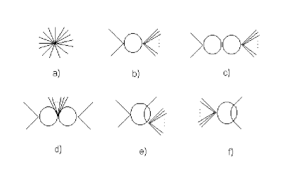
Figure 3: The graphs contributing to the vertex function $\Gamma^{(f)}_{*}$ up to 2-loop order. (a) represents the $f$-point vertex $[\phi]^{f}_{*}$, (b): one-loop contribution, (c)-(f): two-loop contributions.

The renormalized vertex functions $\Gamma_{R}^{(L,N)}$ and $\Gamma_{*R}^{(f)}$ are expressed in terms of the bare vertex functions as follows:

$$\Gamma_{R}^{(L,N)}(\{k\};\{p\};\hat{\mu}^{2};\{\lambda\})=$$

$$Z_{\phi^{2}}^{L}Z_{\phi}^{N/2}\Gamma_{0}^{(L,N)}(\{k\};\{p\};\hat{\mu}_{0}^{2};\{\lambda_{0}\}),$$

$$\Gamma_{*R}^{(f)}(\{k\};\hat{\mu}^{2};\{\lambda\})=$$

$$Z_{*f}\Gamma_{*0}^{(f)}(\{k\};\hat{\mu}_{0}^{2};\{\lambda_{0}\}),$$ (20)

where $Z_{\phi}$, $Z_{\phi^{2}}$, $Z_{*f}$ are the renormalizing factors, $\hat{\mu}$, $\{\lambda\}$ are the renormalized mass and couplings.

The change of couplings $u_{0},w_{0}$ under renormalization defines a flow in parametric space, governed by corresponding $\beta$-functions:

$$\beta_{u}(u,w)=\frac{\partial u}{\partial\ln\ell}\Big{|}_{0},\,\,\beta_{w}(u,w)=\frac{\partial w}{\partial\ln\ell}\Big{|}_{0},$$ (21)

where $l$ is the rescaling factor, and $\Big{|}_{0}$ stands for evaluation at fixed bare parameters. The fixed points (FPs) $u^{*},w^{*}$ of the RG transformation are given by the solution of the system of equations:

$$\beta_{u}(u^{*},w^{*})=0,\phantom{55}\beta_{w}(u^{*},w^{*})=0\,.$$ (22)

The stable FP, corresponding to the critical point of the system, is defined as the fixed point where the stability matrix

$$B_{ij}=\frac{\partial\beta_{\lambda_{i}}}{\partial\lambda_{j}}$$ (23)

possesses eigenvalues $\{\omega_{i}\}$ with positive real parts. The flow of the renormalizing factors $Z_{\phi}$, $Z_{\phi^{2}}$, $Z_{*f}$ in turn defines the corresponding RG functions:

$$\gamma_{\phi}(u,w) = \frac{\partial\ln Z_{\phi}}{\partial\ln\ell}\Big{|}_{0},$$ (24)

$${\bar{\gamma}}_{\phi^{2}}(u,w) = -\frac{\partial\ln{Z}_{\phi^{2}}}{\partial\ln\ell}\Big{|}_{0}-\gamma_{\phi},$$ (25)

$$\eta_{f}(u,w) = \frac{\partial\ln Z_{*f}}{\partial\ln\ell}\Big{|}_{0}.$$ (26)

The critical exponents are the values of these functions (24)–(26) at the stable accessible FP of Eq. (22):

$$\nu^{-1}=2-\gamma_{\phi}(u^{*},w^{*})-\bar{\gamma}_{\phi^{2}}(u^{*},w^{*}),$$ (27)

$$\eta=\gamma_{\phi}(u^{*},w^{*}),$$ (28)

$$\eta_{f}=\eta_{f}(u^{*},w^{*}),$$ (29)

$$\gamma_{f}=1+\nu\eta_{f}(u^{*},w^{*})+(\nu(2-\eta)-1)f.$$ (30)

Here, $\eta_{f}$ is the anomalous dimension of the composite operator $[\phi]^{f}_{*}$. The expressions for the exponents $\nu$, $\eta$ of a single polymer chain in long-range-correlated disorder we derived in Ref. Blavats’ka et al. (2001a, b); Blavats’ka et al. (2002). Only the RG functions $\eta_{f}$ that correspond to the anomalous dimensions of the composite operator $[\phi]^{f}_{*}$ in the presence of correlated disorder remain to be calculated in order to extract the spectrum of star polymer exponents $\gamma_{f}$ (given by Eq. (30)).

IV The results

The perturbative expansions for the functions (21), (24) - (26) may be analyzed by two complementary approaches: either by exploiting a double expansion in $\varepsilon=4-d,\delta=4-a$ Weinrib and Halperin (1983); Dorogovtsev (1984); Korutcheva and de la Rubia (1998); Blavats’ka et al. (2001a) or by evaluating the theory for fixed values of the parameters $d$ and $a$ Prudnikov and Fedorenko (1999); Prudnikov et al. (1999, 2000); Blavats’ka et al. (2001b); Blavats’ka et al. (2002). In the following we make use of both ways of analysis.

IV.1 One-loop approximation: $\varepsilon,\delta$ - expansion

For the qualitative analysis of the first order results, we apply a double expansion in $\varepsilon=4-d$ and $\delta=4-a$. First, we need to calculate the $f$-point vertex function $\Gamma^{(f)}_{*}$ with a single insertion of the composite operator $[\phi]_{*}^{f}$. In the one-loop approximation we get:

$$\Gamma^{(f)}_{*}(u_{0},w_{0},\{k\}=0,\hat{\mu}_{0})=1-u_{0}\,\frac{f(f-1)}{6}$$

$$\times\int\frac{{\rm d}{\vec{q}}}{(q^{2}+\hat{\mu}_{0}^{2})^{2}}+w_{0}\,\frac{f(f-1)}{6}\int\frac{{\rm d}{\vec{q}}\,q^{a-d}}{(q^{2}+\hat{\mu}_{0}^{2})^{2}}.$$ (31)

We define renormalized mass $\hat{\mu}^{2}$ and couplings $u,v$ by the renormalization conditions:

$$\hat{\mu}^{2} = \Gamma_{R}^{(2)}(k,\hat{\mu}^{2},u,w)|_{k=0},$$

$$u = \Gamma_{R,u}^{(4)}(\{k\},\hat{\mu}^{2},u,w)|_{\{k\}=0},$$

$$w = \Gamma_{R,w}^{(4)}(\{k\},\hat{\mu}^{2},u,w)|_{\{k\}=0}.$$

The renormalization condition for the vertex function with $[\phi]_{*}^{f}$-insertion is given by

$$Z_{*f}(u,w) = [\Gamma^{(f)}_{*}(u,w)]^{-1}$$ (32)

$$=1+u\frac{f(f-1)}{6}I_{1}-w\frac{f(f-1)}{6}I_{2}\,.$$

Here, $I_{1}$ and $I_{2}$ are loop integrals given in the appendix. The expressions for the RG $\beta$- and $\gamma$-functions (21), (24), (25) within the same approximation read Blavats’ka et al. (2001a):

$$\beta_{u} = -\varepsilon\left[u-\frac{4}{3}\,u^{2}I_{1}\right]-\delta 2uw\left[I_{2}-\frac{1}{3}D_{1}\right]$$ (33)

$$+ (2\delta-\varepsilon)\frac{2}{3}\,w^{2}I_{3},$$

$$\beta_{w} = -\delta\left[w+\frac{2}{3}\,w^{2}I_{2}+w^{2}D_{1}\right]+\varepsilon\frac{2}{3}\left[wuI_{1}\right],$$ (35)

$$\gamma_{\phi^{2}}=\varepsilon\frac{u}{3}\,I_{1}-\delta\,\frac{w}{3}\,I_{2},\phantom{55}\gamma_{\phi}=\delta\,\frac{w}{3}D_{1}.$$

Again, the loop integrals $I_{1}-I_{3},D_{1}$ are given in the Appendix. Note that contrary to the usual $\phi^{4}$ theory the $\gamma_{\phi}$ function in Eq. (35) is nonzero already in the one-loop order. This is due to the $k$-dependence of the integral $D_{1}$. Combining Eqs. (26) and (21) one defines $\eta_{f}$ via familiar expressions (32) and (35):

$$\eta_{f}=\beta_{u}(u,w)\frac{\partial\ln Z_{*f}}{\partial u}+\beta_{w}(u,w)\frac{\partial\ln Z_{*f}}{\partial w}.$$ (36)

To proceed with the analysis, we insert the expansions of the one-loop integrals:

$$I_{1} = \frac{1}{\varepsilon}\left(1-\frac{\varepsilon}{2}\right),$$ (37)

$$I_{2} = \frac{1}{\delta}\left(1-\frac{\delta}{2}\right),$$ (38)

$$I_{3} = \frac{1}{2\delta-\varepsilon}\left(1-\frac{2\delta-\varepsilon}{2}\right),$$ (39)

$$D_{1} = \frac{1}{\delta}\left(\frac{\delta-\varepsilon}{2}\right).$$ (40)

Substituting (37) - (40) into the expressions for $\beta$-functions (33), (35) and solving the FP equation (22), one finds three fixed points: the Gaussian ($u^{*}=0,w^{*}=0$), the pure ($u^{*}=\frac{3}{4}\varepsilon,w^{*}=0)$, and the non-trivial, long-range-correlated, LR fixed point: ($u^{*}=\frac{3}{4}\frac{2\delta^{2}}{\varepsilon-\delta},w^{*}=\frac{3}{2}\frac{\delta(\varepsilon-2\delta)}{\delta-\varepsilon}$). The analysis of the conditions of their stability and accessibility we performed in Ref. Blavats’ka et al. (2001a). The results are displayed schematically in Fig. 4: at $\varepsilon,\delta>0$, the crossover from the pure FP to the LR takes place at $\delta=\varepsilon/2,$ i.e. $a=2+d/2$. Note, however, that the LR FP is stable in the region $a>d$, where the influence of the disorder is expected to be irrelevant, see the explanation after Eq. (17). These first order results give a qualitative description of the crossover to the new universality class in the presence of long-range-correlated disorder.

The expression for the critical exponent $\nu$ reads Blavats’ka et al. (2001a):

$$\nu = \left\{\begin{array}[]{ll}\nu^{(0)}=1/2+\varepsilon/16,&\delta<\varepsilon/2,\\ \nu^{(\delta)}=1/2+\delta/8,&\varepsilon/2<\delta<\varepsilon.\end{array}\right.$$ (43)

From (36) we find:

$$\eta_{f} = \left\{\begin{array}[]{ll}\eta_{f}^{(0)}=-\frac{1}{8}\varepsilon f(f-1),&\delta<\varepsilon/2,\\ \eta_{f}^{(\delta)}=-\frac{1}{4}\delta f(f-1),&\varepsilon/2<\delta<\varepsilon,\end{array}\right.$$ (46)

Figure 4: Fixed point picture for $d<4$, $a>d$. Stable physically accessible fixed points are shown by squares the unstable ones by discs. (a): $\delta<\varepsilon/2$, the pure fixed point ($u^{*}\neq 0,w^{*}=0$) is stable. At $\delta=\varepsilon/2$, it interchanges its stability with the LR fixed point ($u^{*}\neq 0,w^{*}\neq 0$). (b): for $\varepsilon/2<\delta<\varepsilon$ the LR fixed point becomes physically accessible and stable. The Gaussian fixed point ($u^{*}=0,w^{*}=0$) is stable for $d>4,a>4$.

Substituting (46), (43) into (30), finally we get:

$$\gamma_{f}=\left\{\begin{array}[]{ll}\gamma_{f}^{(0)}=1-\frac{1}{16}\varepsilon f(f-3)&\delta<\varepsilon/2,\\ \gamma_{f}^{(\delta)}=1-\frac{1}{8}\delta f(f-3)&\varepsilon/2<\delta<\varepsilon,\end{array}\right.$$ (49)

The first line in (49) recovers the exponent for the $f$-arm polymer star in the pure solution Miyake and Freed (1983), whereas the second line brings about a new scaling law.

To obtain a naive estimate of the numerical values of these exponents, one can directly substitute into (49) the value $\varepsilon=1$ (corresponding to $d=3$) and different fixed values for correlation parameter $a$ We note a decrease of the star exponent $\gamma_{f}$ at fixed $f>3$, when the correlation of the disorder becomes stronger (i.e. parameter $a$ decreases). However, the behavior for chain polymers i.e. for $f=1,2$ differs: in this case the exponents $\gamma_{1}=\gamma_{2}$ increase for decreasing $a$.

Figure 5: Comparison of the exponents $\gamma_{f}$ for star polymers in a pure solution (continuous line) and in a solution inside a correlated porous medium (broken line), following Eq.(49) for $\varepsilon=1$, $\delta=0.9$.

This crossover is also clearly seen in Fig. 5 where we compare the behavior of $\gamma_{f}$ for the case with and without correlated disorder.As this figure shows, the correlation of the disorder effectively enhances the deviation from the mean field value $\gamma_{f}^{\rm MF}=1$ which is positive for $f=1,2$ and negative for $f>3$ in this approximation.

IV.2 Two-loop approximation: fixed $d,a$ approach

To obtain a quantitative description of the scaling behavior of star polymers in long-range-correlated disorder, we proceed to higher order approximations. We make use of the fixed $d=3$ RG approach Parisi (1980), considering the massive RG functions at fixed space dimension $d$. Also the additional parameter $a$ in the expansions for the RG functions in renormalized couplings $u$, $w$ (21), (24)-(26) is fixed in this approach and we work hereafter with these expansions. As is well known Brezin et al. (1976); Zinn-Justin (1996); Kleinert and Schulte-Frohlinde (2001), such expansions are in general characterized by a factorial growth of the coefficients which implies a zero radius of convergence Hardy (1948). No reliable data can be extracted from a naive analysis. For the present model, this particular feature shows up already in the first order of perturbation theory in $u$ and $w$. Indeed, for the plain one-loop $\beta$-functions (35) a non-trivial FP LR does not appear if one solves the non-linear fixed point equation (22) directly at $d=3$ and $2<a<3$. To take into account higher order contributions, the standard tools of asymptotic series resummation have to be applied Hardy (1948).

The two-variable Padé-Borel resummation technique Jug (1983) that we use consists of several steps. Consider the two-variable series for a RG function $h(u,w)$. First, we construct the Borel image of the initial function:

$$h(u,w)=\sum_{i,j}a_{i,j}u^{i}w^{j}\to\sum_{i,j}\frac{a_{i,j}(ut)^{i}(wt)^{j}}{\Gamma(i+j+1)},$$

where $\Gamma(i+j+1)$ is Euler’s gamma function. Then, the Borel image is extrapolated by a rational Padé approximant $[K/L](u,w)$. This ratio of two polynomials of order $K$ and $L$ is constructed as to match its truncated Taylor expansion to that of the Borel image of the function $h(u,w)$. The resummed function is then recovered by an inverse Borel transform of this approximant:

$$h^{\rm res}(u,w)=\int_{0}^{\infty}{\rm d}t\exp(-t)[K/L](ut,wt).$$ (50)

In our previous work Blavats’ka et al. (2001b); Blavats’ka et al. (2002) we have analyzed the resummed expressions for the two-loop RG functions of the model of a single polymer chain in the long-range-correlated disorder in three dimensions, and found that a fixed point LR appears and is stable at $2.2<a<3$. This FP disappears at $a<2.2$ and the pure SAW FP remains unstable. This behavior may be interpreted to indicate, that the presence of stronger correlated disorder (at $a<2.2$) might lead to a collapse of the polymer chain. To obtain a quantitative picture of the scaling behavior of star polymers, we only need to extend these results by a calculation of the renormalization factor $Z_{*f}$ (36). Taking into account the two-loop contributions shown in Fig. 3 we get:

$$Z_{*f} = 1+u\,\frac{f(f-1)}{6}I_{1}-w\,\frac{f(f-1)}{6}I_{2}$$ (51)

$$+u^{2}\,f(f-1)\left[\left(-\frac{1}{72}(f-2)(f-3)\right.\right.\left.+\frac{1}{36}f(f-1)+\frac{1}{6}\right)I_{1}^{2}$$

$$-\left(\frac{f-2}{9}+\frac{1}{6}\right)I_{6}\Big{]}-uw\,f(f-1)\left[\left(-\frac{1}{36}(f-2)(f-3)+\frac{1}{18}f(f-1)\right.\right.\left.+\frac{7}{8}\right)I_{1}I_{2}$$

$$+\left(-\frac{1}{9}(f-2)-\frac{1}{3}\right)I_{7}-\left.\frac{1}{9}(f-2)I_{9}-\frac{I_{4}}{18}-\frac{2}{3f(f-1)}D_{1}\right]$$

$$+w^{2}\,f(f-1)\left[\left(-\frac{(f-2)(f-3)}{72}-\frac{f(f-1)}{36}\right.\right.$$

$$+\frac{1}{9}\left.\right)I_{2}^{2}-\left(\frac{f-2}{18}+\frac{1}{6}\right)I_{8}-\frac{f-2}{18}I_{10}+\frac{1}{9}I_{3}I_{1}-\left.\frac{1}{18}I_{5}-\frac{2}{3f(f-1)}I_{2}D_{1}\right].$$

The expressions for the loop integrals $I_{1},\ldots,I_{10},D_{1}$ and their numerical values at $d=3$ and different $a$ are presented in the Appendix.

In this way, the function $\eta_{f}$ can be found, using (36) and familiar expressions for the two-loop $\beta$-functions as given in Blavats’ka et al. (2001b); Blavats’ka et al. (2002). The resulting two-loop expansion for $\eta_{f}$ reads not :

$$\eta_{f} = -u\frac{f(f-1)}{8}-w\frac{(4-a)f(f-1)}{8}I_{2}/I_{1}$$

$$+u^{2}\left(\left(-\frac{f^{3}}{16}+\frac{3f^{2}}{32}-\frac{f}{32}\right)I_{1}^{2}+\left(\frac{f^{3}}{8}-\frac{3}{16}f^{2}+\frac{f}{16}\right)I_{6}\right)\Big{/}I_{1}^{2}$$

$$+uw\Big{(}\left(-\frac{f^{3}}{16}(1+(4-a))+\frac{f}{16}(1-(4-a))+(4-a)\frac{f^{2}}{8}\right)I_{1}I_{2}$$

$$+\left((1+(4-a))\left(\frac{f^{3}}{16}-\frac{3f^{2}}{32}+\frac{f}{32}\right)\right)(I_{7}+I_{9})$$

$$+\left((1+(4-a))\left(\frac{f^{2}}{32}-\frac{f}{32}\right)\right)I_{4}$$

$$+\left(\frac{3}{8}(1+(4-a))\right.-\left.\frac{f^{2}(4-a)}{16}+\frac{(4-a)f}{16}\right)\frac{I_{1}D_{1}}{f(f-1)})\Big{/}I_{1}^{2}$$

$$+w^{2}\Big{(}\left(-\frac{f^{2}}{16}-\frac{f}{16}\right)I_{1}I_{3}+\frac{(4-a)f(f-1)}{16}I_{5}+$$

$$+\frac{(4-a)(f-1)(f+1)}{16}I_{8}+\frac{(4-a)f(f-1)(f-2)}{16}I_{10}$$

$$+\left((4-a)-\frac{f^{2}}{16}+\frac{f}{6}+\frac{3}{4}\right)I_{2}D_{1}\Big{)}\Big{/}I_{1}^{2}\,.$$

Inserting the series for $\nu$ and $\eta$ for the polymer chain in the long-range-correlated disorder from Refs. Blavats’ka et al. (2001b); Blavats’ka et al. (2002) together with $\eta_{f}$ of Eq. (IV.2) into (30), we finally obtain the corresponding series for $\gamma_{f}$. Substituting the numerical values of the LR correlated FP, found for different $a$ from Refs. Blavats’ka et al. (2001b); Blavats’ka et al. (2002) and applying a Padé-Borel resummation as explained above we get the numerical values for exponents $\gamma_{f}$ in three dimensions for different values of the correlation parameter $a$ and number of arms $f$. Our final estimates that result from this procedure are presented in Table 1. For $f=3$, the first order contribution to $\gamma_{f}$ is zero, whereas it is non-zero for $\eta_{3}$. Therefore, to obtain a resummed value for $\gamma_{3}$ we have resummed the series for $\eta_{3}$ using the values for $\eta$ and $\nu$ of chain polymers in long-range-correlated disorder.

$a\setminus f$	1;2	3	4	5	6	7	8	9
3, von Ferber and Holovatch (1995, 1996)	1.18	1.06	0.86	0.61	0.32	-0.02	-0.4	-0.8
3, Hsu et al. (2004)	1.1573(2)	1.0426(7)	0.8355(10)	0.5440(12)	0.1801(20)	-0.2520(25)	-0.748(3)	-1.306(5)
3	1.17	0.99	0.83	0.57	0.26	-0.08	-0.56	-0.87
2.9	1.25	0.87	0.78	0.46	0.09	-0.32	-0.76	-1.23
2.8	1.26	0.81	0.76	0.43	0.06	-0.36	-0.80	-1.26
2.7	1.28	0.74	0.72	0.40	0.01	-0.40	-0.85	-1.31
2.6	1.30	0.73	0.70	0.37	-0.03	-0.46	-0.91	-1.37
2.5	1.34	0.71	0.70	0.35	-0.10	-0.51	-1.00	-1.44
2.4	1.35	0.70	0.70	0.31	-0.10	-0.55	-1.02	-1.50
2.3	1.38	0.70	0.69	0.29	-0.13	-0.59	-1.06	-1.55

Table 1: Critical exponents $\gamma_{f}$ for the $f$-armed star in three dimensions at different values of the correlation parameter $a$. The first and the second rows ($a=d=3$) present results for a polymer star in a good solvent without porous medium obtained within the field-theoretical RG in three-loop approximation, Ref. von Ferber and Holovatch (1995, 1996), and by the Monte Carlo simulations, Ref. Hsu et al. (2004), correspondingly.

Let us recall, that for $a=d=3$ the problem is equivalent to the situation without structural disorder. Therefore, in the first two rows of Table 1 we give RG estimates for the exponents $\gamma_{f}$ obtained in a three-loop approximation in Ref. von Ferber and Holovatch (1995, 1996) as well as recent data of MC simulations Hsu et al. (2004). Comparing these data with our two-loop results (the third row of the Table) allows to estimate the consistency of the calculational scheme that we apply. The good mutual agreement found for the low values of $f$ supports our approach. The fact that the discrepancy increases with $f$ is expected, taking into account the strong combinatorial $f$-dependence of the coefficients of expansions (51), (IV.2). This growth is difficult to control in a consistent way during the resummation.

As we noted above, the choice $f=1,f=2$ recovers the case of a single polymer chain. Therefore, the first and the second columns of Table 1 give an estimate for the dependence of the exponent $\gamma$, Eq. (1): $\gamma^{(a)}=\gamma_{1}^{(a)}=\gamma_{2}^{(a)}$. The remarkable feature of the estimates for $\gamma_{f}^{(a)}$ listed in the Table 1 is that they predict a qualitatively different behavior of $\gamma_{f}^{(a)}$ for $f=1,f=2$ and $f\geq 3$. Indeed, as one sees from Table 1, a decrease in $a$ leads to an increase of $\gamma_{1}^{(a)},\gamma_{2}^{(a)}$ while $\gamma_{f}^{(a)}$ for $f\geq 3$ decrease in this case. This tendency is also found for the one-loop $\varepsilon,\delta$-expansion (Eq. (49)).

Recall, that the scaling exponent of a star polymer in a pure solvent is given by $\gamma_{f}^{(a=3)}$ and let us return back to Eqs. (7) and (8) for the free energy of a star in the pure solvent and in a porous medium. Then our results indicate two different regimes of the entropy-induced change of the polymer concentration for a solvent in a porous medium with respect to the pure one. Namely, the free energy of the chain polymers ($f=1,f=2$) is reduced by the presence of correlation in a porous medium. On the other hand, the free energy of a star polymer ($f\geq 3$) is increased by correlations of the environment.

$a$	$\Theta_{41}$	$\Theta_{43}$	$\Theta_{44}$	$\Theta_{45}$	$\Theta_{46}$	$\Theta_{47}$	$\Theta_{48}$	$\Theta_{49}$
2.9	1.306	1.627	1.865	2.042	2.220	2.348	2.402	2.531
2.8	1.286	1.565	1.777	1.932	2.071	2.163	2.246	2.345
2.7	1.262	1.502	1.691	1.817	1.941	2.024	2.082	2.166
2.6	1.239	1.459	1.608	1.739	1.843	1.910	1.987	2.040
2.5	1.229	1.410	1.554	1.668	1.762	1.834	1.876	1.929
2.4	1.217	1.392	1.521	1.617	1.705	1.758	1.799	1.883
2.3	1.193	1.360	1.474	1.574	1.651	1.707	1.725	1.772

Table 2: Contact exponents $\Theta_{ff}$, governing the scaling behavior of interaction force between two $f$- and $f^{\prime}$-armed polymer star in three dimensions at different values of the correlation parameter $a$.

To investigate the influence of a porous medium on the effective interactions between star polymers we calculate the contact exponents $\Theta_{ff^{\prime}}$ (Eq. 4). Our results, obtained by a Padé-Borel resummation of the series derived from Eq. (5). are presented in Figs. 6, 7 and for a selected set of exponents also in Table 2. In Fig. 5 we show the contact exponent $\Theta_{ff}$ for two stars of the same number of arms $f$ as a function of $a$ and $f$. The exponent increases with increasing of $f$ and $a$ for $f\geq 3$. Fig. 6 presents $\Theta_{ff^{\prime}}$ for a fixed $a$ (we have chosen $a=2.7$ for an illustration). For fixed $f,f^{\prime}$, this exponent decreases with the decrease of the correlation parameter $a$. Thus, we can conclude, that polymer stars interact more weakly in media with strong correlated disorder.

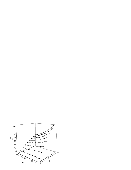
Figure 6: The contact exponent $\Theta_{ff}$ as function of $f$ and correlation parameter $a$ at $d=3$. Each line shows the dependence of $\Theta_{ff}$ on $a$ at fixed $f$.

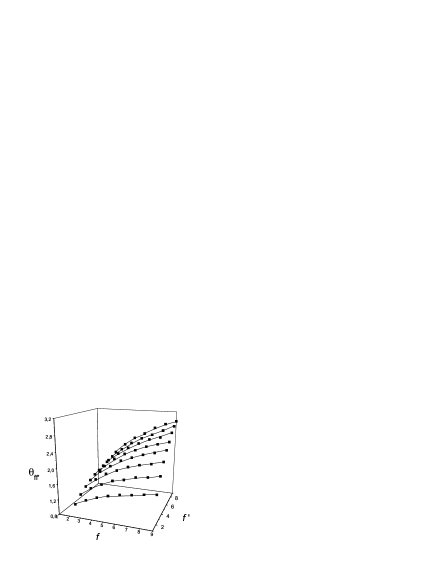
Figure 7: The contact exponent $\Theta_{ff^{\prime}}$ as function of $f$ and $f^{\prime}$ for fixed correlation parameter $a=2.7$ at $d=3$.

V Conclusions

The present study provides numerical estimates for the spectrum of critical exponents that govern the scaling behavior of the $f$-arm star polymers in a good solvent in the presence of a correlated disordered medium, characterized by a correlation function $g(r)\sim r^{-a}$ at large distances $r$. This extends previous results Blavats’ka et al. (2001a, b); Blavats’ka et al. (2002) that have shown that the scaling behavior of polymer chains in this type of disorder belongs to a new universality class.

Working within the field-theoretical RG approach, we applied both a double expansion in $\varepsilon=4-d$ and $\delta=4-a$ as well as a technique that evaluates the perturbation series for fixed $d,a$. The first one-loop analysis allowed us to identify a quantitatively new behavior in comparison with the pure case. The second approach, refined by a resummation of the resulting divergent series, resulted in numerical quantitative estimates for the scaling exponents. We found the numerical values of the exponents $\gamma_{f}$ in three-dimensional case for different fixed values of the correlation parameter $2.3\leq a\leq 2.9$, and for fixed numbers of arms $f=1,\ldots,9$. Depending on the value of $f$, we find two different regimes of the entropy-induced effects on the polymer in a correlated porous medium. While an increase of the correlation of the disorder causes the free energy of chain polymers ($f=1,f=2$) to decrease, the same change in correlation rather leads to an increase in the free energy for star polymers ($f\geq 3$). Therefore, for a mixture of chain and star polymers of equal molecular mass (same total number of effective monomers) in a solution for which a part of the volume is influenced by a porous medium the disorder-influenced part of the solvent is predicted to be enriched by chain polymers. Correspondingly, the relative concentration of star polymers to and chain polymers will be lower in the porous medium.

From our numerical estimates for contact exponents $\Theta_{ff^{\prime}}$, we deduce the influence of the correlated disorder for the effective interaction between star polymers. Again we find different behavior for chain and star polymers. While for chain polymers the effective contact interaction increases for decreasing $a$, i.e. for enhanced correlation, the mutual interaction between star polymers is weakened in correlated media.

VI Appendix

Here, we present the expressions for the loop integrals, as they appear in the RG functions. We make the couplings dimensionless by redefining $u=u\hat{\mu}^{d-4}$ and $w=w\hat{\mu}^{a-4}$. Therefore, the loop integrals do not explicitly contain the mass.

$$I_{1}=\int\frac{{\rm d}{\vec{q}}}{(q^{2}+1)^{2}};$$

$$I_{2}=\int\frac{{\rm d}{\vec{q}}\,q^{a-d}}{(q^{2}+1)^{2}};$$

$$I_{3}=\int\frac{{\rm d}{\vec{q}}\,q^{2(a-d)}}{(q^{2}+1)^{2}};$$

$$I_{4}=\int\int\frac{{\rm d}{\vec{q}_{1}}{\rm d}{\vec{q}_{2}}\,q_{1}^{(a-d)}}{(q_{2}^{2}+1)^{2}((q_{1}-q_{2})^{2}+1)^{2}};$$

$$I_{5}=\int\int\frac{{\rm d}{\vec{q}_{1}}{\rm d}{\vec{q}_{2}}\,q_{1}^{(a-d)}\,q_{2}^{a-d}}{(q_{2}^{2}+1)^{2}((q_{1}-q_{2})^{2}+1)^{2}};$$

$$I_{6}=\int\int\frac{{\rm d}{\vec{q}_{1}}{\rm d}{\vec{q}_{2}}}{(q_{1}^{2}+1)(q_{2}^{2}+1)^{2}((q_{1}-q_{2})^{2}+1)^{2}};$$

$$I_{7}=\int\int\frac{{\rm d}{\vec{q}_{1}}{\rm d}{\vec{q}_{2}}\,q_{1}^{a-d}}{(q_{1}^{2}+1)(q_{2}^{2}+1)^{2}((q_{1}-q_{2})^{2}+1)};$$

$$I_{8}=\int\int\frac{{\rm d}{\vec{q}_{1}}{\rm d}{\vec{q}_{2}}\,q_{1}^{a-d}q_{2}^{(a-d)}}{(q_{1}^{2}+1)(q_{2}^{2}+1)^{2}((q_{1}-q_{2})^{2}+1)};$$

$$I_{9}=\int\int\frac{{\rm d}{\vec{q}_{1}}{\rm d}{\vec{q}_{2}}\,q_{1}^{a-d}}{(q_{1}^{2}+1)^{2}(q_{2}^{2}+1)((q_{1}-q_{2})^{2}+1)};$$

$$I_{10}=\int\int\frac{{\rm d}{\vec{q}_{1}}{\rm d}{\vec{q}_{2}}\,q_{1}^{2(a-d)}}{(q_{1}^{2}+1)^{2}(q_{2}^{2}+1)((q_{1}-q_{2})^{2}+1)};$$

$$D_{1}=\frac{\partial}{\partial k^{2}}\left[\int\frac{{\rm d}\vec{q}\,q^{a-d}}{[q+k]^{2}+1)}\right]_{k^{2}=0}.$$ (53)

The correspondence of the integrals to the diagrams in Fig. 3 is: (b): integrals $I_{1},I_{2},I_{3}$, $(c)$: $I_{4},I_{5}$; $(d)$: $I_{1}I_{2}$, $I_{2}^{2}$; $e$: $I_{6},I_{7},I_{8},I_{9},I_{10}$; $(f)$: $I_{6},I_{7},I_{8},I_{9}$. In our calculations, we use the following formulas for folding many denominators into one (see e.g. Amit (2.ed.1984)):

$$\frac{1}{a_{1}^{\alpha_{1}}\ldots a_{n}^{\alpha_{n}}}=\frac{\Gamma(\alpha_{1}{+}\ldots{+}\alpha_{n})}{\Gamma(\alpha_{1})\ldots\Gamma(\alpha_{n})}$$ (54)

$$\int\limits_{0}^{1}{\rm d}x_{1}\!\!\ldots\!\!\int\limits_{0}^{1}{\rm d}x_{n-1}\frac{x_{1}^{\alpha_{n}-1}\ldots x_{n-1}^{\alpha_{n-1}-1}(1{-}x_{1}{-}\ldots{-}x_{n-1})^{\alpha_{n}-1}}{(x_{1}a_{1}{+}\ldots{+}x_{n-1}a_{n-1}{+}(1{-}x_{1}{-}\ldots{-}x_{n-1})a_{n})^{\alpha_{1}+\ldots+\alpha_{n}}}$$

To compute the $d$-dimensional integrals we apply

$$\int\limits_{0}^{\infty}\frac{{\rm d}q\,q^{d-1}}{(q^{2}+2\vec{k}\vec{q}+m^{2})^{\alpha}}=$$

$$\frac{1}{2}\frac{\Gamma(d/2)\Gamma(\alpha-d/2)}{\Gamma(\alpha)}(m^{2}-k^{2})^{d/2-\alpha}$$ (55)

As an example we present the calculation of the integral $I_{7}$. First, we make use of formula (54) to rewrite:

$$\frac{1}{(q_{1}^{2}+1)((q_{1}-q_{2})^{2}+1)}=$$

$$\frac{\Gamma(2)}{\Gamma(1)\Gamma(1)}\int_{0}^{1}\frac{{\rm d}x}{(q_{1}^{2}+2x\vec{q_{1}}\vec{q_{2}}+xq_{2}^{2}+1)^{2}}.$$ (56)

Now one can perform integration over $q_{1}$, passing to the $d$-dimensional polar coordinates and making use of the formula (55):

$$\int\frac{{\rm d}\vec{q_{1}}\,q_{1}^{a-d}}{(q_{1}^{2}+2x\vec{q_{1}}\vec{q_{2}}+xq_{2}^{2}+1)^{2}}=$$

$$C\int\limits_{0}^{\infty}\frac{{\rm d}q_{1}\,q_{1}^{a-1}}{(q_{1}^{2}+2x\vec{q_{1}}\vec{q_{2}}+xq_{2}^{2}+1)^{2}}=$$

$$\frac{1}{2}\frac{\Gamma(a/2)\Gamma(2-a/2)}{\Gamma(2)}(1+q_{2}^{2}x(1-x))^{a/2-2},$$ (57)

where the constant $C=(2\pi)^{d/2}/\Gamma(d/2)$ results from integration over the angular variables. It does not appear explicitly in the following expressions. Finally, we are left with:

$$I_{7} = \frac{1}{2}{\Gamma(a/2)}{\Gamma(2-a/2)}$$ (58)

$$\int_{0}^{\infty}\frac{{\rm d}q_{2}\,q_{2}^{d-1}}{(q_{2}^{2}+1)^{2}}\int\limits_{0}^{1}{\rm d}x(1+q_{2}^{2}x(1-x))^{a/2-2},$$

this integral was calculated numerically, fixing the values of the parameters $d,a$ using the MAPLE package. Note that some of the integrals can also be evaluated analytically.

$a$	$I_{1}$	$I_{2}$	$I_{3}$	$I_{4}$	$I_{5}$	$I_{6}$	$I_{7}$	$I_{8}$	$I_{9}$	$I_{10}$	$D_{1}$
2.9	0.7855	0.7155	0.6605	0.5621	0.5119	0.4114	0.3643	0.3477	0.3916	0.3756	0.0052
2.8	0.7855	0.6605	0.5825	0.5187	0.4363	0.4114	0.3274	0.3016	0.3756	0.3525	0.0012
2.7	0.7855	0.6170	0.5345	0.4848	0.3807	0.4114	0.2981	0.2677	0.3626	0.3395	0.0015
2.6	0.7855	0.5825	0.5085	0.4575	0.3393	0.4114	0.2746	0.2425	0.3525	0.3357	0.0021
2.5	0.7855	0.5550	0.5000	0.4361	0.3080	0.4114	0.2555	0.2238	0.3448	0.3408	0.0027
2.4	0.7855	0.5345	0.5085	0.4198	0.2857	0.4114	0.2406	0.2106	0.3395	0.3557	0.0034
2.3	0.7855	0.5185	0.5345	0.4075	0.2688	0.4114	0.2283	0.2014	0.3365	0.3823	0.0041

Table 3: The numerical values for loop integrals $I_{i}$ for $d=3$ and different values of the correlation parameter $a$.

Below, we list the results for all the integrals.

$$I_{1} = \frac{1}{2}\Gamma(d/2)\Gamma(2-d/2),$$

$$I_{2} = \frac{1}{2}\Gamma(a/2)\Gamma(2-a/2),$$

$$I_{3} = \frac{1}{2}\Gamma((2a-d)/2)\Gamma(2-(2a-d)/2),$$

$$I_{4} = \frac{1}{4}\Gamma(a/2)\Gamma(d/2)\Gamma(2-a/2)\Gamma(2-d/2),$$

$$I_{5} = \frac{1}{4}\Gamma(a/2)\Gamma(a/2)\Gamma(2-a/2)\Gamma(2-a/2),$$

$$I_{6} = \frac{1}{2}{\Gamma(d/2)}{\Gamma(2-d/2)}\times$$

$$\int_{0}^{\infty}\frac{{\rm d}q_{2}\,q_{2}^{d-1}}{(q_{2}^{2}+1)^{2}}\int\limits_{0}^{1}{\rm d}x(1+q_{2}^{2}x(1-x))^{d/2-2},$$

$$I_{8} = \frac{1}{2}{\Gamma(a/2)}{\Gamma(2-a/2)}\times$$

$$\int_{0}^{\infty}\frac{{\rm d}q_{2}\,q_{2}^{a-1}}{(q_{2}^{2}+1)^{2}}\int\limits_{0}^{1}{\rm d}x(1+q_{2}^{2}x(1-x))^{a/2-2},$$

$$I_{9} = \frac{1}{2}{\Gamma(d/2)}{\Gamma(2-d/2)}\times$$

$$\int_{0}^{\infty}\frac{{\rm d}q_{2}\,q_{2}^{a-1}}{(q_{2}^{2}+1)^{2}}\int\limits_{0}^{1}{\rm d}x(1+q_{2}^{2}x(1-x))^{d/2-2},$$

$$I_{10} = \frac{1}{2}{\Gamma(d/2)}{\Gamma(2-d/2)}$$

$$\int_{0}^{\infty}\frac{{\rm d}q_{2}\,q_{2}^{2a-d-1}}{(q_{2}^{2}+1)^{2}}\int\limits_{0}^{1}{\rm d}x(1+q_{2}^{2}x(1-x))^{d/2-2},$$

$$D_{1} = \frac{(a-2)(a-3)(a-4)}{192\sin(\pi(1/2a-1))}.$$

Note, that the analytical value for $D_{1}$ is taken from Prudnikov and Fedorenko (1999); Prudnikov et al. (1999, 2000).

References

- Chakrabarti (2005) B. K. Chakrabarti, Statistics of Linear Polymers in Disordered Media (Elsevier, Amsterdam, 2005).
- Barat and Chakrabarti (1995) K. Barat and B. K. Chakrabarti, Phys. Rep. 258, 377 (1995).
- Harris (1983) A. B. Harris, Z. Phys. B 49, 347 (1983).
- Kim (1983) Y. Kim, J. Phys. C 16, 1345 (1983).
- Kremer (1981) K. Kremer, Z. Phys. B 45, 149 (1981).
- Meir and Harris (1989) Y. Meir and A. B. Harris, Phys. Rev. Lett. 63, 2819 (1989).
- Nakanishi and Lee (1991) H. Nakanishi and S. B. Lee, J. Phys. A 24, 1355 (1991).
- Grassberger (1993) P. Grassberger, J. Phys. A 26, 1023 (1993).
- Ordemann et al. (2000) A. Ordemann, M. Porto, H. E. Roman, S. Havlin, and A. Bunde, Phys. Rev. E 61, 6858 (2000).
- Blavats’ka et al. (2001a) V. Blavats’ka, C. von Ferber, and Y. Holovatch, J. Mol. Liq. 92, 77 (2001a).
- von Ferber et al. (2004) C. von Ferber, V. Blavats’ka, R. Folk, and Y. Holovatch, Phys. Rev. E 70, 035104(R) (2004).
- Blavats’ka et al. (2001b) V. Blavats’ka, C. von Ferber, and Yu. Holovatch, Phys. Rev. E 64, 041102 (2001b).
- Blavats’ka et al. (2002) V. Blavats’ka, C. von Ferber, and Yu. Holovatch, J. Phys.: Condens. Matter 14, 9465 (2002).
- Chan et al. (1988) M. H. W. Chan, K. I. Blum, S. Q. Murphy, G. K. S. Wong, and J. D. Reppy, Phys. Rev. Lett. 61, 1950 (1988).
- Li and Sieradzki (1992) R. Li and K. Sieradzki, Proc. Phys. Soc. Lond. 68, 1168 (1992).
- Gelb and Gubbins (1998) L. D. Gelb and K. E. Gubbins, Proc. Phys. Soc. Lond. 14, 2097 (1998).
- Yoon and Chan (1997) J. Yoon and M. H. W. Chan, Proc. Phys. Soc. Lond. 78, 4801 (1997).
- Vacher et al. (1988) R. Vacher, T. Woignier, J. Pelous, and E. Courtens, Phys. Rev. B 37, 6500 (1988).
- Yoon et al. (1998) J. Yoon, D. Sergatskov, J. A. Ma, N. Mulders, and M. H. W. Chan, Phys. Rev. Lett. 80, 1461 (1998).
- Pekala and Hrubesh (1995) R. W. Pekala and L. W. Hrubesh, Proceedings of the IV Int. Symp. on Aerogeles, vol. 186 of L. Non.-Cryst. Solids (1995).
- Grest et al. (1996) G. S. Grest, L. J. Fetters, J. S. Huang, and D. Richter, Advan. Chem. Physics 94, 67 (1996).
- Likos (2001) C. N. Likos, Phys. Rep. 348, 267 (2001).
- von Ferber and Holovatch (2002) C. von Ferber and Yu. Holovatch, eds., Special Issue “Star Polymers”, vol. 5 of Condens. Matter Phys. (2002).
- Duplantier (1989) B. Duplantier, J. Stat. Phys. 54, 581 (1989).
- Schäfer et al. (1992) L. Schäfer, C. von Ferber, U. Lehr, and B. Duplantier, Nucl. Phys. B 374, 473 (1992).
- Roovers and Bywater (1972) J. E. L. Roovers and S. Bywater, Macromolecules 5, 384 (1972).
- Roovers et al. (1983) J. Roovers, N. Hadjichristidis, and L. J. Fetters, Macromolecules 16, 214 (1983).
- Khasat et al. (1988) N. Khasat, R. W. Pennisi, N. Hadjichristidis, and L. J. Fetters, Macromolecules 21, 1100 (1988).
- Bauer et al. (1989) B. J. Bauer, L. J. Fetters, W. W. Graessley, N. Hadjichristidis, and G. F. Quack, Macromolecules 22, 2337 (1989).
- Merkle et al. (1993) G. Merkle, W. Burchard, P. Lutz, K. F. Freed, and J. Gao, Macromolecules 26, 2736 (1993).
- Grest et al. (1987) G. S. Grest, K. Kremer, and T. A. Witten, Macromolecules 20, 1376 (1987).
- Batoulis and Kremer (1989) J. Batoulis and K. Kremer, Macromolecules 22, 4277 (1989).
- Ohno (1994) K. Ohno, Macromol. Symp. 81, 121 (1994).
- Shida et al. (1996) K. Shida, K. Ohno, M. Kimura, and Y. Kawazoe, J. Chem. Phys. 105, 8929 (1996).
- Barrett and Tremain (1987) A. J. Barrett and D. L. Tremain, Macromolecules 20, 1687 (1987).
- Hsu et al. (2004) H. P. Hsu, W. Nadler, and P. Grassberger, Macromolecules 37, 4658 (2004).
- Miyake and Freed (1983) A. Miyake and K. F. Freed, Macromolecules 16, 1228 (1983).
- Duplantier (1986) B. Duplantier, Phys. Rev. Lett. 57, 941 (1986).
- Ohno and Binder (1988) K. Ohno and K. Binder, J. Phys. (Paris) 49, 1329 (1988).
- Ohno (1989) K. Ohno, Phys. Rev. A 40, 1524 (1989).
- Ohno and Binder (1991) K. Ohno and K. Binder, J. Chem. Phys. 95, 5444 (1991).
- von Ferber and Holovatch (1995) C. von Ferber and Yu. Holovatch, Condens. Matter Phys. 5, 8 (1995).
- von Ferber and Holovatch (1996) C. von Ferber and Yu. Holovatch, Theor. Math. Physics 109, 1274 (1996).
- von Ferber and Holovatch (1997a) C. von Ferber and Yu. Holovatch, Europhys. Lett. 39, 31 (1997a).
- von Ferber and Holovatch (1997b) C. von Ferber and Yu. Holovatch, Phys. Rev. E 56, 6370 (1997b).
- von Ferber and Holovatch (1999) C. von Ferber and Yu. Holovatch, Phys. Rev. E 59, 6914 (1999).
- von Ferber and Holovatch (2002) C. von Ferber and Yu. Holovatch, Phys. Rev. E 65, 042801 (2002).
- von Ferber (2004) C. von Ferber, in Order, Disorder, and Criticality: Advanced Problems of Phase Transition Theory, edited by Yu. Holovatch (World Scientific, Singapore, 2004), pp. 201–251.
- Schulte-Frohlinde et al. (2004) V. Schulte-Frohlinde, Yu. Holovatch, C. von Ferber, and A. Blumen, Phys. Lett. A 328, 335 (2004).
- Likos et al. (1998) C. N. Likos, H. Löwen, M. Watzlawek, B. Abbas, O. Jucknischke, J. Allgaier, and D. Richter, Phys. Rev. Lett. 80, 4450 (1998).
- Watzlawek et al. (1999) M. Watzlawek, C. N. Likos, and H. Löwen, Phys. Rev. Lett. 82, 5289 (1999).
- Jusufi et al. (1999) A. Jusufi, M. Watzlawek, and H. Löwen, Proc. Phys. Soc. Lond. 32, 4470 (1999).
- de Gennes (1979) P.-G. de Gennes, Scaling Concepts in Polymer Physics (Cornell University Press, Ithaca and London, 1979).
- Schäfer (1999) L. Schäfer, Universal Properties of Polymer Solutions as explained by the Renormalization Group (Springer, Berlin, 1999).
- des Cloizeaux and Jannink (1990) J. des Cloizeaux and G. Jannink, Polymers in Solution (Clarendon Press, Oxford, 1990).
- Zinn-Justin (1996) J. Zinn-Justin, Phase Transitions and Critical Phenomena (Oxford University Press, Oxford, 1996).
- Kleinert and Schulte-Frohlinde (2001) H. Kleinert and V. Schulte-Frohlinde, Critical Properties of -Theories (World Scientific, Singapore, 2001).
- Amit (2.ed.1984) D. J. Amit, Field Theory, the Renormalization Group, and Critical Phenomena (World Scientific, Singapore, 2.ed.1984).
- Brezin et al. (1976) E. Brezin, J. C. Le Guillou, and J. Zinn-Justin, in Phase transitions and critical phenomena, edited by C.Domb and M.S.Green (Academic Press, New York, 1976), vol. 6, pp. 125–247.
- Guida and Zinn-Justin (1998) R. Guida and J. Zinn-Justin, J. Phys. A 31, 8103 (1998).
- von Ferber et al. (2001) C. von Ferber, Yu. Holovatch, A. Jusufi, C. N. Likos, H.Löwen, and M. Watzlawek, J. Mol. Liq. 93, 151 (2001).
- Sahimi (1995) M. Sahimi, Flow and Transport in Porous Media and fractured Rock (VCH, Weinheim, 1995).
- Hasmy et al. (1995) A. Hasmy, M. Foret, E. Anglaret, J. Pelous, R. Vacher, and R. Jullien, Proc. Phys. Soc. Lond. 186, 118 (1995).
- Weinrib and Halperin (1983) A. Weinrib and B. I. Halperin, Phys. Rev. B 27, 413 (1983).
- Dorogovtsev (1984) S. N. Dorogovtsev, J. Phys. A 17, L677 (1984).
- Korutcheva and de la Rubia (1998) E. Korutcheva and F. J. de la Rubia, Phys. Rev. B 58, 5153 (1998).
- Prudnikov and Fedorenko (1999) V. V. Prudnikov and A. A. Fedorenko, J. Phys. A 32, L399 (1999).
- Prudnikov et al. (1999) V. V. Prudnikov, P. V. Prudnikov, and A. A. Fedorenko, J. Phys. A 32, 8587 (1999).
- Prudnikov et al. (2000) V. V. Prudnikov, P. V. Prudnikov, and A. A. Fedorenko, Phys. Rev. B 62, 8777 (2000).
- Ballesteros and Parisi (1999) H. G. Ballesteros and G. Parisi, Phys. Rev. B 60, 12912 (1999).
- Prudnikov et al. (2005) V. V. Prudnikov, P. V. Prudnikov, S. V. Dorofeev, and V. Y. Kolesnikov, Condens. Matter Phys. 8, 213 (2005).
- Vasquez et al. (2003) C. Vasquez, R. Paredes, A. Hasmy, and R. Jullien, Phys. Rev. Lett. 90, 170602 (2003).
- Edwards (1965) S. F. Edwards, Proc. Phys. Soc. Lond. 85, 613 (1965).
- Edwards (1966) S. F. Edwards, Proc. Phys. Soc. Lond. 88, 265 (1966).
- Wallace and Zia (1975) D. J. Wallace and R. K. P. Zia, J. Phys. C 8, 839 (1975).
- Parisi (1980) G. Parisi, J. Stat. Phys. 23, 49 (1980).
- Hardy (1948) G. Hardy, Divergent Series (Oxford University Press, Oxford, 1948).
- Jug (1983) G. Jug, Phys. Rev. B 27, 609 (1983).
- (79) As in our previous work Blavats’ka et al. (2001a), the series for RG functions are normalized by a change of variables , which allows the coefficients of the terms in become 1 in modulus.