Spin-flop transition in antiferromagnetic multilayers

Abstract

A comprehensive theoretical investigation on the field-driven reorientation transitions in uniaxial multilayers with antiferromagnetic coupling is presented. It is based on a complete survey of the one-dimensional solutions for the basic phenomenological (micromagnetic) model that describes the magnetic properties of finite stacks made from ferromagnetic layers coupled antiferromagnetically through spacer layers. The general structure of the phase diagrams is analysed. At a high ratio of uniaxial anisotropy to antiferromagnetic interlayer exchange, only a succession of collinear magnetic states is possible. With increasing field first-order (metamagnetic) transitions occur from the antiferromagnetic ground-state to a set of degenerate ferrimagnetic states and to the saturated ferromagnetic state. At low anisotropies, a first-order transition from the antiferromagnetic ground-state to an inhomogeneous spin-flop state occurs. Between these two regions, transitional magnetic phases occupy the range of intermediate anisotropies. Detailed and quantitative phase diagrams are given for the basic model of antiferromagnetic multilayer systems with $N$ = 2 to 16 layers. The connection of the phase diagrams with the spin-reorientation transitions in bulk antiferromagnets is discussed. The limits of low anisotropy and large numbers of layers are analysed by two different representations of the magnetic energy, namely, in terms of finite chains of staggered vectors and in a general continuum form. It is shown that the phenomena widely described as “surface spin-flop” are driven only by the cut exchange interactions and the non-compensated magnetic moment at the surface layers of a stacked antiferromagnetic system.

I Introduction

Since the discovery of antiferromagnetic interlayer exchange Gruenberg87 and the giant-magnetoresistance Baibich88 in magnetic superlattices, such structures have become important components in magneto-electronic devices. Research on these coupled multilayer systems is mainly driven by applications in magnetic storage technologies and the emerging spintronics. Wolf01 Specific structures with antiferromagnetic coupling are now considered as promising storage media. Fullerton03 It is clear, that applications necessitate a thorough control and understanding of their magnetic properties. On the other hand, such synthethic antiferromagnetic structures are ideal experimental models for studies of magnetic states and magnetization processes of antiferromagnets in confining geometries. Wang94 ; Mills99 ; Hellwig03 ; Hellwig03b Two ferromagnetic layers coupled antiferromagnetically through a spacer, as the simplest of these systems, show properties which are formally described by the same phenomenological theory as a two-sublattice bulk antiferromagnet. However, the magnetic states, domain structures, and magnetization processes even of such two-layer systems display a bewildering variability and are far from understood in detail.Hubert98 Modern experimental methods now allow imaging of magnetic states and domains in multilayer systems with resolution into the depths of multilayer stacks. Felcher02 ; Lauter02 Therefore, detailed studies of such structures have become feasible.

Theoretical models to describe the magnetic states of finite antiferromagnetic superlattices have revealed various surface effects, rich phase diagrams, and complex magnetization processes. For antiferromagnetic layers, there are many other effects. Surface-induced interactions, exchange couplings of antiferromagnets to other magnetic systems, in particular exchange bias in antiferromagnetic-ferromagnetic bilayer systems Nolting00 add to the multitude of possible magnetic states in antiferromagnetic layers.PRB03 However, the difficulty to probe and image magnetic structures in antiferromagnetic materials impedes the progress of our understanding on the antiferromagnetic side in such layered systems. Hence, the finite antiferromagnetic superlattices are a suitably simple system which may promote a better understanding of surface related effects in antiferromagnetic layered systems generally. It is important to stress here, that surface effects in antiferromagnets have a different nature than in a ferromagnetic system. The cut exchange bonds at a (partially) uncompensated surface of an antiferromagnet causes a particular disbalance of magnetic forces which can never be understood as a small surface-effect. In contrast, surface-effects in ferromagnets are related to spin-orbit effects which usually are weak in comparison to the exchange.

A stack of magnetic layers with antiferromagnetic couplings provides the basic model for cut exchange bonds at a fully uncompensated surface. The study of the magnetic states and transitions for such systems in external fields has a long history. In 1968 Mills proposed that, at the surface of a uniaxial antiferromagnet, a first-order transition should occur in fields below the common “bulk” spin-flop (SF). This transition from the antiferromagnetic to a “surface spin-flop” state should result in flopping a few layers of spins near the surface, i.e. they would turn by nearly 90 degree.Mills68 Further theoretical investigations have improved the mathematical analysis of this reorientation effect Keffer73 ; Vernon78 ; Luthi83 ; Barron87 ; Lepage90 however, direct experimental observations at surfaces of crystalline antiferromagnetic materials failed, e.g., for the classical uniaxial antiferromagnet MnF₂, (see bibliography and discussion in [Wang94b, ]).

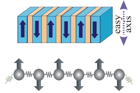
Figure 1: (Color online) Sketch of an antiferromagnetically coupled multilayer corresponding one-dimensional spin chain. The ”exchange springs” are cut at the ends of the finite chain.

As was mentioned above the basic model for two antiferromagnetically coupled layers is equivalent to the classical mean-field description of two-sublattice bulk antiferromagnets. Turov65 ; Stryjewski77 These systems compose two large groups: antiferromagnets with weak anisotropy Turov65 and strongly anisotropic uniaxial crystals that are commonly called metamagnets.Stryjewski77 The metamagnetic phase transition between the antiferromagnetic and ferromagnetic phases has been observed and investigated in many antiferromagnetic bulk systems.Stryjewski77 Easy-axis antiferromagnets with weak anisotropy also compose a large group of magnetically ordered crystals. For bulk antiferromagnets, the spin-flop transition has been predicted by Néel Neel36 and later was observed experimentally in CuCl${{}_{2}\cdot}$ 2H ₂O.Poulis52 In the next fifty years, spin flop transitions have been discovered and carefully studied in many classes of antiferromagnets (see bibliography in Refs. [Turov65, ; UFN88, ; PRB02, ]).

The interest in spin-flops revived with the synthesis of magnetic multilayer stacks with indirect antiferromagnetic exchange coupling through spacers.Wang94 These artificial antiferromagnetic layers, with few magnetic units as macroscopic spins instead of atomic spins (Fig. 1) offer the possibility to study field-driven reorientation transitions with unusually low exchange compared to anisotropies.Mills99 Experimental investigations in Fe/Cr(211) antiferromagnetic superlattices Wang94 seemed to confirm the scenario of the surface spin-flop transition introduced in Refs. [Mills68, ; Keffer73, ]. The observation was supported by numerical investigation of an elementary micromagnetic model.Wang94 ; Wang94b But, investigations on the magnetism of such antiferromagnetic superlattices and thin films did not produce a consistent understanding of the occurrence and nature of “spin-flop” transitions or other reorientation transitions in layered antiferromagnetic structures. Recent experiments demonstrate complex behaviour and different scenarios for the evolution of the magnetic states. Howson94 ; Zabel94 ; Zabel96 ; Fullerton97 ; Chesman98 ; Bab98 ; Hilt99 ; Temst00 ; Fitzsimmons00 ; Nolting00 ; Vavassori01 ; Felcher02 ; Lauter02 ; Nagy02 ; Aliev02 ; Lauter03 The problem of the magnetic states in antiferromagnetic superlattices with uniaxial anisotropy is strongly related to the long standing problem of a “surface spin-flop” discussed in various papers. Vernon78 ; Luthi83 ; Barron87 ; Lepage90 ; Wang94 ; Trallori94 ; Trallori95 ; Wang94b ; Stamps94 ; Micheletti97 ; Chung97 ; Rakhmanova98 ; Papan98 ; Momma98 ; Zhedanov98 ; Mills99 ; Dantas99 ; Papan99 ; Papan00 Theoretical investigations are mostly based on numerical calculations within a certain model, here called Mills model. Trallori94 ; Trallori95 ; Chung97 ; Rakhmanova98 ; Papan98 ; Momma98 Further theoretical works related these finite or semi-infinite antiferromagnetic chain models to systems like the Frenkel-Kontorova model.Micheletti97 ; Trallori98 These studies have led to controversial results and generated a long-drawn discussion about the physical nature of the reorientation transformations in the antiferromagnetic superlattices. Trallori94 ; Chung97 ; Micheletti97 ; Rakhmanova98 ; PRB03 ; PRB04 Only few attempts have been made to gain a complete understanding of the ground-state structure of the basic one-dimensional models for these superlattices.Micheletti97 ; Momma98 ; PRB04 Thus, the basic questions, whether, when, and how a surface spin-flop occurs, were unresolved.

A full set of solutions for the model under discussion was recently obtained by us.PRB04 These outwardly simple systems with few degrees of freedom own rich phase diagrams because of the competition between internal stiffness and anisotropy in conjunctions with restricted dimensionality. Present paper presents an extended account and an analysis of the solutions from Refs. [PRB04, ; pss04, ]. We explain the physical mechanism responsible for the formation of the main magnetic states in antiferromagnetic superlattices. We derive a clear and simple picture of the phenomena which have been discussed as “surface spin-flop”. We demonstrate the connections with bulk antiferromagnetic systems and other classes of magnetic nanostructures. PRB04a ; JMMM04

The structure of the paper is as follows: The phenomenological model and its variants are introduced in Sec. II. The analysis of possible magnetic states in the system starts from two limiting cases of low and high uniaxial anisotropy. The full solution for the generic highly symmetric Mills model in applied fields along the easy axis are presented in Sec. III and the general structure of the phase diagrams are presented. In this section, mainly analytical and numerical examples are employed to explain these solutions. Generalizations are briefly indicated. The methods can be extended to solve any other more general model for an antiferromagnetic multilayer system. In Sec. IV we exploit the fact that the models for low-anisotropy antiferromagnetic superlattices can be reduced to equivalent models for a chain of exchange coupled two-sublattice antiferromagnets. This dimerization transformation reveals the physical mechanisms ruling the magnetic states and reorientation transitions. Numerical results for the evolution of inhomogeneous spin-flop phases, magnetization curves, and phase diagrams are presented along with this discussion. In particular the limit of large numbers of layers and the emergence of the bulk spin-flop for such finite systems are discussed. Then, the continuum representation of the general models is presented. This offers a different point of view for the weak anisotropy. This continuum approximation is applicable to any weakly anisotropic system. It allows to derive the structure of the inhomogeneous spin-flop phase for arbitrary models, in particular model where the magnetic moments at the surfaces are partially compensated. Hence, the succession of field-driven phase transitions between the antiferromagnetic state towards the saturated ferromagnetic state via this spin-flop phase can be completely analysed. In Sec. V.1 the general picture of magnetic states in antiferromagnetic nanostructures and some recent experimental results are discussed in the context of the new results.

II Model

II.1 The micromagnetic energy. Mills model

Let us consider a stack of $N$ ferromagnetic plates infinite in $x$- and $y$-directions and with finite thickness along the $z$-axis. The magnetization of each plate is $\mathbf{m}_{i}$, and they are antiferromagnetically coupled through spacers. Replacing this system by a chain of single-domain particles with spontaneous magnetization $m_{0}^{(i)}=|{\mathbf{m}}_{i}|$, we may describe the magnetic configuration by the variables ${\mathbf{s}}_{i}={\mathbf{m}}_{i}/m_{0}^{(i)}$, i.e., by the set of unity vectors along the magnetization of the $i$th layer. We assume that the ferromagnetic layers have a uniaxial magnetic anisotropy with a common easy axis. The phenomenological energy of this system can be written as

$${{\Theta}}_{N}=\sum_{i=1}^{N-1}\left[J_{i}\,\mathbf{s}_{i}\cdot\mathbf{s}_{i+1}+\widetilde{J}_{i}\,\left(\mathbf{s}_{i}\cdot\mathbf{s}_{i+1}\right)^{2}\right]-\mathbf{H}\cdot\sum_{i=1}^{N}\,\zeta_{i}\,\mathbf{s}_{i}$$

$$-\frac{1}{2}\sum_{i=1}^{N}K_{i}\left(\mathbf{s}_{i}\cdot\mathbf{n}\right)^{2}-\sum_{i=1}^{N-1}K^{\prime}_{i}\left(\mathbf{s}_{i}\cdot\mathbf{n}\right)\left(\mathbf{s}_{i+1}\cdot\mathbf{n}\right)+e_{a}(\mathbf{s}_{i})\,.$$ (1)

Here, $\zeta_{i}=m_{0}^{(i)}/m_{0}$ designate deviations of the magnetization in the $i$-th layer from the average value $m_{0}$. $J_{i}$ and $\tilde{J}_{i}$ are constants of bilinear and biquadratic exchange interactions, respectively. The unity vector $\mathbf{n}$ points along the uniaxial anisotropy direction; $K_{i}$ and $K^{\prime}_{i}$ are constants of the in-plane and inter-plane uniaxial anisotropy. Finally, $e_{a}(\mathbf{m}_{i})$ collects higher-order uniaxial and in-plane magnetic anisotropy contributions, e.g., intrinsic cubic (magnetocrystalline) anisotropy in systems like Fe and Ni layers.

The functional (1) generalizes similar models considered earlier in a number of studies on magnetic states in antiferromagnetic multilayers with uniaxial anisotropy. Wang94 ; Trallori94 ; Trallori95 ; Wang94b ; Stamps94 ; Micheletti97 ; Rakhmanova98 ; Papan98 ; Momma98 ; Zhedanov98 ; Dantas99 In a recent paper on antiferromagnetic superlattice with higher (tetragonal) symmetry, Ref. [PRB04a, ], we have discussed the general model and the justification of the approach used for this class of systems. Therefore, the reader is referred to PRB04a for a detailed discussion and further references. Eq. (1) comprises the magnetic energies due to the main physical mechanisms, which are present in magnetic multilayers with indirect exchange through spacer layers (see Fig. 1). The ferromagnetic layers can be considered as homogeneously magnetized blocks with constant values of the magnetic interactions. This assumption relies on the fact that in ferromagnetic nanolayers the intrinsic (direct) exchange coupling are usually very strong. Thus, they play the dominating role for the magnetic order within the layers which react also very stiffly on all external and induced magnetic forces. Thus, the internal magnetic structure of an individual layer experiences little change under influence of the induced magnetic forces at the surfaces and interfaces, and the reorientation of other layers in the stack. This hypothesis has been justified by successful applications of such models to describe magnetization processes in layered ferro- and antiferromagnetic nanostructures in different classes. Johnson96 ; Thiaville92 ; PRL01 ; Wang94 ; Zabel94 ; Ustinov01 ; Lauter02 ; PRB03

Antiferromagnetic multilayers with uniaxial anisotropy and in applied field along the axis $\mathbf{n}$ show the strongest reorientation effects. Here, we address the overall magnetic properties of such uniaxial systems. Their behaviour may be analysed by considering only terms with bilinear exchange $J$, uniaxial intralayer anisotropy $K$ and an external field $H$. The form of the energy in Eq. (1) considers additional terms, which are known to play a role in antiferromagnetically coupled multilayers. In particular, strong biquadratic exchange has been revealed in a number of antiferromagnetically coupled multilayers.Ruhrig91 ; Demokritov98 ; Chesman98 ; Ustinov01 In Ref. [PRB04a, ], we have studied the related phenomenological model for multilayers with zero and with four-fold (tetragonal) anisotropies and we have discussed the relevance of biquadratic exchange ($\widetilde{J}\neq 0$), which plays essentially only a quantitative role for the competition between the various possible magnetic states as long the antiferromagnetic ground-state remains collinear.

The uniaxial anisotropies may be intrinsic to the magnetic material of the film or induced by surface effects. Thus, the uniaxial anisotropies can be strongly changed with respect to bulk systems, and their strengths can be controlled in film system within wide margins. Combination with intrinsic and induced fourth-order anisotropy, as considered in $e_{a}$ in Eq. (1), may lead to peculiarities of magnetic properties, see Refs. [Zabel94, ; PRB04a, ], but here we will disregard these contributions. Finally, strong demagnetization effects in antiferromagnetic superlattices with perpendicular anisotropy are responsible for complex evolution of multidomain states and specific magnetization processes.Hellwig03 ; Itoh03 ; Hellwig03b ; JMMM04 ; Hellwig05 To investigate these effects the stray-field energy must be included in Eq. (1), and the corresponding magnetostatic problem has to be solved.

The magnetic superlattices with antiferromagnetic coupling can be separated into two classes: non-compensated systems with a net magnetization and those with fully compensated magnetization. In the former case, the net magnetic moment strongly determines their global magnetic properties. In many physical aspect their properties are similar to those of bulk ferrimagnets. The main subject of this paper are the multilayers with fully compensated magnetization,i.e., multilayers with even $N$ and equal magnetization in all layers are similar to bulk collinear antiferromagnets. For simplicity, we assume $\zeta_{i}=1$ in all layers $i=1\dots N$. At the end of the paper we also consider effects imposed by a partial compensation of the magnetization in the endmost layers, i.e., deviations of $\zeta_{1}$ and $\zeta_{N}$ from unity.

For the reorientation effects in the antiferromagnetically coupled chain (Fig. 1), the effect due to the cut exchange bonds at the surface dominates. The last moments in the chain are coupled only to one neighbour while “internal” moments interact with two. Thus, the moments at the surface experience a weakened exchange stiffness and are more susceptible to the reorienting influence of an applied field. Due to this cut exchange at the surfaces the boundary moments oriented against the external field turn into the field direction in lower fields than internal moments. The simplified version of the model (1) with equal constants $J_{i}=J$, $K_{i}=K$, and $\widetilde{J}_{i}=K^{\prime}_{i}=e_{a}=0$ for an applied field in direction of the easy axes, $\mathbf{H}\parallel\mathbf{n}$, describes the effect of the cut bonds as the sole surface-imposed factor. It allows to investigate this surface effect separately from other interactions.

Usually the magnetization of the layers is confined to a certain plane. For many multilayers, this is the film plane owing to demagnetization. For this case the deviations of $\mathbf{m}_{i}$ from the anisotropy axis can be described by angles $\theta_{i}$, and the energy (1) in the equal constant model is reduced to the following form

$$\Phi_{N} = J\sum_{i=1}^{N-1}\cos(\theta_{i}-\theta_{i+1})$$

$$-H\sum_{i=1}^{N}\cos\theta_{i}-\frac{K}{2}\sum_{i=1}^{N}\cos^{2}\theta_{i}\,.$$

For $J>0$ and $K>0$, the Eq. (II.1) describes antiferromagnetically coupled ferromagnetic layers with easy-axis anisotropy in an external field along the anisotropy axis. Energy (II.1) has been introduced by Mills for a semi-infinite chain ($N=\infty$).Mills68 Later this model (called here Mills model) has been intensively studied for finite and infinite $N$ Keffer73 ; Vernon78 ; Luthi83 ; Barron87 ; Lepage90 ; Wang94 ; Trallori94 ; Trallori95 ; Wang94b ; Stamps94 ; Micheletti97 ; Chung97 ; Rakhmanova98 ; Papan98 ; Momma98 ; Zhedanov98 ; Mills99 ; Dantas99 ; Papan99 ; Papan00 and has been used as basic ansatz to analyze experimental results in antiferromagnetically coupled multilayers. Wang94 ; Felcher02 ; Lauter03

Both the exchange interactions and uniaxial anisotropy in (II.1) have surface/interface induced nature, their values are very sensitive to many physical factors such as the structure of the spacers and substrates. Johnson96 ; Moriarty01 Hence, the materials parameters may vary from layer to layer in the stack. A generalization of the Mills model may include differing parameters for each layer

$$\widehat{\Phi}_{N} = \sum_{i=1}^{N-1}J_{i}\,\cos(\theta_{i}-\theta_{i+1})$$

$$-H\sum_{i=1}^{N}\zeta_{i}\,\cos(\theta_{i})-\frac{1}{2}\sum_{i=1}^{N}K_{i}\cos^{2}\theta_{i}\,.$$

This is a general model for antiferromagnetic multilayers. Even for a stack of identical nanolayers, the top and bottom layers still have a different “neighbourhood” than internal layers. To describe these effects we may introduce a modified Mills model with equal materials parameters for all internal layers $J_{i}=J$ ($i=2,3,$ … $,N-2$), $K_{i}=K$ ($i=2,3,$ … $,N-1$) and different values for the first and last layer ($J_{1}=J_{N-1}=J_{s}$, $K_{1}=K_{N}=K_{s}$, $\zeta_{1}=\zeta_{N}=\zeta_{s}<1$)

$$\widetilde{\Phi}_{N} = J_{s}\left[\cos(\theta_{1}-\theta_{2})+\cos(\theta_{N-1}-\theta_{N}\right]$$

$$+J\sum_{i=2}^{N-2}\cos(\theta_{i}-\theta_{i+1})$$

$$-H\zeta_{s}\left(\cos\theta_{1}+\cos\theta_{N}\right)-H\sum_{i=2}^{N-1}\cos\theta_{i}$$

$$-\frac{1}{2}K_{s}\left(\cos^{2}\theta_{1}+\cos^{2}\theta_{N}\right)-\frac{K}{2}\sum_{i=2}^{N-1}\cos^{2}\theta_{i}\,.$$

In all these cases, calculations of the magnetic states for the antiferromagnetic superlattices can be reduced to the minimization of the energy functions $\Phi_{N}(\theta_{1},\theta_{2},\,\dots\,,\theta_{N})$. In this paper, we study in detail solutions for the chains with equal constants as described by Mills model (II.1), and we discuss the generalizations according to Eqs. (II.1) and (II.1).

II.2 General features of the solutions. Relation to bulk antiferromagnetism

The antiferromagnetic multilayers with $N=2$ are of particular importance for investigations on surface/interface-induced interactions. Zabel94 ; Chesman98 ; Bab98 ; Vavassori01 In experimental works they are often referred as “trilayers”, we use here the term “two-layer systems”. The energy (II.1) for $N=2$ is the same function as the mean-field magnetic energy of a bulk two-sublattice antiferromagnet

$$\widetilde{\Phi}_{2} = J\,\mathbf{s}_{1}\cdot\mathbf{s}_{2}-H\,[\left(\mathbf{s}_{1}\cdot\mathbf{n}\right)+\left(\mathbf{s}_{2}\cdot\mathbf{n}\right)]$$ (5)

$$-\frac{K}{2}\left[\left(\mathbf{s}_{1}\cdot\mathbf{n}\right)^{2}+\left(\mathbf{s}_{2}\cdot\mathbf{n}\right)^{2}\right]\,.$$

We briefly review the reorientation transitions in these two-layers systems to fix our notation and terminology. Following a general convention we introduce the linear combinations of the magnetization vectors $\mathbf{s}_{1,2}=\mathbf{M}\pm\mathbf{L}$, the total or net magnetization $\mathbf{M}$ and the staggered magnetization $\mathbf{L}$, that is also called vector of antiferromagnetic order Turov65 . The equations $|\mathbf{s}_{i}|=1$ lead to the constraints $\mathbf{M}^{2}+\mathbf{L}^{2}=1$ and $(\mathbf{M}\cdot\mathbf{L})=0$. In a magnetic field along the easy axis the vectors $\mathbf{H}$, $\mathbf{s}_{1}$ and $\mathbf{s}_{2}$ lie in a fixed plane. The magnitude of the net magnetization $M=|\mathbf{M}|$ can be used as an internal parameter. After an independent minimization with respect to $M$, the energy and the net magnetization depend only on the orientation of the staggered vector $\mathbf{L}$ and can be expressed as functions of the angle $\phi$ between anisotropy axis $\mathbf{n}$ and $\mathbf{L}$

$$\widetilde{\Phi}_{2}(\phi) = -\frac{H^{2}\sin^{2}\phi}{(2J+K\cos 2\phi)}-K\cos^{2}\phi+J,$$ (6)

$$M = \frac{2H\sin\phi}{(2J+K\cos 2\phi)}\,.$$ (7)

Then, the phase diagram of the antiferromagnetic two-layer system is given by the potential energy for a system with one variable $\phi$ (7) with the control of materials parameters $K/J,H/J$. This phase diagram is plotted in Fig. 2. The structure of the phase diagram is determined by the following characteristic fields

$$H_{\mathrm{tr}}=\sqrt{K(2J-K)},\;H_{\mathrm{FM}}=J,\;H_{\mathrm{F}}=(2J-K)$$

$$H_{\mathrm{AF}}=\sqrt{K(2J+K)},\;H_{\mathrm{SF}}=(2J-K)\sqrt{\frac{K}{2J+K}}\,.$$ (8)

For $K<J$ a first-order transition between the antiferromagnetic (AF) phase with $\phi=0,\pi$ and the spin-flop phase (SF) with $\phi=\pm\pi/2$ occurs at the spin-flop field $H_{\mathrm{tr}}$. The fields $H_{\mathrm{AF}}$, $H_{\mathrm{SF}}$ are stability limits of these two competing phases. The difference $H_{\mathrm{AF}}-H_{\mathrm{SF}}$ gives the width of the metastability region. Because the antiferromagnetic state has zero magnetization the magnetization jump at the first-order transition, $\Delta M=m_{0}\,M_{\mathrm{SF}}(H_{\mathrm{tr}})=m_{0}\,\sqrt{K/(2J-K)}$ exactly in the field $H_{\mathrm{tr}}$, equals the magnetization of the spin-flop phase. For increasing anisotropy $K$ this magnetization jump $M_{\mathrm{SF}}(H_{\mathrm{SF}})$ gradually increases from very small values $M\ll 1$ for $K\ll J$ to the saturation value $M=1$ which marks the end point of the first-order transition line between the AF and SF phase that is reached at $K=J$. A continuous transition from the SF phase to the ferromagnetic (F) phase occurs at $H_{\mathrm{F}}$. This transition leading to an enforced field-polarized state is usually referred to as spin-flip transition.

For $K>J$, the SF phase does not arise as a stable state; instead there is a direct first-order transition between the AF and F phase at $H_{1}=J$. Such transitions in antiferromagnets are known as metamagnetic transition.Stryjewski77 For this high anisotropy region, $K>J$, the critical field $H_{\mathrm{F}}$ plays the role of the stability limit for the ferromagnetic phase (Fig. 2). The metamagnetic transition is characterized by a large jump of the magnetization $\Delta M(H_{1})=m_{0}$ and extremely broad metastability regions.

For low-anisotropy systems in the region $K\ll J$, the energy (7) can be simplified

$$\widetilde{\Phi}_{2}(\phi)=\left(\frac{H^{2}-H_{0}^{2}}{4J}\right)\cos 2\phi,\qquad H_{0}=\sqrt{2JK}\,.$$ (9)

In this limit the metastable region is restricted to a close vicinity of the spin-flop field: $H_{\mathrm{AF}}\approx H_{\mathrm{SF}}\approx H_{\mathrm{tr}}\approx H_{0}$. This simplified potential energy Eq. (9) reveals the physical mechanism of the spin-flop transition. At zero field the uniaxial anisotropy stabilizes the antiferromagnetic phase. The potential wells at $\phi=0,\pi$ corresponding to the two antiferromagnetic states are stable. An increasing applied field, $H<H_{\mathrm{tr}}$, gradually reduces the height of the potential barrier between the antiferromagnetic states. At the threshold spin-flop field $H_{\mathrm{tr}}$ the stable potential wells switch into the configurations $\phi=-\pi/2$, $\phi=\pi/2$ that correspond to the flopped states (Fig. 2).

Contrary to natural antiferromagnetic crystals which are described only by marginal parts of the $K/J$ scale with either low anisotropy, $K/J\ll 1$, or very large anisotropy, $K\gg 1$, antiferromagnets composed of magnetic nanolayers can have arbitrary values of $K/J$. These artificial antiferromagnets cover the whole phase plane in Fig. 2.

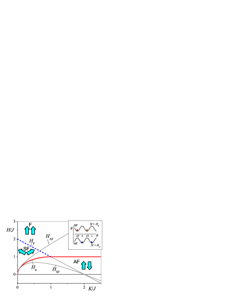
Figure 2: (Color online) The phase diagram of the solutions for a two-layer system includes antiferromagnetic (AF), spin-flop(SF) and ferromagnetic (F) phases. The AF phase is separated from the SF and F phases by the first-order transition lines (thick). The second-order “spin-flip” line $H_{\mathrm{F}}$ (dashed) separates SF and and F phases. Thin lines indicate stability limits of the corresponding phases. Inset: in the spin-flop field $H=H_{\mathrm{tr}}$ the potential wells switch from ($0$, $\pi$) (AF phase) to ($-\pi/2$, $\pi/2$) (SF phase).

In finite multilayers with $N>2$ the cutting of the exchange bonds at the surfaces (Fig. 1) causes a strong disbalance of the exchange interactions along the chain. This disbalance is the determining factor for the appearance of magnetic states in the system. The detailed analysis of the solutions for Mills model will be given in the next section. Here, we summarize the physical mechanism ruling the formation of magnetic configurations in simple terms. In the antiferromagnetic configuration the moments at one surface always point against an applied field. These moments can be reversed more easily than the internal moments because of the cut exchange. Depending on the relative strength of the exchange and anisotropy, this specific instability leads to different reoriented configurations. At very strong uniaxial anisotropy ($K\gg J$) the exchange coupling between layers becomes negligible. In this case the reorientation of the magnetization in the endmost layer does not influence magnetic states in the other layers. In an increasing field, a collinear spin configuration with an inverted endmost moment is reached. The corresponding ferrimagnetic (FM) phase becomes energetically stable at a field $H_{\mathrm{FM}}=J$ through a discontinuous first-order transition (Fig. 3). PRB04 ; JMMM04 In the opposite case of weak anisotropy, $K\ll J$, the exchange coupling plays the dominating role. Accordingly the overturn of the endmost moment is spread over the entire stack and creates a spatially inhomogeneous spin configuration (Fig. 3). PRB04 ; PRB04a In Ref. [PRB04, ] this mode was called inhomogeneous spin-flop phase. In increasing fields, a curious evolution takes place within this spin-flop phase, where some moments rotate against the applied field and change their sense of rotation at higher fields.PRB04a A continuous spin-flip into the saturated state occurs at an “exchange” field $H_{\mathrm{E}}$, which depends on the number of layers and on the anisotropy $K$. In the region of moderate anisotropy spatially inhomogeneous asymmetric states exist as transitional phases between the inhomogeneous SF and FM phases. These asymmetric phases arise by canting transitions, i.e., elastic distortions of the collinear FM phases when $K/J\stackrel{{\scriptstyle<}}{{{\sim}}}1$. These asymmetric canted (C) phases can be considered as superpositions of ferrimagnetic states and the inhomogeneous spin-flop state (Fig. 3). This means that in these low symmetry intermediate C phases all the symmetries are broken that are broken in the corresponding SF and FM phases. Thus, magnetic states arising in Mills model comprise antiferromagnetic, spin-flop, and ferromagnetic phases, which exist in bulk antiferromagnets, and additional ferrimagnetic and canted configurations. The latter phases are imposed by the exchange cut. They are specific to finite antiferromagnetic layer systems. In particular, the detailed solutions for larger $N$ show series of different canted phases. The corresponding phase diagrams include a large number of critical points and a tangled net of transition and lability lines (see examples in [Momma98, ; PRB04, ; pss04, ]). The cut exchange bonds underly this complexity as the general physical mechanism for the formation of the various inhomogeneous magnetic states and their transitions into the simple collinear states in the limiting regions of the phase diagram for and low high anisotropy and for large fields. Therefore, all these phase diagrams have a general topology represented in Fig. 3.

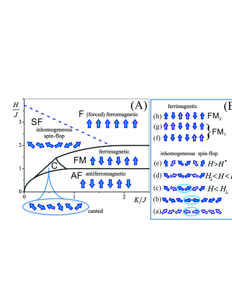
Figure 3: (Color online) Sketch of the phase diagram for $N=6$ introduces the main types of the solutions for Mills model Eq. (II.1) with arbitrary even $N$ (A). Due to the cut exchange bonds the flopped states are spatially inhomogeneous and can exist as symmetric inhomogeneous spin-flop phase (SF) for low anisotropy, or as asymmetric canted phases (C) for moderate anisotropies. In strongly anisotropic systems ($K\geq J$) spin configurations with flipped spins exist These collinear ferrimagnetic (FM) phases exist at intermediate fields between the antiferromagnetic and ferromagnetic states. The spin configurations in panel (B) show for $N=8$ the degeneracy of the inhomogeneous SF state for $N=8$ (a) and (b); for $N=6$ the evolution of the inhomogeneous SF in increasing field (c) to (e) and the two different types of FM states, where FM₁ is degenerate (f), (h) and FM₂ (h) is a collinear version of the inhomogeneous SF state (c)-(e) in an even-odd system.

III Phase diagram of the solutions

In this section we analyse the solutions for Mills model (II.1), derive the regions of their existence, and conditions of the transitions between different phases.

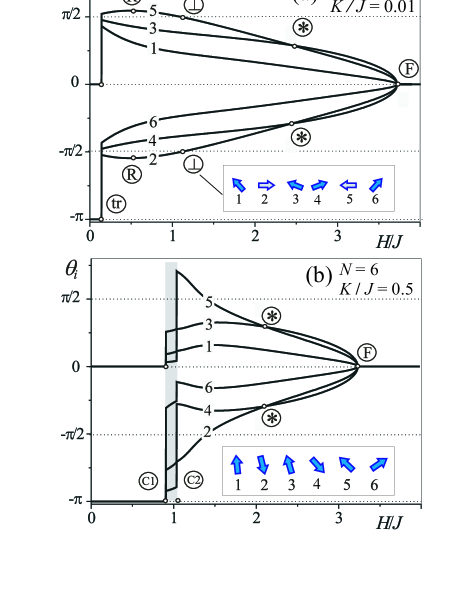
Figure 4: (Color online) Evolution of the equilibrium magnetic configurations $\theta_{i}$ in Mills model for antiferromagnetic $N=6$ layers with finite uniaxial anisotropy, $K=0.01\,J$ (a), $K=0.5\,J$ (b), in magnetic fields applied in direction of the easy axis. For the low anisotropy case only AF, SF, and F states exist (a). The points indicate the spin-flop field $H_{\mathrm{tr}}$ and the spin flip field $H_{\mathrm{F}}$. Characteristic fields are $H_{\mathrm{R}}$, $H_{\bot}$, and $H^{*}$ as marked in the plot. The spin configurations correspond to $H=H_{\bot}=1.104\,J$ where the magnetization in the 2th and 5th layer is perpendicular to the applied field. For intermediate anisotropy (b) canted asymmetric states exist in the field interval $H_{\mathrm{C1}}<H<H_{\mathrm{C2}}$. The spin configuration in (b) corresponds to the canted phase at the transition field $H_{\mathrm{C1}}=0.906\,J$.

III.1 Spin-flop transition and solutions for inhomogeneous spin-flop phases

We start with low-anisotropy systems ($J\gg K$). Here, we consider generalized models that keep mirror symmetry about the multilayer center with parameters $J_{i}=J_{N-i}$, $K_{i}=K_{N+1-i}$, etc., for $i=1\dots N-2$ or $N-1$, respectively. Then, the equations, that minimize the energy of these systems, have solutions for an inhomogeneous spin-flop phase with the property $\theta_{i}=-\theta_{N-i+1}$.PRB04 ; PRB04a These magnetic configurations have different properties when $N=4\,l$, i.e., $N$ is divisible by four called here even-even systems, or when $N=4\,l+2$ for even-odd systems ($l=1,2...$).

In low fields, ${J_{i}\gg H}$, the spins in the flopped state deviate only slightly from the the direction perpendicular to the easy axis

$$\theta_{2j-1}=\pi/2-\alpha_{2j-1},\;\theta_{2j}=-\pi/2+\alpha_{N-2j+1},$$ (10)

$$|\alpha_{2j-1}|\ll 1\qquad j=1,\dots N/2\,.$$

The expansion of energy (1) with respect to the small parameters $\alpha_{2j-1}$ allows to derive analytical solutions for the flopped states that can be formulated for arbitrary models. As an illustration we write the parameters $\alpha_{2j-1}$ for Mills model (II.1), i.e., with equal constants in the even-even case $N=8$

$$\alpha_{1}=\frac{2H}{J}\left(1+\frac{11}{2}\frac{K}{J}\right),\;\alpha_{3}=\frac{H}{J}\left(1+\frac{6K}{J}\right),$$ (11)

$$\alpha_{5}=\frac{2H}{J}\frac{K}{J},\;\alpha_{7}=\frac{H}{J}\left(1+\frac{9K}{J}\right),$$

and in the even-odd case $N=10$

$$\alpha_{1}=\frac{5}{2}\frac{H}{J}\left(1+\frac{17}{2}\frac{K}{J}\right),\;\alpha_{3}=\frac{3}{2}\frac{H}{J}\left(1+\frac{59}{6}\frac{K}{J}\right),$$

$$\alpha_{5}=\frac{1}{2}\frac{H}{J}\left(1+\frac{13}{2}\frac{K}{J}\right),\alpha_{7}=\frac{1}{2}\frac{H}{J}\left(1+\frac{37}{2}\frac{K}{J}\right),$$

$$\alpha_{9}=\frac{3}{2}\frac{H}{J}\left(1+\frac{25}{2}\frac{K}{J}\right)\,.$$ (12)

The Eqs. (10), (11), and (III.1) display the generic structure of these solutions which apply also for generalized models with arbitrary parameters. The deviations of the magnetization direction from the directions $\pm\pi/2$ are small of the order $H/J$. The corrections due to the anisotropy are of the order $(HK)/J^{2}$. The deviations of the magnetization direction in the different layers gradually increase towards the endmost layers $i=1$ or $i=N$, respectively. The dominating exchange interactions favour antiparallel ordering in the adjacent layers. In the flopped configurations (11), (III.1) pairs of spins essentially remain antiparallel. E.g., for $N=8$, the interior pairs $\mathbf{s}_{2}$, $\mathbf{s}_{3}$ and $\mathbf{s}_{6}$, $\mathbf{s}_{7}$ are almost antiparallel (Fig. 3 B, panel (a)). This fact may be stated more precisely. According to (11) $|\theta_{3}-\theta_{2}|=|\theta_{7}-\theta_{6}|=\pi-(3HK)/J^{2}$, this means the slight deviations from antiparallel arrangement are due to a second order effect. The exchange coupling in such pairs is stronger than the Zeeman energy of the pair. This causes an interesting effect, a reverse rotation of the magnetization in a number of layers. In the multilayer with $N=8$, the magnetizations $\mathbf{s}_{2}$, $\mathbf{s}_{7}$ undergo such a reverse rotation according to Eqs. (11); for the case $N=10$ the corresponding magnetizations are $\mathbf{s}_{2}$, $\mathbf{s}_{4}$, $\mathbf{s}_{7}$, and $\mathbf{s}_{9}$, see Eqs. (III.1).

For even-odd systems, the projections of the magnetization vectors for the central layers ($\mathbf{s}_{N/2}$, $\mathbf{s}_{N/2+1}$) onto the field direction are of the order $~{}H/J$, which is much larger than the corresponding projections of the order $~{}(HK)/J^{2}$ in even-even systems (compare solutions for $\theta_{4},\theta_{5}$ in Eqs. (11), $\theta_{5},\theta_{6}$ (III.1) and spin configurations in panels (a) and (c) Inset B of Fig. 3, respectively). The solutions $\theta_{i}(H)$ for Mills model of a multilayer with $N=6$ in Fig. 4 illustrate the general features of the field induced evolution of the spin-flop state. (See also the configurations in panels (c)-(e) in Inset B of Fig. 3, and the solutions for $N=16$ in Ref. [PRB04, ] and $N=12$ in Ref. [pss04, ]). An increasing magnetic field gradually slows down the reverse rotation of the spins with negative projections onto the field direction. Finally at characteristic fields $H_{R}^{(i)}$ the sense of rotation changes. In this point $d\theta_{i}/dH=0$. Another set of characteristic fields $H_{\bot}^{(i)}$ defines the points where the projection of $\mathbf{s}_{i}$ changes the sign, i.e., $(\mathbf{s}_{i}(H_{\bot}^{(i)})\cdot\mathbf{H})=0$. In an increasing field these characteristic fields, $H_{R}^{(i)}$ and then $H_{\bot}^{(i)}$, are reached first for the central layers and at higher fields for those closer to the boundaries. Fig. 4 (a) displays angles $\theta_{i}$ for an example of Mills model Eq. (II.1). with low $K\neq 0$. Finally, for Mills model at a particular field $H^{\star}$ the projection of the magnetization onto the field direction is equal for all interior layers. This knot point is designated by “$\star$”. The value of $H^{\star}$ is analytically given by

$$H^{\star} = 2\sqrt{3}J\left(1-\frac{K}{4J}\right)\left(1+\frac{K}{3J}\right)^{1/2}\times$$

$$\times\left[1+\frac{3K}{4J}+\sqrt{1+\left(\frac{K}{4J}\right)^{2}\,}\;\right]^{-1/2}\,.$$

In particular, for $K=0$ the knot point is $H^{\star}=\sqrt{6}\,H_{\mathrm{F}}/4$, which coincides with the value derived in Ref. [PRB04a, ]. For $H>H^{\star}$ the positive projections of the magnetization onto the direction of the magnetic field decreases towards the center. The inhomogeneous spin-flop states for isotropic Mills models, $K\equiv 0$, exist starting from zero field and have similar features as those for finite anisotropy. PRB04a

III.2 Critical lines and multicritical points

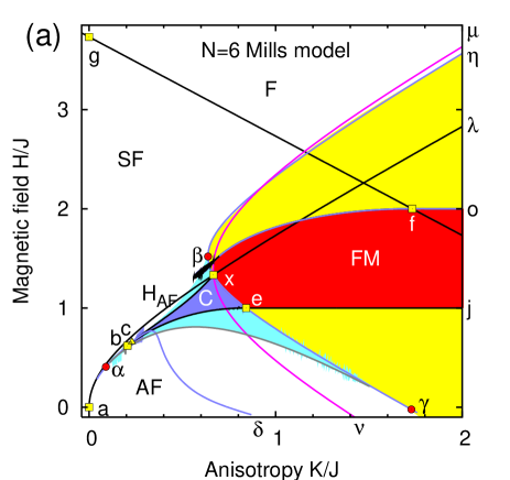
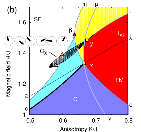
Figure 5: (Color online) Phase diagram for Mills model with $N$=6 (a). Detail of phase diagram for Mills model with $N$=6 (b). Special canted states C_X (sketched configuration) are stable in the hatched area. The point $y$ is a triple point, where FM, SF, and C_X phase coexist. Triangles designate tricritical points, where the SF-C_X transitions change from continuous to first-order with increasing anisotropy.

In this section we determine stability regions of the solutions, conditions of the phase transitions between them and construct the phase diagrams. Mills model (II.1) has three independent control parameters $K/J$, $H/J$, and $N$. Correspondingly a set of ($K/J,\,H/J$) phase planes for different $N$ provides complete information about the solutions for the model (II.1). As illustration we present the ($K/J,\,H/J$) phase diagram for Mills model with $N=6$ (Fig. 5), which containts all essential features of the generic phase diagram and some complications (Fig. 5(b)), which are absent in the simplest case $N=4$ as presented in Ref. [PRB04, ]. The essential critical points for Mills models with $N=4\dots 16$ are given in Table I. Then we proceed to discuss general features of the model with arbitrary $N$.

To determine the conditions for the phase transitions between different spin configurations and the stability regions of these phases we may use standard procedures. The equality of the equilibrium energies of the competing phases yields the condition of the first-order transitions. The stability of the solutions $\{\theta_{i}\}_{i=1,\dots,N}$ can be checked by writing the energy of the system for small arbitrary distortions, $\tilde{\theta}_{i}=\theta_{i}+\delta\theta_{i}$, which yields the expansion

$$\Phi_{N}(\tilde{\theta}_{i}) = \Phi_{N}(\theta_{i})+\sum_{i,j=1}^{N}A_{ij}\delta\theta_{i}\delta\theta_{j},$$

$$A_{ij}=\partial^{2}\Phi_{N}/\partial\theta_{i}\partial\theta_{j}\,.$$

The solutions $\theta_{i}$ are stable, if all eigenvalue of the symmetric matrix $\mathbf{A}_{N}=((A_{ij}))$ are positive. In particular, for the AF phase within Mills model the matrix $\mathbf{A}_{N}$ has a band structure given by $A_{2j-1,\,2j-1}=J+K+H$, $A_{2j,\,2j}=J+K-H$ for $j=1\dots N/2$, and $A_{i,\,i+1}=A_{i+1,\,i}=J$ for $j=1\dots N-1$. All other elements are equal zero. The determinant $D_{N}=\det(\mathbf{A}_{N})$ can be reduced to the following form

$$D_{N} = \underbrace{[H^{2}-H_{\mathrm{AF}}^{2}]}_{D_{2}}\times$$

$$\times\{[H^{2}-(K^{2}+4JK+2J^{2})]D_{N-4}$$

$$+[H^{2}-(K^{2}+4JK+3J^{2})]\sum_{i=3}^{N/2}(-1)^{i}D_{N-2i}\}\,.$$

The obvious convention $D_{0}=1$ and $D_{k}=0$ for $k<0$ starts the recursion in Eq. (III.2). Any determinant $D_{N}$ includes the determinant $D_{2}$ for a two-layer system $D_{2}$ as a multiplier. Thus, within the Mills model (II.1) the lability field of the AF phase has the same value for arbitrary values of $N$ Keffer73 ; Micheletti97 ; Zhedanov98 ; Dantas99 . It coincides with that for a bulk antiferromagnet $H_{\mathrm{AF}}=\sqrt{K\,(2J+K)}$ (8).

Note that this simple result for the stability limit of the AF phase holds only for Mills model because of its high symmetry. For general models (see Eq. (III.2)), $H_{\mathrm{AF}}$ is an involved combination of the materials parameters and depends on $N$. For example, for the modified Mills model one derives

$$D_{N} = \left(H^{4}+p_{1}H^{2}+q_{1}\right)D_{N-4}$$

$$+\left(H^{4}+p_{2}H^{2}+q_{2}\right)\sum_{i=3}^{N/2}(-1)^{i}D_{N-2i}\,,$$

where $p_{1}=3J^{2}-(J+K)^{2}-(J_{s}+K_{s})^{2}$, $p_{2}=p_{1}-J^{2}$, $q_{1}=q_{0}-J^{2}(J_{s}+K_{s})^{2}$, $q_{2}=q_{0}-J^{4}$, and $q_{0}=[J^{2}-(J+K)(J_{s}+k_{s})]^{2}$. The determinants $D_{N-2j}$ ($j>2$) in the right part of Eq. (III.2) are sub-determinants and do not include “surface” terms.

In Fig. 6 the low-anisotropy region is shown by $\Delta H$–$K$-phase diagrams for $N$=6 as representative for the general behaviour. Here, magnetic fields are given relative to $H_{\mathrm{AF}}$, i.e. $\Delta H\equiv H-H_{\mathrm{AF}}$. The stability limit for the antiferromagnetic phase is always above the lower stability limits of the symmetric and inhomogeneous SF-phase.

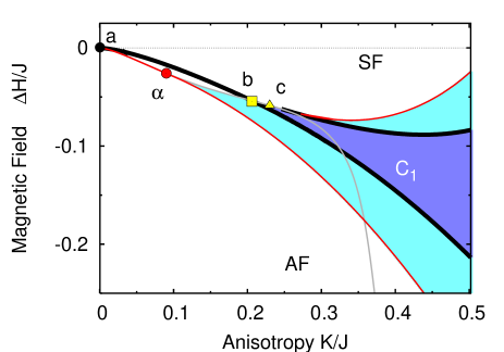
Figure 6: (Color online) Low anisotropy region of the phase diagram for Mills model with $N$ = 6. The magnetic field is given relative to the stability limit of the AF phase by $\Delta H=H-H_{\mathrm{AF}}(K)$. The canted phase C₁ is stable in the darker (blue) area. It is metastable in the brighter (turquoise) areas. Thick black lines give the first-order spin-flop transition from AF to SF and AF to C, respectively. For anisotropies below point $\alpha$ only a first-order spin-flop from AF to the symmetric SF-phase exists. At higher anisotropies above the point $b$, the first-order transition is from SF to the asymmetric canted C-phase. For $K_{\alpha}<K<K_{b}$, the canted phase exists only as a metastable state. For $K>K_{c}$ above the tricritical point $c$, the transition from the asymmetric phase C₁ to the spin-flop phase is first-order. Line $a$-$\alpha$-$b$ is the lower stability limit of the AF-phase, along the line $\alpha$-$b$-$c$ the continuous transition between C and SF takes place. Lines starting at point $\alpha$ are the metastability limits of the canted phase C.

Comparing the equilibrium energies in the AF and SF phase we determine the field for the first-order transition between these two phases (Fig. 6). In the low-anisotropy limit this first-order transition line and the two lability fields for the stability limits of the AF and SF phase, respectively, are close to the value $H_{0}=\sqrt{2\,JH\,}$ from Eq. (9). The difference between them defining the co-existence region for metastable states is of order $H_{0}(K/J)\ll H_{0}$.

Figure 7: Hysteresis for Mills model $N=6$ and an anisotropy value, where a canting instability of the spin-flop phase occurs in the metastability region $K_{\alpha}<K<K_{b}$. A resulting magnetic configuration of the canted C₁-state is shown. Field $H_{\mathrm{tr}}$ for the first-order transition between antiferromagnetic and spin-flop-phase, and upper stability limit $H_{\mathrm{AF}}$ of the antiferromagnetic phase are indicated.

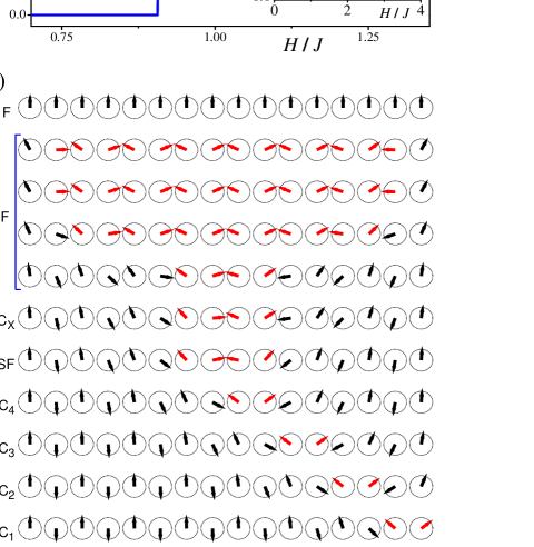
Figure 8: (Color online) Equilibrium solutions for Mills model with $N$=16 and intermediate anisotropy $K/J=0.5$. In increasing field a series of transition lead from antiferromagnetic to ferromagnetic phase via several canted (C_i) and (reentrant) spin-flop states. Left panel: magnetization of the equilibrium states(first-order transitions are marked by arrows). Right panel: spin-configurations in the canted in spin-flop states.

Near the spin-flip transition from the SF to the F phase, the deviations of $\mathbf{s}_{i}$ from the field directions are small ($\theta_{i}\ll 1$), and for model Eq. (II.1) the stability matrix in Eq. (III.2) becomes $\Phi_{N}(\tilde{\theta}_{i})=\sum_{i,j=1}^{N}A_{ij}\theta_{i}\theta_{j}$ with $A_{ij}$ having a tridiagonal band matrix form where nonzero elements occur only in the main diagonal and the first side diagonals. In particular, for Mills model $A_{ii}=H+K-J$, $A_{i,\,i-1}=A_{i-1,\,i}=J$, and the spin-flip or exchange field is a linear function of $K$

$$H_{\mathrm{E}}^{(N)}(K)=2J+K_{f}-K,\quad H_{\mathrm{E}}^{(N)}(0)=2J+K_{f}\,,$$ (17)

where $K_{f}$ is defined as the value of uniaxial anisotropy in the point $f$ where, depending on $N$, the line $H_{\mathrm{E}}^{(N)}(K)$ intersects line $H_{\mathrm{FM}}=2\,J$. The line $H_{\mathrm{FM}}$ is the transition line between the ferromagnetic and ferrimagnetic phases. The value $K_{f}$ can be derived analytically as solutions of the equation $D_{N}(A_{ij})=0$ with $A_{ii}=K_{f}-J$, $A_{i,\,i-1}=A_{i-1,\,i}=J$ ( Table I); $H_{\mathrm{E}}^{(N)}(0)=2J+K_{f}$ is the spin-flip field for zero anisotropy (in point $g$, Fig. 5). In Ref. [PRB04a, ] the spin-flip fields have been calculated for generalized isotropic models including biquadratic exchange.

For systems with larger anisotropies, an asymmetric canted phase C₁ occurs first as a metastable state for $K_{\alpha}<K<K_{b}$, which can be reached by a continuous canting of the spin-flop phase. A corresponding hysteresis around the first-order transition between AF and SF-phase is shown in Fig. (7) with an example of the magnetic configuration C₁. This canted phase C₁ is derived from elastically distorting the collinear ferrimagnetic state FM₁ with a ferromagnetically aligned pair at the surface. For even larger anisotropy $K_{b}<K$, the C₁ state becomes a stable phase of the system, which is reached from the AF-state through a first-order transition. In the $H$ vs. $K$-phase diagrams, the magnetic fields for the upper and lower stability limit of the canted phase C₁ meet at the critical point $\alpha$ at ($K_{\alpha}$, $H_{\alpha}$) This point also delimits the line for the canting instability of the metastable SF-state. The critical line for the canting instability of the stable SF-state ends in the critical point ($K_{b}$, $H_{b}$) on the line of first-order transitions $H_{\mathrm{tr}}$ between either the AF-phase and the SF-phase below $K_{b}$, or the AF-phase and the C₁-phase above $K_{b}$. This point $b$ located at ($K_{b}$, $H_{b}$) designates the lower anisotropy limit, where the phase C₁ and any asymmetric canted phase is stable for Mills models. The topology of the phase diagrams in Fig. 6 for the corner of low anisotropy $K<K_{\alpha}$ and fields describes the general behaviour for arbitrary $N$. From our previous analysis, we have seen that no canted asymmetric phase may occur at low anisotropies. The first canting instability at higher anisotropy will occur into a phase similar to the C₁ phase with a flopped configuration at the surface. For Mills models with various $N$ we have numerically determined the low-anisotropy parts of the phase diagrams and verified this general topology. Coordinates of the two critical points $\alpha$ and $b$ for the canting instabilities are collected in Table 1. from numerical investigations of Mills models with $N=4,6,..,16$.

Magnetization curves corresponding to the equilibrium states, where the canted state C₁ is a stable phase are shown in Fig. 7. For anisotropy $K>K_{b}$ further transitions and critical points occur depending on $N$. E.g., the transition between the C₁-phase and the spin-flop for $N=6$ becomes first-order above a tricritical point $c$.

Table 1: List of main critical points in the field-anisotropy phase diagrams for Mills model antiferromagnetic multilayers with $N=2,4,\dots,16$. Field and anisotropy values are given in units of $J$.

$N$	($K_{\alpha}$, $H_{\alpha}$)	($K_{b}$, $H_{b}$)	($K_{\beta}$, $H_{\beta}$)	$K_{e}$	$K_{f}$
4	(0.160, 0.522)	(0.300, 0.730)	(0.622102, 1.57956)	0.847759	21/2
6	(0.090, 0.408)	(0.206, 0.620)	(0.637223, 1.51922)	0.842236	31/2
8	(0.051, 0.312)	(0.120, 0.481)	(0.639260, 1.50798)	0.842001	$\sqrt{2+2^{1/2}}$
10	(0.034, 0.256)	(0.080, 0.394)	(0.639621, 1.50545)	0.8419914	$\sqrt{10+20^{1/2}}/2$
12	(0.024, 0.217)	(0.056, 0.332)	(0.639689, 1.50486)	0.841990990	$(6^{1/2}+2^{1/2})/2$
14	(0.019, 0.193)	(0.042, 0.286)	(0.639702, 1.50472)	0.8419909729	1.9498
16	(0.014, 0.169)	(0.032, 0.251)	(0.639705, 1.50469)	0.8419909721	$\sqrt{2+\sqrt{2+2^{1/2}}}$

III.3 Metamagnetism of strongly anisotropic systems

At high enough uniaxial anisotropy only collinear phases are stable. For the infinite anisotropy limit, one can describe the model as an antiferromagnetic chain of classical Ising-spins. In this limit, all collinear states coexist and transitions between them are first-order. The equilibrium states and their transitions are found from the comparison of their different Zeeman and exchange energy. In Mills model (II.1) only two first order transitions take place. For increasing fields these are a transition from the antiferromagnetic (AF) state to a set of degenerate ferrimagnetic (FM) phases at $H=J$, and the transitions from these FM-phase into the saturated phase (F) at $H=2J$.

Due to the high symmetry of Mills model, it displays a remarkable degeneracy of the FM phase. This degeneracy has important consequences for the structure of the phase diagram at finite anisotropy. Let us denote a ferromagnetic pair with configuration $\uparrow\uparrow$. The two different antiferromagnetic domains are (AF1)=$\uparrow\downarrow$ and with reversed spins (AF2)=$\downarrow\uparrow$. The ferrimagnetic configuration with a flipped spin at the edge can be written (AF1)^N/2-1(F), where exponents denote the number of repetitions for a pair. It is easy to see that all configurations of type FM_n=(AF1)^N/2-n-1(F)(AF2)ⁿ with $n=1,\dots,N/2$ have the same energy for Mills model (Fig. 3 (b) panel (f)-(h)). There are no further ferrimagnetic equilibrium phases for this model. For generalized models with differing magnetic properties of individual layers the degeneracy of the FM phases will be lifted. Then, the two transitions for Mills model in the limit of infinite anisotropy will be replaced by sequences of metamagnetic transitions between various asymmetric collinear states. The exact sequence will be subject to the set of materials parameters for the individual layers.

Towards finite anisotropy, the collinear phases will undergo characteristic instabilities were the competition of Zeeman energy, exchange and anisotropy will cause elastic distortions of these configurations. The stability limits for these collinear phases can be calculated from the analytic expressions for zero eigenvalues of their stability matrices $\mathbf{A}$ in Eq. (III.2). These analytic expressions are derived similarly to the expressions for the upper stability limit $H_{\mathrm{AF}}$ of the AF phase, Eqs. (8), (III.2), and for the lower stability limit or exchange field $H_{\mathrm{E}}^{(N)}$ of the F phase, Eq. (17). In principle, they can be evaluated with arbitrary precision. But, the stability limits of the different $FM$ phases depend not only on $N$ but also on the particular realization FM_l, i.e., on the location of the F-pair in the chain. For the ferrimagnetic phase of Mills model with $N=4$ there is only one lability line $H_{\mathrm{FM}}(K)$. It can be written in the parametric form

$$H_{\mathrm{FM}}=J\left(t-K(t)\right),\quad K=\frac{Jt(t^{3}-2t^{2}+2)}{2(t^{3}-2t-1)}\,.$$ (18)

The line $H_{\mathrm{FM}}(K)$ (18) consists of two branches meeting in the point ($K^{*}$, $H^{*}$) where $K^{*}=K(t^{*})=0.62210$, $H^{*}=t^{*}-K(t^{*})=1.57956$, $(t^{*})^{2}=2+2^{1/3}+4^{1/3}$.

For arbitrary $N$, the stability limits for the various energetically degenerate ferrimagnetic phases FM_l are different. Here, $l=1\dots[(N-2)/2]$ and square brackets $[x]$ denote the largest integer $l\leq x$. However, they display a certain systematics for Mills models. This can be understood from the weakened exchange stiffness at the surfaces, i.e. the surface cut, which distinguishes the state FM₁ with an F-pair at the surface from all other realizations F_l with $l>1$ (see Fig. 5(b) for the simplest case $N=6$). The generic behaviour of these lines is demonstrated for the case $N=16$ in Fig. 9. The lower branch for FM₁ occurs always at higher fields and anisotropies. This is the expected consequence of the surface cut. The FM₁ structure is more easily distorted and plays a special role in the intermediate anisotropy range. In all phase diagrams, at a certain section of this line a continuous transition between the FM₁ phase and the corresponding C₁-phase occurs (see Fig. 5(b)). This transition line at low fields and high anisotropies, starts at the critical end-point ($K_{e}$, $H_{e}$) on the first-order line between the AF and FM-phase. In the phase diagrams for $N=6$, this section ends at a multicritical point $x$. For general $N$, the other end of the line of continuous transitions between the FM₁ and the C₁ phase depends on $N$ because at higher fields other canted phases C_l with $l>1$ may intervene. Thus, the series of co-existing collinear states FM_l at high anisotropy gives rise to series of corresponding canted phases C_l by elastic distortions. These canted phases, however, are stable in different regions of the phase diagram towards intermediate anisotropies. Thus, the series of canted phases in increasing fields starts with C₁ and, for the highly symmetric Mills model, it follows the sequence $l=1,\dots\,$ (Fig. 8(b)).

For the first canting transition between the ferrimagnetic state FM₁ and the corresponding canted phase C₁, along the line for the stability limit of the FM₁ phase, there is a minimum value of anisotropy $K_{\beta}$. The corresponding critical point $\beta$ coincides with the upper limit of fields $H_{\beta}$ for the metastability limit of the canted phase C₁. The values of these two characteristic points are listed in Table 1 for Mills models $N=$4 to 16. There is only a weak dependence on $N$ for the coordinates for the critical points $\beta$ and $e$. This means, that there is also only a weak shift of the region of stable and metastable FM-states. Further, the minimum anisotropy values for the stability region of the other collinear phases FM_l with $l>1$ are always larger than $K_{\beta}$. Thus, canted phases may occur in the region rather well circumscribed by the area shown for the simplest phase diagrams for $N=4$ and 6. Interestingly, all the stability lines for these collinear phases FM_l $l=1,\dots\;$ cross at the point $x$ at $(K_{x},\,H_{x})=(4/3J,\,2/3J)$ for Mills model and arbitrary $N$. One can show this by a similar recursion for the eigenvalues of their tridiagonal stability matrices as used by Dantas et al. to calculate $H_{\mathrm{AF}}$.Dantas99 This point is also visited by the line $H_{\mathrm{AF}}(K)$. For all systems with an even-odd number of layers $N$=6, 10, etc., the point $x$ is a special multicritical point, where the collinear analogue of the symmetric spin-flop phase FM_[(N-2)/2] becomes degenerate with the inhomogeneous symmetric SF- state. Thus, the first-order transition line between the corresponding canted phase C_[(N-2)/2] and the SF-phase ends in $x$ as in the phase diagram for $N=6$ shown in Fig. 5. This further degeneracy of Mills model yields some stability and simplicity of the general features of its phase diagrams.

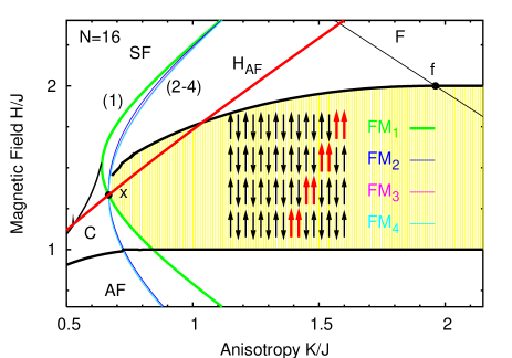
Figure 9: (Color online) High-anisotropy phase diagram for Mills model and $N$=16. The degenerate ferrimagnetic phases are stable in the shaded area. The collinear phases FM₁ and FM₂ to FM₄ are limited by the lability lines (1) and (2-4). The latter are nearly degenerate and not resolved.

As a caveat, we finally have to mention additional low-symmetry phases which cannot be foreseen from the considerations on the stable collinear phases AF, FM_l, and F and their elastic distortions in the phase diagram. Such an intermediate phase C_x appears already in the phase diagram of Mills model for $N=6$ in the region between the FM_l phases and the region of the stable SF-phase. The C_x phase can be derived from an elastic distortion of the collinear phases $\uparrow\downarrow\uparrow\uparrow\uparrow\uparrow$, which do not arise as stable states. Similar low-symmetry canted phases also appear in phase diagrams of Mills model for $N>6$. For generalized models, the region of stability of these canted low-symmetry phases will strongly depend on details of the materials parameters of type Eq. (II.1). Further energy terms and/or disorder in magnetic parameters of the layers can stabilize further phases in the intermediate region of the phase diagram. In the high-anisotropy limit of such generalized models, cascades of metamagnetic transitions between ferrimagnetic collinear phases exist. From these states various canted phases can be derived in the range of intermediate anisotropies $K_{i}/J_{i}\stackrel{{\scriptstyle<}}{{\sim}}1$. The competition between all these phases will lead to very complicated magnetic phase diagram

IV Reorientation in weakly anisotropic multilayers

IV.1 Surface and volume interactions

In this section, we re-analyze the magnetic states of an antiferromagnetic multilayer stack, and their evolution in an applied field, by analytical methods. In the limit of weak anisotropy, the micromagnetic energy (1) can be represented by a system of interacting dimers and by a continuum form. Thus, we consider the model (1) for weak anisotropies, $K_{i},\,K^{\prime}_{i}\ll J_{i}$. Further, we only study systems with collinear antiferromagnetic (zero-field) ground state. Thus, the strengths of the biquadratic exchange constants is limited to the range, $0<\widetilde{J}_{i}<J_{i}/2$.Demokritov98 First, we rewrite the general energy Eq. (1) in this limit. The resulting expression allows to recognize the main effects expected in this limit without explicit calculations. We group the moments of the superlattice into pairs as in a two-sublattice antiferromagnetic system. Starting from the first layer we combine the $N$ moments along the antiferromagnetic chain into $N/2$ pairs $(\mathbf{s}_{2j-1},\mathbf{s}_{2j})$ with $j=1,..,N/2$. For each of these pairs, we introduce the vectors of net magnetization ${\mathbf{M}}_{j}$ and the staggered vector $\mathbf{L}_{j}$

$$\mathbf{s}_{2j-1}={\mathbf{M}}_{j}+\mathbf{L}_{j},\quad\mathbf{s}_{2j}={\mathbf{M}}_{j}-\mathbf{L}_{j}\,.$$ (19)

These transformations are similar to those applied for the two-layer system, Eqs. (5) and (7). From $|\mathbf{s}_{i}|=1$ follows that ${M}_{j}^{2}+L^{2}_{j}=1$ and ${\mathbf{M}}_{j}\cdot\mathbf{L}_{j}=0$. The energy $\Theta_{N}$ of Eq. (1) can be rewritten as a function of ${M}_{j}$ and the angles $\phi_{j}$ between $\mathbf{n}$ and unity vectors $\mathbf{l}_{j}=\mathbf{L}_{j}/|\mathbf{L}_{j}|$ and expanded with respect to the small parameters ${M}_{j}\ll 1$. Omitting constant and higher order terms, one derives

$$\widetilde{\Theta}_{N} = \sum_{j=1}^{N/2}\Lambda_{j}{M}_{j}^{2}-2\sum_{j=1}^{N/2}\left(\mathbf{H}\cdot{\mathbf{M}}_{j}\right)-\sum_{j=1}^{N/2}\widetilde{K}_{i}\cos^{2}\phi_{j}$$ (20)

$$+\frac{1}{2}\sum_{j=1}^{N/2-1}J_{2j}(\phi_{j+1}-\phi_{j})^{2}+\Xi({M}_{j},\phi_{j})\,,$$

where $\widetilde{K}_{j}=(K_{2j-1}+K_{2j})/2-K^{\prime}_{2j-1}-(K^{\prime}_{2j-2}+K^{\prime}_{2j})/2$, $\Lambda_{j}=2(J_{2j-1}-2\widetilde{J}_{2j-1})+(J_{2j-2}-2\widetilde{J}_{2j-2})+(J_{2j}-2\widetilde{J}_{2j})$ for $j=2,\dots,N/2-1$, and $\widetilde{K}_{1}=(K_{1}+K_{2})/2-K^{\prime}_{1}-K^{\prime}_{2}/2$, $\widetilde{K}_{N/2}=(K_{N-1}+K_{N})/2-K^{\prime}_{N-1}-K^{\prime}_{N-2}/2$; $\Lambda_{1}=2(J_{1}-2\widetilde{J}_{1})+(J_{2}-2\widetilde{J}_{2})$, $\Lambda_{N/2}=2(J_{N-1}-2\widetilde{J}_{N-1})+(J_{N-2}-2\widetilde{J}_{N-2})$. Finally, the last expression in Eq. (20) collects terms that are linear with respect to $(\phi_{j+1}-\phi_{j})$,

$$\Xi({M}_{j},\phi_{j}) =$$

$$- \sum_{j=1}^{N/2-1}(J_{2j}-\widetilde{J}_{2j})({M}_{j}+{M}_{j+1})(\phi_{j+1}-\phi_{j})\,.$$

An independent minimization with respect to ${\mathbf{M}}_{j}$ (see details in Ref. [FNT86, ; PRB02, ]) yields

$${\mathbf{M}}_{j}=\Lambda_{j}^{-1}\left[\mathbf{H}-\left(\mathbf{H}\cdot\mathbf{l}_{j}\right)\mathbf{l}_{j}\right]\,.$$ (22)

It follows directly from (22) that ${M}_{j}=H\Lambda_{j}^{-1}\sin(\phi_{j}-\psi)$, where $\psi$ is the angle between the field $\mathbf{H}$ and the easy axis $\mathbf{n}$ in the model of Eq. (1).

The independent minimization with respect to ${\mathbf{M}}_{j}$ is justified because the exchange interactions dominate the energy and pairs of neighbouring moments do not deviate strongly from antiparallel orientation in the limit of weak anisotropy and fields. This establishes the relations Eq. (22) between the components of the net magnetization and the orientation of the staggered vector. In other words Eq. (22) fixedly connects the net magnetizations, as auxiliary degrees of freedom, to the vectors $\mathbf{l}_{j}$ and the applied field. This approach reduces the chain of $N$ magnetic moments $\mathbf{s}_{i}$ into an equivalent system of $N/2$ unity vectors $\mathbf{l}_{j}$. Each site of this chain corresponds to a two-sublattice antiferromagnet or a dimer. Substituting (22) into Eq. (20) we obtain the following expression for the energy of these interacting dimers

$$\widetilde{\Theta}_{N} = -\sum_{j=1}^{N/2}\bar{\Phi}_{j}\cos 2(\phi_{j}-\bar{\phi}_{j})$$

$$+\frac{1}{2}\sum_{j=1}^{N/2-1}J_{2j}(\phi_{j+1}-\phi_{j})^{2}+\Xi(\phi_{j})\,,$$

$$\bar{\Phi}_{j}=\frac{1}{2\Lambda_{j}}\sqrt{\left(H^{2}\cos 2\psi-H_{j}^{2}\right)^{2}+H^{4}\sin^{2}2\psi\;}\,,$$ (24)

$$\tan 2\bar{\phi}_{j} = H^{2}\sin 2\psi/(H^{2}\cos 2\psi-H_{j}^{2}),$$ (25)

$$H_{j} = \sqrt{\widetilde{K}_{j}\Lambda_{j}}\,,$$ (26)

where

$$\Xi(\phi_{j}) = -H\sum_{j=1}^{N/2-1}\Omega_{j}\sin(\phi_{j}-\psi)(\phi_{j+1}-\phi_{j}),$$ (27)

$$\Omega_{j} = J_{2j}\left(\Lambda_{j}^{-1}+\Lambda_{j+1}^{-1}\right)\,.$$ (28)

The minimization with respect to ${\mathbf{M}}_{j}$ according to Eq. (22) and the representation of the energy by the form (IV.1) generalizes simplified dimerization transformation that have been considered in Refs. [pss04, ; JAC, ].

The energy of the interacting dimers Eq. (IV.1) includes first the sum of their “self”-energies, then an exchange stiffness energy given by the term quadratic with respect to differences $(\phi_{j+1}-\phi_{j})$, and a specific energy contribution $\Xi(\phi_{j})$, defined in Eq. (27). The terms in $\Xi(\phi_{j})$ arise due to the variation of the magnetic parameters along the chain. The energy $\Xi(\phi_{j})$ can be written in the form of a “Zeeman energy” for the staggered magnetization vectors

$$\Xi(\phi_{j}) = -\left[\Omega_{1}(\mathbf{H}\cdot\mathbf{l}_{1})-\Omega_{N/2-1}(\mathbf{H}\cdot\mathbf{l}_{N/2})\right]$$

$$-\sum_{j=1}^{N/2-2}\left(\Omega_{j+1}-\Omega_{j}\right)\left(\mathbf{H}\cdot\mathbf{l}_{j+1}\right)\,.$$

The dimensionless coefficients $\Omega_{j}$ are ratios of exchange constants defined in Eq. (28). The first two terms in Eq. (IV.1) involve the endmost dimers, i.e., they have the character of a surface energy, which is imposed by the exchange cut. The sum in (IV.1) describes similar “internal” contributions arising due to any variation of the exchange couplings along the antiferromagnetic chain. This energy contribution disappears in models with equal exchange interactions in internal layers as in the regular and modified Mills models Eqs. II.1) and (II.1), respectively.

IV.2 Physical mechanism of the “surface spin-flop” phenomena

The magnetic energy of the low-anisotropy antiferromagnetic multilayers in the form of interacting dimers (IV.1) elucidates the competing forces responsible for the field-driven reorientation processes. Let us compare energy (IV.1) with that of an isolated dimer. For a localized pair of $\mathbf{s}_{2j-1}$ and $\mathbf{s}_{2j}$ spins (i.e. $j$-th dimer) a minimization via Eq. (22) yields

$$\Theta_{2}^{(j)}=-\Phi_{j}^{(0)}\cos 2(\phi_{j}-\bar{\phi}_{j}^{(0)})\,,$$ (30)

with an amplitude factor

$$\Phi_{j}^{(0)}=\frac{1}{4J}\sqrt{\left(H^{2}\cos 2\psi-\bar{H}_{j}^{2}\right)^{2}+H^{4}\sin^{2}2\psi\;}\,,$$ (31)

and a “phase”

$$\tan 2\bar{\phi}_{j}^{(0)}=H^{2}\sin 2\psi/(H^{2}\cos 2\psi-\bar{H}_{j}^{2}),$$ (32)

where $\bar{H}_{j}^{2}=[(J_{2j-1}-2\widetilde{J}_{2j-1})(K_{2j-1}+K_{2j}+2K^{\prime}_{2j-1})]^{1/2}$. The energy in the form (30) coincides with that of a two-sublattice antiferromagnet and is a generalization of the model Eq. (7). The Eq. (32) for the phase $\bar{\phi}_{j}^{(0)}$ is known as Néel equation.Neel36 It determines the equilibrium states of the antiferromagnet $\phi=\bar{\phi}_{j}^{(0)}+\pi k$ ($k=0,1,\dots$). The amplitude $\Phi_{j}^{(0)}$ from Eq. (31) equals the potential barrier between the wells at $\phi=\bar{\phi}_{1}+\pi k$. A magnetic field applied along the easy axis reduces the potential barrier. When the field reaches the threshold field $\bar{H}_{j}$ it causes the spin-flop transition. For dimers incorporated into the interacting chain the parameters of the self-energies are modified due to the exchange coupling and additional anisotropy contributions as seen by comparing Eqs. (IV.1)-(25) with Eqs. (30)-(32). Therefore, within the chain the dimers have different threshold fields and they are elastically coupled with neighbouring pairs. Due to the couplings the flopping of the individual dimers in their individual threshold fields $H_{j}$ Eq. (IV.1) are hampered. Instead the chain only can transform into the flopped phase when the flopped configurations are energetically advantageous throughout the whole system. Generally the differences of the dimer self-energies along the chain causes spatial modulations of any noncollinear magnetic states. The inhomogeneous spin-flop and canted phases in Mills model (Fig. 3) exemplify such spin-configurations.

However, the energy contribution $\Xi(\phi_{j})$ Eq. (IV.1) provides another mechanism of magnetic-field-induced reorientation imposed by the variation of the exchange interactions along the antiferromagnetic superlattice, in particular by the exchange cut at its ends. This mechanism is due to the influence of the linear energy terms (27), which favour a rotation of the staggered vector. As can be seen from the equivalent Eq. (IV.1), an instability of the collinear configuration is caused by the “Zeeman terms” that are linear in the staggered vectors $\mathbf{l}_{j}$. Generally, the first term related to the two surfaces will dominate, and this difference will favour a rotation of these $\mathbf{l}_{j}$. This enforces an inhomogeneous spin-flop phase above a certain field. As was shown in the previous section in strong anisotropy systems the exchange cut leads to flips of the magnetization and a transition into collinear FM phases, which are also inhomogeneous. In low-anisotropy systems, under the dominating influence of the exchange interactions, the influence of this “local” defect is spread along the chain and stabilizes a spatially inhomogeneous structure.

Thus, we have the following important conclusion. There are two different mechanisms of the field-induced reorientation in finite antiferromagnetic superlattices: (i) One of them is connected with a switching of the potential wells in the energy of the uniaxial antiferromagnetic units. This mechanims is similar to the usual field-driven spin reorientation in (low-anisotropy) bulk antiferromagnets and two-layer systems. Therefore, it is a common spin-flop mechanism. (ii) The other mechanism is due to variation of the exchange coupling along the superlattice and, in particular, the exchange cut at the end of the stack. This type of reorientation transition can only exist in finite antiferromagnetic superlattices and has no analogue in bulk antiferromagnetism.

The interplay of these two mechanisms rules the formation and evolution of the magnetic states in the system. Depending on the values of the material parameters different types of magnetization processes can be realized in the general model (1). In the low-anisotropy systems, owing to the dominance of exchange interactions, it is the second effect due to the cut exchange at the surfaces that dominates the field-driven reorientation transition.

As important cases for applications, we consider in more detail the highly symmetric Mills models Eqs. (II.1) and (II.1). Both models are composed of identical internal layers. For the modified Mills model Eq. (II.1) $\Lambda_{1}=\Lambda_{N/2}=2(2J_{s}+J)/(1+\zeta_{s})$, and $\Lambda_{j}=4J$ for $j=2,\dots,N/2-1$. For the regular Mills model Eq. (II.1) $\Lambda_{j}=4J$ for $j=1,\dots,N/2$. The energy (IV.1) with $\psi=0$ reduces to

$$\tau_{N} = \sum_{j=2}^{N/2-1}\frac{\left(H^{2}-H_{\mathrm{B}}^{2}\right)}{8J}\cos 2\phi_{j}$$

$$+\frac{J}{2}\sum_{j=1}^{N/2-1}(\phi_{j+1}-\phi_{j})^{2}+\Phi_{s},$$

where $H_{\mathrm{B}}=\sqrt{4JK}$. The last contribution in (IV.2) is due to the finite length of the chain. It involves only the two last dimers at both ends of the chain, i.e., it represents the specific surface effects for the finite antiferromagnetic stack. For the regular Mills model the isolated dimer energy (30) reduces to the form of Eq. (9), and the surface energy becomes

$$\Phi_{s} = \frac{1}{6J}\left(H^{2}-H_{S}^{2}\right)\left(\cos 2\phi_{1}+\cos 2\phi_{N/2}\right)$$ (34)

$$-\frac{7}{12}H\left(\cos\phi_{1}-\cos\phi_{N/2}\right)$$

$$+\frac{1}{12}H\left(\cos\phi_{2}-\cos\phi_{N/2-1}\right)\,,$$

$$H_{S} = \sqrt{3JK}\,.$$ (35)

In the case of the modified Mills model, the contribution $\Phi_{s}$ has the modified form

$$\widetilde{\Phi}_{s} = \frac{(1+\zeta_{s})^{2}}{8(2J_{s}+J)}\left(H^{2}-\widetilde{H}_{S}^{2}\right)\left(\cos 2\phi_{1}+\cos 2\phi_{N/2}\right)$$ (36)

$$-U_{1}H\left(\cos\phi_{1}-\cos\phi_{N/2}\right)$$

$$+U_{2}H\left(\cos\phi_{2}-\cos\phi_{N/2-1}\right)\,.$$

The threshold field $\widetilde{H}_{S}$ and the coefficients, $U_{1}$ and $U_{2}$, are defined by

$$\widetilde{H}_{S} = \frac{\sqrt{2(K_{s}+K)(2J_{s}+J)}}{(1+\zeta_{s})},$$ (37)

$$U_{1} = \frac{J(6\zeta_{s}-1)+2J_{s}(4\zeta_{s}-3)}{4(2J_{s}+J)},$$ (38)

$$U_{2} = \frac{J(2\zeta_{s}+1)-2J_{s}}{4(2J_{s}+J)}\,.$$ (39)

The threshold field for the endmost dimers is $H_{S}=\sqrt{3/2}H_{0}$ and for internal dimers $H_{\mathrm{B}}=\sqrt{2}H_{0}$. Because the spins in the chains have additional exchange couplings, these thresholds are larger than the threshold field $H_{0}$ for an isolated pair. This reinforcing by exchange stiffness for the bound dimers increases the values of the threshold fields for the coupled chain.

IV.3 Multilayers with large N. Continuum model

The limit of multilayers with large $N$ and the limit of infinite antiferromagnetic systems is best discussed going over to a continuum description. For the regular Mills model (II.1) with arbitrary $N$ the transition into the flopped state occurs closely to $H_{\mathrm{tr}}\approx H_{0}$ given by Eq. (9), sufficiently below the dimer threshold fields $H_{S}$ and $H_{\mathrm{B}}$ (Fig. 11). This means that this transition is imposed by the exchange cut. These results can be easily understood from the solutions for the spin-configurations in the flopped state Eqs. (10), (11), and (III.1). The magnetization vectors for all internal layers can be combined into pairs with antiparallel magnetizations. The system effectively behaves as an isolated dimer consisting only of the endmost spins with energy (II.1). Correspondingly the flopping field equals the threshold field $H_{0}$ of this isolated pair. This result is common for systems with arbitrary values of $N$.

However, above the critical field $H_{0}$ the evolution of the system remarkably changes with increasing $N$ (Fig. 10). The multilayer with low $N$ are characterized by a large magnetization jump at the transition field and a nearly linear increase of the magnetization up to the flip field. With increasing $N$ the magnetization jump at $H_{0}$ gradually decreases. Concurrently, a steep section of the magnetization curve is found around fields with values close to $H_{\mathrm{B}}$ (see Eq. (IV.2)). Finally, for $N\gg 1$ the magnetization curves develop a strong kink around this value.

The magnetic-field driven transformation of the dimer energies in Eq. (IV.2) explains this peculiar behaviour. In the transition field $H_{\mathrm{tr}}\approx H_{0}$ the dimer self-energy terms in (IV.2) still favour the antiferromagnetic mode $(\mathbf{l}_{j}||\mathbf{n})$. The threshold fields are exceeded at higher fields ($H>H_{S}$ for endmost and $H>H_{\mathrm{B}}$ for internal dimers). In superlattices with few layers the endmost and internal dimers give comparable contributions to the magnetic energy. The difference in their internal energies suppresses drastic reorientation effects at the threshold fields $H_{S}$ and $H_{\mathrm{B}}$. With increasing number of layers the relative energy contribution of the internal dimers for the total energy (20) gradually increases. Then, the magnetic energy of the internal layers plays the dominant role in the formation of the flopped configurations. Thus, the endmost dimers does not hamper the reorientation effects in the threshold field $H_{\mathrm{B}}$. Below the threshold field, $H<H_{\mathrm{B}}$, the antiferromagnetic phase with $\mathbf{l}||\mathbf{n}$ corresponds to the minima of the internal dimers and the inhomogeneous spin-flop phase consists of two antiferromagnetic domains with antiparallel orientation of the staggered vectors (Fig. 11). These two regions are separated by a 180-degree domain wall with flopped spin configurations in the center $(\mathbf{l}\bot\mathbf{n})$

For $H>H_{\mathrm{B}}$ the potential wells for the internal dimers switch into $(\mathbf{l}\bot\mathbf{n})$ configuration. Around the field $H_{\mathrm{B}}$ the center of the domain wall gradually extends and sweeps out the regions with antiferromagnetic configuration towards the surfaces of the stack. This drastic transformation between the two configurations within most of the bulk of the antiferromagnetic stack causes a prominent anomaly of the magnetization curves near the field $H_{\mathrm{B}}$ (Fig. 10). Above $H_{\mathrm{B}}$ the net magnetization $M_{j}$ develops two symmetric maxima close to the surfaces, which may be observable in experiment.

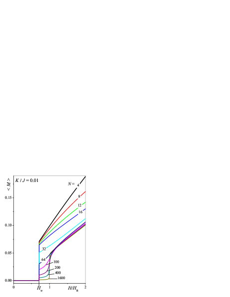
Figure 10: (Color online) Magnetization curves for Mills model with low anisotropy $K/J$=0.01 and large N in the vicinity of the “bulk spin-flop”.

Asymptotically with $N\rightarrow\infty$, the magnetization curve approaches that of the usual spin-flop in a bulk uniaxial antiferromagnet. But, this reorientation occurs within the same magnetic phase, and no phase transition is connected with this process. Rather for any finite value of $N$ the phase transition still occurs between the antiferromagnetic and inhomogeneous spin-flop phase in the critical field $H_{\mathrm{tr}}$ as a first-order process. As was mentioned above for large $N$ this field-induced phase has the character of a domain wall between two antiferromagnetic states. Non-collinear states arise in the central region of the stack, where the small total magnetization of the configuration is concentrated. For fixed small anisotropy the transition is accompanied by a jump of the magnetization at the transition field $H_{\mathrm{tr}}$. The magnitude of this jump decreases with the numbers of layers $N$ (Fig. 10). Hence, at first glance we have a paradox phase diagram for Mills model: a drastic field-driven change of the magnetization is not related to a phase transition, while a real phase transition is noticeable only by a small jump of the magnetization, that vanishes for large $N$. However, this has a clear physical foundation because the transition at $H_{tr}$ is related to the surface effect and its visible effects should vanish for $N\rightarrow\infty$, whereas the crossing-over towards the flopped configuration in the “bulk” of the multilayer stack should approach a true spin-flop transition for $N=\infty$.

A transition into the inhomogeneous spin-flop state means that the free boundaries cause an inhomogeneity far in the interior of the finite system. Close to the boundaries the magnetic configuration resembles that of the two antiferromagnetic collinear domains. This structure is consistent with the properties of semi-infinite antiferromagnetic chains described by Micheletti et al. Micheletti97 In the phase diagrams for these systems (even in the large anisotropy limit) a highly degenerate phase occurs, where a localized inhomogeneous configuration is situated at arbitrary distance from the surface.Micheletti97 For finite antiferromagnetic chains with weak anisotropy, the mutual influence of both surfaces will determine a unique state with 180 degree wall-like configuration in the center. Generally, such a symmetric configuration will be found for antiferromagnetic layers, when the core of this configuration is wide enough to interact with both surfaces. For the finite systems, the simple structure of the phase diagram, showing only a SF phase with solutions preserving mirror symmetry about the center of the layer in intermediate fields between the AF phase and the saturated F phase, is restricted to low anisotropy systems. At sizeable anisotropy, the asymmetric canting complicates the phase-diagram.

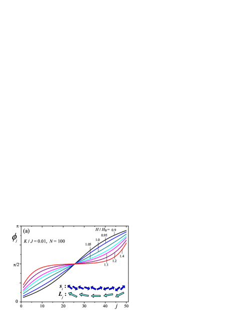
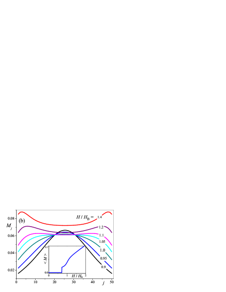
Figure 11: (Color online) Evolution of configurations for Mills model with low anisotropy $K/J$=0.01 and $N=100$ in the vicinity of the “bulk spin-flop”: (a) local net magnetic moments $M_{j}$ (b) orientation of local antiferromagnetic vectors (according to the Eq. (19). Inset shows average magnetization $m$ vs. field.

The energy of the modified Mills model Eq. (II.1) provides a simple way to introduce a continuum form of energy (IV.2). For $N\gg 1$ and low anisotropy $K\ll 1$ the energy (20) can be converted to

$$\Delta W = W-W_{\mathrm{AF}}=$$ (40)

$$\int_{-d/2}^{d/2}\left[A\left(\frac{d\phi}{d\xi}\right)^{2}+\left(\frac{H^{2}-H_{\mathrm{B}}^{2}}{16A}\right)\sin^{2}\phi\right]d\xi$$

$$+W_{s}|_{\xi=\pm d/2}\,$$

with the exchange constant $A=Ja/2$. The multilayer thickness is $d=Na$ with $a$ the “periodicity” length of the multilayer. The zero of energy scale for $\Delta W$ is shifted to the energy $W_{\mathrm{AF}}$ of the antiferromagnetic state ($\phi=0$). The last term is the surface energy given by

$$W_{s} = \frac{(1+\zeta_{s})^{2}}{4(2J_{s}+J)}\left(H^{2}-\widetilde{H}_{S}^{2}\right)\sin^{2}\phi(\xi)$$ (41)

$$- \mathrm{sgn}(\xi)\,\left(\zeta_{s}-\frac{1}{2}\right)H\left[\,\cos\phi(\xi)-1\,\right]$$

Eq. (40) describes the energy of a plate of thickness $d$ for a bulk easy-axis antiferromagnet with the spin-flop field $H_{\mathrm{B}}$. It is the continuum counterpart of the discretized model Eq. (IV.2). The surface energy $W_{s}$ (41) includes a common antiferromagnetic contribution (the first term) and a specific Zeeman energy imposed by the exchange cut. Due to mirror symmetry of the inhomogeneous spin-flop phase the boundary conditions are $\phi_{1}\equiv\phi(\xi=-d/2)$ and $\phi_{2}\equiv\phi(\xi=d/2)=\pi-\phi_{1}$. By solving the Euler equation for the energy functional (40) with the boundary condition $2A(d\phi/d\xi)|_{\xi=\pm d/2}=-\partial W_{s}(\phi 1)/\partial\phi$ one obtains a set of parametrized profiles $\phi(\xi,\phi_{1})$. The further optimization of the energy with respect to the parameter $\phi_{1}$ yields the equilibrium distribution of the staggered vector within the multilayer of finite thickness. These solutions can generally be written as elliptic functions.

In the limit of infinite thickness, $N\rightarrow\infty$ the boundary values of $\phi$ correspond to the configurations in antiparallel domains of the antiferromagnetic phase, $\phi_{1}(-\infty)$ =0, $\phi_{2}(\infty)=\pi$. In this case the variational problem for the functional (40) is equivalent to that of an isolated magnetic wall with “effective uniaxial anisotropy” $K^{*}=(H^{2}-2H_{0}^{2})/(16A)$. The corresponding analytical results for the wall parameters have been derived by Landau and Lifshitz Landau35 . For Mills model this solution has been analysed in Mills68 .

This limiting case of the infinite chain provides a simple physical explanation of the phase transition into the inhomogeneous spin-flop phase. According to Eqs. (40), (41) the flop of the surface staggered vector $\phi(\infty)=0$ into antiparallel position $\phi(\infty)=\pi$ yields a gain of surface energy $\Delta W_{s}=-(2\zeta_{s}-1)H$. By this process a domain wall is generated which requires a positive energy contribution $4\sqrt{AK^{*}}=\sqrt{H_{\mathrm{B}}^{2}-H^{2}\,}$. The balance between these competing energy contributions is reached at the critical field

$$H_{\mathrm{tr}}=H_{0}/\sqrt{2\zeta_{s}^{2}-2\zeta_{s}+1\,}\,.$$ (42)

In particular, for the regular Mills model $\zeta_{s}=1$ and the transition field in Eq. (42) equals $H_{0}$. This simple energetics allows to formulate a clear thermodynamic reason for the transition into the inhomogeneous spin-flop phase provided by the exchange cut. The anti-aligned magnetization vector at the non-compensated surface is overturned and reduces the Zeeman energy at the expense of the formation of a planar defect in the center of the superlattice, which has the character of a domain wall.

Because the energy gain in the inhomogeneous spin-flop phase, $\Delta W_{s}(\zeta_{s})=-(2\zeta_{s}-1)H$, is proportional to the non-compensated magnetization of the surface layer, this transition into the flopped state strongly depends on the net magnetization of the endmost layers. Partial compensation of the surface magnetization is tantamount to a reduction of the parameter $\zeta_{s}$. This reduction decreases $\Delta W_{s}(\zeta_{s})$, and increases the critical field $H_{\mathrm{tr}}$ (42). For $\zeta_{s}=1/2$ the energy gain $\Delta W_{s}(\zeta_{s})$ equals zero and $H_{\mathrm{tr}}$ reaches the threshold field $H_{\mathrm{B}}$.

We come to an important conclusion. The exchange cut provides the stabilization of the flopped phase only under condition of sufficiently strong surface magnetization. In the regular Mills model the magnetizations of the layers are assumed to have fixed values. The properties of the endmost layers $j=1$ and $N$ are described by the same integral phenomenological parameters as the layers $j=2,\dots,N-1$ in the “bulk”. Only the exchange cut reflects the confinement of this antiferromagnetic system. In the continuum limit (40) the surface cut is represented by the surface contributions in the energy that describe the effective coupling of the staggered vector to the applied field. The existence of surfaces with net non-compensated magnetization is justified for antiferromagnetic superlattices with in-plane magnetization. Strong intra-layer exchange interactions and weak stray field effects favour single domain states of the individual ferromagnetic layers in these multilayer stack and at the surfaces. In other systems, various mechanisms can cause reductions of the non-compensated magnetization at the surfaces, such as crystallographic and magnetic imperfections, formation of antiferromagnetic multidomain states etc. A reduction of the total magnetization in the surface layers can strongly reduce the non-compensated magnetization and suppresses eventually the formation of the flopped states. For the continuum model (40) this occurs for $\zeta_{s}<1/2$.

The surface energy (41) also includes the first term that has the conventional form of a (local) antiferromagnetic unit with a modified threshold field $\widetilde{H}_{S}$ from Eq. (37). According to many experimental observations, the magnetic parameters $J_{s}$, $K_{s}$ and $\zeta_{s}$ can be strongly modified by surface-induced interactions, see, e.g., Refs. [Stiles99, ; Johnson96, ]. Correspondingly $\widetilde{H}_{S}$ in (41) can vary in a broad range. Generally, considering models with modified magnetic surface properties, the volume energy (40) and the surface energy (41) may favour different magnetic configurations in certain intervals of applied magnetic field. This competition can stabilize inhomogeneous phases with continuous rotation of the magnetization vectors along the thickness. The occurrence of such twisted states under pinning (or anchoring) influence of the surfaces is a rather general effect in orientable media. In particular, they are known to occur in various classes of liquid crystals as the so-called Freedericksz effect Freed33 ; deGennes and in ferromagnetic materials.Goto65 ; Nolting00 ; Berkowitz99 Spiraling in exchange spring magnets and exchange bias systems also belongs to this class of phenomena.Berkowitz99 The phenomenological theory of such states in antiferromagnetic nanolayers has been developed in Ref. [PRB03, ]. It was shown that non-collinear twisted phases can arise as solutions for magnetic states under anchoring-effects at the surfaces. In contrast to inhomogeneous spin-flop states stabilized by the exchange cut the twisted phases arise due to pinning or distortive effects of surface-induced interactions on the magnetic states. Future analysis of generalized Mills models should concentrate on the combined effects of these surface interactions.

V Discussion

V.1 Solving the “surface spin-flop” puzzle

The exchange cut is the primary driving force that causes the specific reorientation effects in antiferromagnetically ordered multilayers and stabilizes the unique magnetic states unknown in other classes of magnetic systems. The pioneering studies by Mills and co-workers Mills68 ; Wang94 have introduced the notion of a surface-induced instability in confined antiferromagnets Mills68 and of the novel reorientation effects in antiferromagnetic superlattices Wang94 . Mills formulated the basic idea that, in a confined antiferromagnet, uncompensated surface magnetization causes the instability of the collinear state in the applied magnetic field quite below the common (bulk) spin-flop. This transition from the antiferromagnetic to a “surface spin-flop” state should result in flopping a few layers of spins near the surface, i.e., they would turn by nearly 90 degree.Mills68 This picture was improved and detailed by Keffer and Chow,Keffer73 , and supplemented by results of numerical simulations. Wang94 ; Papan98 ; Rakhmanova98 ; Mills99 It constitutes the recent scenario of a “surface spin-flop”. According to this picture the flopped states are nucleated initially at the surface and in increasing fields this surface state moves into the depth of the sample as an antiferromagnetic domain wall: Keffer73 ; Rakhmanova98 “When the external field exceeds the surface spin-flop field, the surface moment, initially antiparallel to the field, rotates nearly by 180^∘. In effect, a twist is applied to one end of the structure. A domain wall is then set up, in an off center position in the finite structure. [$\dots$] With further increase in field, the wall undergoes a series of discontinuous jumps, as it migrates to the center of the structure. [$\dots$] The domain wall becomes centered in the structure, and then with further increase in field broadens, to open up as a flower to evolve into a bulk spin-flop state. The angle between the spins and the external field is less at and near the surface than in the center of the structure.“ Mills99

The detailed investigations of Mills model (II.1) necessitate a considerable revision of the surface spin-flop scenario expanded in Mills68 ; Wang94 and some other papers Keffer73 ; Rakhmanova98 ; Mills99 . This scenario of the surface spin-flop confuses three different types of the solutions for Mills model (II.1), see the phase diagrams in Figs. 3 and 5. The “flopping of a few layers of spins near the surface” is inspired by solutions for ferrimagnetic and canted phases in systems with sizeable anisotropy. The picture of the domain wall movement into the center of the superlattice “in a sequence of discrete hops” Rakhmanova98 is related to cascades of phase transitions between canted phases in superlattices with moderate anisotropy (Figs. 8). Finally, the flower-like broadening of the centered domain wall poetizes the evolution of the inhomogeneous spin-flop phases in fields higher than $H_{\mathrm{B}}$ (Fig. 10).

Thus, the common scenario of the surface spin-flop combines elements that belong to different solutions for different values of the control parameters ($K/J$, $H/J$, $N$) of the model (II.1). In Ref. PRB04 , it was shown that the equations minimizing energy (II.1), as well as general models (1), do not include solutions for surface-confined (localized) states, which were assumed to occur at a “surface spin-flop” transition”. These models own only well-defined “volume” phases and transitions between them.

The term “surface spin-flop” designates the reorientation into the inhomogeneous spin-flop phase at $H_{\mathrm{tr}}$ (line $a-b$ in Fig. 5). Therefore, it is a double misnomer. This transition does not take place at the surface because it involves the reorientation of all spins along the superlattice, i.e., it has a “volume” character. And it is not a proper spin-flop because it is induced by the exchange cut rather than a switching of the potential wells as in the common spin-flops in bulk antiferromagnets.

V.2 Notes on the experimental observations of surface spin-flop phenomena

The concept of a “surface spin-flop” is commonly applied to analyse experimental results in antiferromagnetic superlattices Wang94 ; Felcher02 ; Lauter02 ; Nagy02 . However, the application of an erroneous concept is dangerous. In particular, quantitative conclusions about magnetic materials parameters from the observed reorientation transitions can lead to wrong results. The lability field of the antiferromagnetic states $H_{\mathrm{AF}}$ plays the prime role in the common “surface spin-flop” scenario. Because the surface spin-flop was believed to arise as a local surface instability of the collinear phase exactly at the critical field $H_{\mathrm{AF}}$, this was considered as a transition field into the surface spin-flop state Mills68 ; Keffer73 . In reality a (volume) first-order transition between the antiferromagnetic and inhomogeneous spin-flop phases occurs at $H_{\mathrm{tr}}$ (e.g., the line $a$-$b$ in Fig. 5), which is lower than $H_{\mathrm{AF}}$ (line a$\lambda$) and larger than another lability field $H_{\mathrm{SF}}$ (line $a$-$\alpha$). The interval $H_{\mathrm{SF}}<H<H_{\mathrm{AF}}$ is a metastability region of these competing phases (Fig. 6). In the low-anisotropy limit the metastablity region is extremely small and these characteristic field are all close to the value $H_{0}$ from Eq. (20). In the limit of large anisotropy the lability field $H_{\mathrm{AF}}$ is much larger than the transition field between AF and FM phases (Fig. 5).

The “bulk” spin-flop field is also considered as important element of the common scenario. Starting at $H_{\mathrm{AF}}$ the expansion of the surface spin-flop phase is completed in fields exactly equal to the value of the spin-flop transition in a “bulk” antiferromagnet having the same values of the magnetic parameters as in model (II.1). For low-anisotropy systems this field equals $H_{\mathrm{B}}$ and is $\sqrt{2}$ times larger than the “surface spin-flop” $H_{0}$. This field corresponds to the threshold field for the internal dimers as given in Eq. (IV.2). In systems with large numbers of layers $N$, a strong reorientation of the flopped states occurs in the vicinity of this field. No phase transition is connected with this process, however, it is marked by a noticeable anomaly of the magnetization curve (Fig. 10). Thus, the magnetization curve anomalies are connected with the transition into the flopped state at $H_{\mathrm{tr}}\approx H_{0}$ and with a smooth reorientation near $H_{\mathrm{B}}$ that does not involve a real transition. The ratio $H_{\mathrm{B}}/H_{\mathrm{tr}}$ is about $\sqrt{2}$. A similar anomaly within the spin-flop state is also observed in systems with rather large anisotropy, where the spin-flop phase is preceded by one or several canted phases. However, a glance at the phase diagram, e.g., Fig. 5 shows that there is no simple quantitative relation between the various reorientation anomalies observable in such multilayer systems with sizeable anisotropy.

Magnetic-field-induced reorientation transitions were investigated in high-quality Fe/Cr(211) antiferromagnetic superlattices Wang94 ; Felcher02 . In Ref. [Wang94, ] magnetization curves for Fe/Cr (211) superlattices with strong uniaxial anisotropy were measured by a SQUID magnetometer and by longitudinal magneto-optic Kerr effect. The magnetization curves for both investigated multilayers with even number of layers Cr(100)/[Fe(40)/Cr(11)]₂₂ and Cr(100)/[Fe(20)/Cr(11)]₂₀ demonstrate close correspondence to theoretical results for Mills model. According to Wang94 the values of the antiferromagnetic coupling between the layers is $JM_{0}^{2}$ = 0.275 erg/cm² and uniaxial anisotropy is $KM_{0}^{2}$ = 0.06 erg/cm², The ratio $K/J$ = 0.22 shows that these multilayers belong to the systems at intermediate anisotropy in the phase diagram that display cascades of canted phases. Indeed, the characteristic anomalies in the field derivatives of the magnetization reveal a series of such reorientation transitions. The asymmetric character of these transitions is demonstrated by Kerr measurements (see Fig. 3 (b) in Ref. [Wang94, ]). A cascade of canted phases has also been observed in another Fe/Cr system Felcher02 . In this paper a Cr(100)/[Fe(14)/Cr(11)]₂₀ system has been investigated with $JM_{0}^{2}$ = 0.405 erg/cm² and $KM_{0}^{2}$ = 0.06 erg/cm². The ratio $K/J$ = 0.15 means that this superlattice also evolves in the applied field via a cascade of canted phases. It should be noted that the first-order transitions between these different magnetic phases allows for phase co-existence in rather wide field ranges (see Refs. PRB04a, ; JMMM04, ]). All these processes may involve multidomain states. In the case of multilayers with effective in-plane anisotropy, the stabilization of domain structures will be subject to imperfections. In particular, interface roughness will lead to magnetic charges or leaking dipolar stray fields. The corresponding domain structures is determined by the defect structure of the multilayer and will have an irregular appearance in general (see, e.g., chap. 5.5.7 in Ref. [Hubert98, ]).

In contrast, multilayers with perpendicular anisotropies constitute a novel class of artificial confined antiferromagnets, where well-defined and regular domain structures such as stripes or bubbles can be found. These are layered systems as antiferromagnetically coupled multilayers [CoPt]/Ru Hellwig03 , or Fe-Au superlattices Zoldz04 . These strongly anisotropic systems correspond to the right side of the phase diagrams in Figs. 3, 5 and are characterized by a number metamagnetic jumps Hellwig03 ; JMMM04 . Due to strong demagnetization fields the magnetization processes in these superlattices are accompanied by a complex evolution of multidomain states Hellwig03 ; Hellwig03b ; JMMM04 ; Hellwig05 . Artificial layered systems of this kind with a controlled variation of distinct magnetic states in vertical direction can be considered as artificial metamagnets JMMM04 .

VI Conclusions

In this work, we have provided a complete solution for the basic micromagnetic model of an antiferromagnetic superlattice with ideal non-compensated surfaces under a field along the easy axis. We have shown how one can systematically enumerate and describe the magnetic phases and their transitions for such structures. The puzzle of the variable appearance of “surface spin-flop” phenomena has been resolved by the re-construction of the phase-diagrams and of the limiting cases for this model. To this end various methods had to be introduced that can be used for generalized models. Analytical tools can be efficiently used for all collinear or highly symmetric phases, and for the case of weak anisotropies. Extensions as given by the models Eqs. (1) –(II.1), that include further magnetic coupling terms, additional anisotropies etc., should be made the subject of further work. In particular, the question of competing surface-couplings and partially compensated surfaces in finite antiferromagnetic stacks should be addressed. In such systems, a competition between a genuine inhomogeneous spin-flop phase and twisted states takes place.

In systems with intermediate anisotropies comparable to the indirect interlayer exchange within antiferromagnetic superlattices, one has to expect very complicated phase-diagrams. Still, such situations can be analysed by the micromagnetic methods developed here. However, it is vital to use clear concepts of magnetic phase transitions and clean definitions that designate the driving forces behind the varieties of field-driven reorientation processes in confined antiferromagnets. We emphasize that the notion of a “surface spin-flop” is erroneous because the relevant magnetic energy terms that drive both the canting instabilities at surfaces and the transition into the inhomogeneous spin-flop phase are not related to a balance between effective anisotropies and Zeeman energy in these finite antiferromagnets. The transitions experienced by the type of finite antiferromagnets with non-compensated surfaces, as investigated here, are always related to the exchange cut. Finally, for the artificial antiferromagnetic systems composed of mesoscale ferromagnetic units, the first-order transitions are of crucial importance. The phase-coexistence between states with finite magnetization will give rise to stable domain structures and hysteretic behaviour in these systems owing to demagnetization effects.

- (1) P. Grünberg, R. Schreiber, Y. Pang, M. B. Brodsky, H. Sowers Phys. Rev. Lett. 64, 2304 (1990).
- (2) M. N. Baibich, J. M. Broto, A. Fert, F. Nguyen Van Dau, F. Petroff, P. Etienne, G. Creuzet, A. Friederich, J. Chazelas, Phys. Rev. Lett. 61, 2472 (1988).
- (3) S. A. Wolf, D.D. Awschalom, R.A. Buhrman, J.M. Daughton, S. von Molnar, M.L. Roukes, A.Y. Chtchelkanova, D.M. Treger, Science 294 1488 (2001).
- (4) E. E. Fullerton, D. T. Margulies, N. Supper, H. Do, M. Schabes, A. Berger, A. Moser, IEEE Trans. Magn. 39 639 (2003).
- (5) R. W. Wang, D. L. Mills, E. E. Fullerton, J. E. Mattson, and S. D. Bader, Phys. Rev. Lett. 72, 920 (1994).
- (6) D. L. Mills, J Magn. Magn. Mater. 198-199, 334 (1999).
- (7) O. Hellwig, T. L. Kirk, J. B. Kortright, A. Berger, E. E. Fullerton, Nature Materials 2, 112 (2003).
- (8) O. Hellwig, A. Berger, E. E. Fullerton, Phys. Rev. Lett. 91, 197203 (2003).
- (9) A. Hubert, R. Schäfer, Magnetic Domains (Springer-Verlag, Berlin, 1998).
- (10) S. G. E. te Velthuis, J. S. Jiang, S. D. Bader, G.P. Felcher, Phys. Rev. Lett. 89, 127203 (2002).
- (11) V. Lauter-Pasyuk, H. J. Lauter, B. P. Toperverg, L. Romashev, and V. Ustinov, Phys. Rev. Lett. 89, 167203 (2002); V. Lauter-Pasyuk, H. J. Lauter, B. Toperverg, L. Romashev, M. Minayev, A. Petrenko, V. Aksenov, and V. Ustinov, J. Magn. Magn. Mater. 258-259, 382 (2003).
- (12) F. Nolting et al. Nature 405, 767 (2000); J. Nogues, L. Morellon, C. Leighton, M. R. Ibarra, I. K. Schuller, Phys. Rev. B. 61, R6455 (2000).
- (13) A. N. Bogdanov, U. K. Rößler, Phys. Rev. B. 68, 012407 (2003).
- (14) D. L. Mills, Phys. Rev. Lett. 20, 18 (1968).
- (15) F. Keffer, H. Chow, Phys. Rev. Lett. 31, 1061 (1973).
- (16) S. P. Vernon, R. W. Sanders, A. R. King, Phys. Rev. B. 17, 1460 (1978).
- (17) B. Lüthi, D. L. Mills, R. E. Camley, Phys. Rev. B. 28, 1475 (1983).
- (18) R. H. Barron, P. Mazur, Phys. Rev. B. 36, 5617 (1987).
- (19) J. G. Lepage, R. E. Camley, Phys. Rev. Lett. 65, 1152 (1990).
- (20) R. W. Wang, D. L. Mills, Phys. Rev. B 50, 3931 (1994).
- (21) E. Stryjewski, N. Giordano Adv. Phys. 26, 487 (1977).
- (22) E. A. Turov, Physical Properties of Magnetically Ordered Crystals, Academic Press, New York and London 1965.
- (23) L. Néel, Annales de Physique 5, 232 (1936).
- (24) I. N. J. Poulis, G. E G. Hardeman, Physica 18, 201 (1952); Physica 20, 7 (1954); C. J. Gorter, Rev. Mod. Phys. 25, 332 (1953).
- (25) A. N. Bogdanov, U. K. Rößler, M. Wolf, K.-H. Müller, Phys. Rev. B. 66, 214410 (2002).
- (26) V. G. Bar’yakhtar, A.N. Bogdanov, D. A. Yablonskii, Usp. Fiz. Nauk. 156, 47 (1988) [Sov. Phys. Usp. 31, 810 (1988)].
- (27) M. A. Howson, B. J. Hickey, J. Xu, D. Greig, P. Rhodes, and N. Wiser, Phys. Rev. B 49, 9560 (1994).
- (28) K. Bröhl, S. Di Nunzio, F. Schreiber, Th. Zeidler, H. Zabel, J. App. Phys. 75, 6184 (1994); K. Bröhl, T. Zeidler, F. Schreiber, A. Schreyer, H. Zabel, J. Magn. Magn. Mater. 130, L1 (1994).
- (29) T. Zeidler, F. Schreiber, H. Zabel, J. Appl. Phys. 79, 4793 (1996).
- (30) J. J. Picconatto, M. J. Pechan, E. E. Fullerton, J. Appl. Phys. 81, 5058 (1997).
- (31) C. Chesman, M. A. Lucena, M. C. de Moura, A. Azevedo, F. M. de Aguiar, S. M. Rezende, Phys. Rev. B. 58, 101 (1998).
- (32) P. Srivastava, F. Wilhelm, A. Ney, M. Farle, H. Wende, N. Haack, G. Ceballos, K. Baberschke, Phys. Rev. B. 58, 5701 (1998); F. May, P. Srivastava, M. Farle, U. Bovensiepen, H. Wende, R. Chauvistre, K. Baberschke, J. Magn. Magn. Mater. 177, 1220 (1998).
- (33) J. Z. Hilt, J. J. Picconatto, A. O’Brien, M. J. Pechan, E. E. Fullerton, J. Magn. Magn. Mater. 199, 387 (1999).
- (34) K. Temst, E. Kunnen, V. V. Moshchalkov, H. Maletta, H. Fritzsche, and Y. Bruynseraede, Physica B 276-278, 684 (2000).
- (35) M. R. Fitzsimmons, P. Yashar, C. Leighton, I. K. Schuller, J. Nogu s C. F. Majkrzak and J. A. Dura, Phys. Rev. Lett. 84, 3986 (2000); C. Leighton, M.R. Fitzsimmons, P. Yashar, A. Hoffmann, J. Nogues, J. Dura, C.F. Majkrzak, I.K. Schuller, Phys. Rev. Lett. 86, 4394 (2001).
- (36) P. Vavassori, M. Grimsditch, E. E. Fullerton J. Magn. Magn. Mater. 223, 284 (2001).
- (37) D. L. Nagy, L. Bottýan, B. Croonenborghs, L. Deák, B. Degroote, J. Dekoster, H.J. Lauter, V. Lauter-Pasyuk, O. Leupold, M. Major, J. Meersschaut, O. Nikonov, A. Petrenko, R. Rüffer, H. Spiering, and E. Szilágyi, Phys. Rev. Lett. 88, 157202 (2002); L. Bottýan, L. Deák, J. Dekoster, E. Kunnen, G. Langouche, J. Meersschaut, M. Major, D. L. Nagy, H. D. Rüter, E. Szilágyi, and K, Temst, J. Magn. Magn. Mater. 240, 514 (2002).
- (38) F. G. Aliev, J. L. Martinez, V. V. Moshchalkov, Y. Braynseraede, A. P. Levanyuk, R. Villar, Phys. Rev. Lett. 88, 187201 (2002).
- (39) H. J. Lauter, V. Lauter-Pasyuk, B.P. Toperverg, U. Rücker, M. Milyaev, L. Romashev, T. Krinitsyna, V. Ustinov, Physica B 335, 59 (2003).
- (40) L. Trallori, P. Politi, A. Rettori, M. G. Pini, J. Villain, Phys. Rev. Lett. 72, 1925 (1994).
- (41) L. Trallori, P. Politi, A. Rettori, M. G. Pini, J. Villain, J. Phys.: Condens. Matter 7, L451 (1995).
- (42) A. S. Carriço, R. E. Camley, R. L. Stamps, Phys. Rev. B 50, 13453 (1994).
- (43) C. Micheletti, R. B. Griffiths, and J.M. Yeomans, J. Phys. A: Math. Gen. 30, L233 (1997); C. Micheletti, R. B. Griffiths, and J.M. Yeomans, Phys. Rev. B 59, 6239 (1999).
- (44) S. G. Chung, J. Phys.: Condens. Matter 13, L219 (1997).
- (45) S. Rakhmanova, D. L. Mills, and E. E. Fullerton, Phys. Rev. B. 57, 476 (1998).
- (46) N. Papanicolaou, J. Phys.: Condens. Matter 10, L131 (1998); N. Papanicolaou, J. Phys.: Condens. Matter 11, 59 (1999).
- (47) M. Momma, T. Horiguchi, Physica A 259, 105 (1998).
- (48) A. S. Zhedanov, A. N. Maluk, Theor. Math. Phys. 115, 584 (1998).
- (49) A. L. Dantas, A. S. Carriço, Phys. Rev. B 59, 1223 (1999).
- (50) J. Karadamoglou, N. Papanicolaou, J. Phys. A: Math. Gen. 32, 3275 (1999); Phys. Rev. B. 60, 9477 (1999).
- (51) X. Wang, X. Zotos, J. Karadamoglou, N. Papanicolaou, Phys. Rev. B. 61, 14303 (2000).
- (52) L. Trallori, Phys. Rev. B. 57, 5923 (1998).
- (53) U. K. Rößler, A. N. Bogdanov, Phys. Rev. B. 69, 094405 (2004).
- (54) U. K. Rößler, A. N. Bogdanov, phys. stat. sol. (c) 1, 3297 (2004).
- (55) U. K. Rößler, A. N. Bogdanov, Phys. Rev. B. 69, 184420 (2004).
- (56) U. K. Rößler, A. N. Bogdanov, J. Magn. Magn. Mater. 269, L287 (2004).
- (57) A. Thiaville and A. Fert, J. Magn. Magn. Mater. 113, 161 (1992).
- (58) A. N. Bogdanov and U. K. Rößler, Phys. Rev. Lett. 87, 037203 (2001); A. N. Bogdanov, U. K. Rößler, and K.-H. Müller, J. Magn. Magn. Mater. 238, 155 (2002).
- (59) V. V. Ustinov, M.A. Milyaev, L.N. Romashev, T.P. Krinitsina, E.A. Kravtsov, J. Magn. Magn. Mater. 226-230, 1811 (2001).
- (60) M.T. Johnson, P. J. H. Bloemen, F. J. A. den Broeder, J. J. de Vries, Rep. Prog. Phys. 59, 1409 (1996).
- (61) M. Rührig, R. Schäfer, A. Hubert, R. Mosler, J.A. Wolf, S. Demokritov, and P. Grünberg, phys. stat. sol. A 125, 635 (1991).
- (62) S. O. Demokritov, J. Phys. D: Appl. Phys. 31, 925 (1998).
- (63) H. Itoh, H. Yanagihara, K. Suzuki, E. Kita, J. Magn. Magn. Mater. 257, 184 (2003).
- (64) O. Hellwig, A. Berger, E. E. Fullerton, J. Magn. Magn. Mater. 290-291, 1 (2005).
- (65) P. Moriarty, Rep. Prog. Phys. 64, 297 (2001); S. D. Bader, Surf. Sc. 500, 172 (2002); NEW review by S. D. Bader, RMP.
- (66) A.N. Bogdanov, Fiz. Nizk. Temp. 12, 515 (1986) [Sov. J. Low Temp. Phys. 12, 290 (1986)].
- (67) U. K. Rößler, A. N. Bogdanov, J. Alloys and Compounds, in press (2006).
- (68) L. D. Landau, E. M. Lifshitz, Phys. Z. Sowietunion 8 135 (1935).
- (69) M. D. Stiles, J. Magn. Magn. Mater. 200, 322(1999).
- (70) V. Freedericksz, V. Zolina, Trans. Faraday Soc. 29, 919 (1933); H. Zocher, Trans. Faraday Soc. 29, 945 (1933).
- (71) P. G. de Gennes, J. Prost, The Physics of Liquid Crystals (Clarendon , Oxford 1993).
- (72) E. Goto, N. Hayashi, T. Miyashita, and K. Nakagawa, J. Appl. Phys. 36, 2951 (1965); A. Thiaville, A. Fert, J. Magn. Magn. Mater. 113, 161 (1992).
- (73) A. E. Berkowitz, K. Takano, J. Magn. Magn. Mater. 200, 552 (1999); J. Nogues, I. K. Schuller, J. Magn. Magn. Mater. 192, 203 (1999).
- (74) M. Zoldz, T. Slezak, D. Wikgocka-Slezak, N. Spiridis, J. Korecki, T. Stobiecki, K. Roll, J. Magn. Magn. Mater. 272, 1253 (2004).