Phase diagram of the anisotropic multichannel Kondo Hamiltonian revisited

Abstract

The phase diagram of the multichannel Kondo Hamiltonian with an XXZ spin-exchange anisotropy is revisited, revealing a far richer fixed-point structure than previously appreciated. For a spin-$\frac{1}{2}$ impurity and $k>2$ conduction-electron channels, a second ferromagnetic-like domain is found deep in the antiferromagnetic regime. The new domain extends above a (typically large) critical longitudinal coupling $J_{z}^{\ast}>0$, and is separated from the antiferromagnetic domain by a second Kosterliz-Thouless line. A similar line of stable ferromagnetic-like fixed points with a residual isospin-$\frac{1}{2}$ local moment is shown to exist for large $J_{z}\gg|J_{\perp}|>0$ and arbitrary $k$ and $s$ obeying $|k-2s|>1$. Here $J_{z}$ is the longitudinal spin-exchange coupling, $J_{\perp}$ is the transverse coupling, and $s$ is the impurity spin. Near the free-impurity fixed-point, spin-exchange anisotropy is a relevant perturbation for $s>1/2$ and arbitrary $k$. Depending on the sign of $J_{z}^{2}-J_{\perp}^{2}$ and the parity of $2s$, the system flows either to a conventional Fermi liquid with no residual degeneracy, or to a $k$-channel, spin-$\frac{1}{2}$ Kondo effect, or to a line of ferromagnetic-like fixed points with a residual isospin-$\frac{1}{2}$ local moment. These results are obtained through a combination of perturbative renormalization-group techniques, Abelian bosonization, a strong-coupling expansion in $1/J_{z}$, and explicit numerical renormalization-group calculations.

I Introduction and overview of results

For over the last forty years, the Kondo effect has occupied a central place in condensed matter physics. While earlier studies of the effect have focused on its single-channel version realized in dilute magnetic alloys and valence-fluctuating systems, later attention has largely shifted to its more exotic multichannel variants where deviations from conventional Fermi-liquid behavior can be found. The overscreened Kondo effect is a paradigmatic example for quantum criticality in quantum-impurity systems. Besides the possible relevance to certain heavy fermion alloys, Cox87 ; Seaman_etal_91 ballistic metal point contacts, RB92 ; RLvDB94 scattering off two-level tunneling systems, Zawadowski80 ; VZ83 ; ThAsSe and the charging of small metallic grains, Matveev91 ; Ashoori99 the overscreened Kondo effect is one of the rare examples of interaction-driven non-Fermi-liquid behavior that is well understood and well characterized theoretically. CZ98 The underscreened Kondo effect, which might be realized in ultrasmall quantum dots with an even number of electrons, PC05 is a prototype for yet another form of unconventional behavior — that of a singular Fermi liquid. Mehta-etal05

These vastly different ground states, as well as that of an ordinary Fermi liquid, can all be described within the single framework of the multichannel Kondo Hamiltonian, which is among the simplest yet richest models for strong electronic correlations in condensed-matter physics. The multichannel Kondo Hamiltonian of Eq. (3) describes the spin-exchange interaction of a spin-$s$ local moment with $k$ identical, independent bands of spin-$\frac{1}{2}$ electrons. For antiferromagnetic exchange, the low-energy physics features a subtle interplay between $k$ and $s$, which could be summarized as follows. CZ98 For $k=2s$, the impurity spin is exactly screened. A spin singlet progressively forms below a characteristic Kondo temperature $T_{K}$, leading to the formation of a local Fermi liquid. For $k>2s$, the impurity spin is overscreened by the $k$ conduction-electron channels. The system flows to an intermediate-coupling, non-Fermi-liquid fixed point, characterized by anomalous thermodynamic and dynamical properties. The elementary excitations are collective in nature, in contrast to the concept of a Fermi liquid. For $k<2s$, the impurity spin is underscreened. The low-energy physics comprises of quasiparticle excitations plus a residual moment of size $s^{\prime}=s-k/2$. However, it differs from a conventional Fermi liquid in the singular energy dependence of the scattering phase shift and divergence of the quasiparticle density of states. Mehta-etal05 ; CP03 ; KHM05 Such behavior was recently termed a singular Fermi liquid. Mehta-etal05 Similar qualitative behavior is found for ferromagnetic exchange with arbitrary $k$ and $s$, except that the residual moment has the full spin $s$.

Inherent to some of the leading scenarios for the realization of the multichannel Kondo model Zawadowski80 ; VZ83 ; Matveev91 is a large spin-exchange anisotropy. An XXZ anisotropy is well known to be irrelevant both in the single-channel ($k=1$, $s=1/2$) and the two-channel ($k=2$, $s=1/2$) cases. The accepted phase diagram for these two models consists of an antiferromagnetic and a ferromagnetic domain, separated by a Kosterliz-Thouless line that traces $J_{z}=-|J_{\perp}|$ at weak coupling. Here $J_{z}$ and $J_{\perp}$ are the longitudinal and transverse exchange couplings, respectively. As long as one lies within the confines of the antiferromagnetic domain, the system flows to the isotropic spin-exchange fixed point regardless of how large the exchange anisotropy is.

Far less explored is the role of spin-exchange anisotropy for either $s>1/2$ or $k>2$. The stability of the overscreened fixed point against weak spin-exchange anisotropy has been analyzed in Ref. ALPC92, using conformal field theory. For $k>1$ and either $s=1/2$ or $s=(k-1)/2$, the non-Fermi-liquid fixed point was found to be stable against a weak spin-exchange anisotropy. This has led to the perception that spin-exchange anisotropy is irrelevant for these values of $k$ and $s$. In contrast, spin-exchange anisotropy is a relevant perturbation at the overscreened fixed point for all other values of $1/2<s<(k-1)/2$ (assuming $k>4$; for $k=4$ it is a marginal perturbation), ALPC92 though the nature of the anisotropic fixed points was never explored. Likewise unexplored is the effect of spin-exchange anisotropy on the underscreened fixed point for $s>k/2$.

In this paper, we revisit the phase diagram of the multichannel Kondo model with an XXZ spin-exchange anisotropy. We find a far more complex picture than previously appreciated, including new coupling regimes where an XXZ anisotropy substantially alters the low-energy physics. Our main findings are as follows.

• For $s=1/2$ and $k>2$, a second ferromagnetic-like domain is found deep in the antiferromagnetic regime. The new domain extends above a (typically large) critical longitudinal coupling $J_{z}^{\ast}>0$, and is separated from the conventional antiferromagnetic (non-Fermi-liquid) domain by a second Kosterliz-Thouless line.

• For spin $s>1/2$ and arbitrary $k$, spin-exchange anisotropy is relevant near the free-impurity fixed point. For sufficiently small $0<|\rho J_{\perp}|<|\rho J_{z}|\ll 1/ks$ ($\rho$ is the conduction-electron density of states per lattice site), the system flows to a line of stable ferromagnetic-like fixed points with a residual isospin-$\frac{1}{2}$ moment. For sufficiently small $|\rho J_{z}|<|\rho J_{\perp}|\ll 1/ks$, the flow is either to a conventional Fermi liquid with no residual degeneracy (for half-integer $s$), or to a $k$-channel Kondo effect with an effective spin-$\frac{1}{2}$ local moment (for integer $s$). Here by sufficiently small $\rho J_{z}$ and $\rho J_{\perp}$ we mean the limit $J_{z},J_{\perp}\to 0$ with any fixed ratio $r=J_{z}/J_{\perp}\neq\pm 1$. The closer $|r|$ is to one, the smaller the couplings must be for these results to apply.

• For $|k-2s|>1$ and a sufficiently large $J_{z}\gg|J_{\perp}|>0$, the system flows to a line of stable ferromagnetic-like fixed points with a residual isospin-$\frac{1}{2}$ moment. Only for $k=2s$ and $k=2s+1$ are the exactly screened and overscreened fixed points stable against such a large anisotropy, which is marginal for $k=2s-1$.

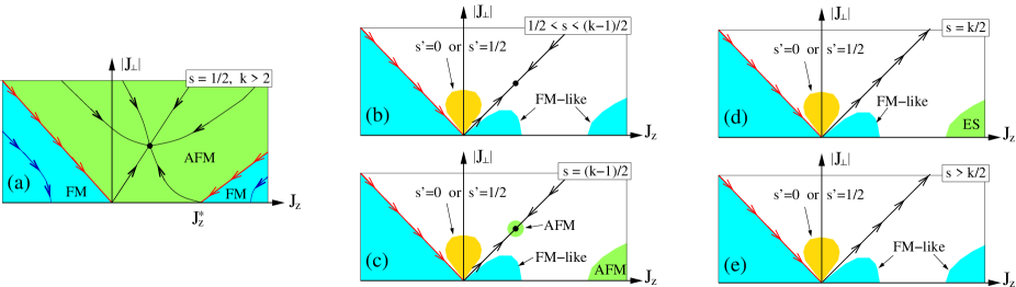
Figure 1: (Color online) Phase diagram of the multichannel Kondo model for the different categories of $s$ and $k$. (a) $s=1/2$ and $k>2$. In addition to the well-established ferromagnetic domain for $J_{z}\leq-|J_{\perp}|$, a second ferromagnetic-like domain extends to the right and below the red line stretching from $(J_{z},J_{\perp})=(J_{z}^{\ast},0)$. Within bosonization, $J_{z}^{\ast}$ is given by Eq. (37). (b) $1/2<s<(k-1)/2$. In addition to the conventional ferromagnetic domain for $J_{z}\leq-|J_{\perp}|$, the system flows to a line of stable ferromagnetic-like fixed points with a residual isospin-$\frac{1}{2}$ local moment in two opposite limits: (i) for sufficiently small $J_{z}>|J_{\perp}|$, (ii) for sufficiently large $J_{z}\gg|J_{\perp}|,D$ ($D$ being the conduction-electron bandwidth). For weak $|J_{\perp}|>|J_{z}|$, the system flows either to a Fermi-liquid fixed point with a frozen impurity (for integer $s$), or to an overscreened $k$-channel, spin-$\frac{1}{2}$ Kondo effect (for half-integer $s$). The above weak-coupling behavior is generic to $s>1/2$. It extends to all cases described below, irrespective of $k$. (c) $s=(k-1)/2$. In contrast to (b), the isotropic overscreened fixed point is stable against a weak spin-exchange anisotropy (i.e., in the vicinity of the overscreened fixed point), as well as against a sufficiently large $J_{z}\gg|J_{\perp}|,D$. (d) $s=k/2$. The exactly screened fixed point, corresponding to strong coupling, is stable against a sufficiently large anisotropy, $J_{z}\gg|J_{\perp}|,D$. However, it is unstable at weak coupling, as described above. (e) $s>k/2$. All underscreened cases flow to a line of stable ferromagnetic-like fixed points with a residual isospin-$\frac{1}{2}$ local moment both for sufficiently large $J_{z}\gg|J_{\perp}|$ and for sufficiently small $J_{z}>|J_{\perp}|$.

A compilation of these results is presented in Fig. 1, in the form of phase diagrams for the different categories of $s$ and $k$. The phase diagrams for $s>1/2$ are still incomplete. There remain extended coupling regimes where the low-energy physics is yet to be determined.

To obtain these results, we employ a combination of perturbative renormalization-group (RG) techniques, Abelian bosonization, a strong-coupling expansion in $1/J_{z}$, and explicit numerical renormalization-group Wilson75 calculations. Using perturbative RG we first analyze in Sec. II the limit of weak coupling. In addition to the standard RG equations for the dimensionless couplings $\rho J_{z}$ and $\rho J_{\perp}$, a new Hamiltonian term proportional to $S_{z}^{2}$ is generated for $s>1/2$ and $J_{z}\neq J_{\perp}$. Here $S_{z}$ is the $z$ component of the impurity spin. Depending on the sign of $J_{z}^{2}-J_{\perp}^{2}$, the new Hamiltonian term favors either the maximally polarized impurity states ($S_{z}=\pm s$) or the minimally polarized ones. This leads to a qualitative distinction between $J_{z}>|J_{\perp}|$ and $|J_{\perp}|>|J_{z}|$, and to the different low-temperature behaviors described above.

Proceeding with Abelian bosonization, we next show in Sec. III that the anisotropic multichannel Kondo Hamiltonian with $s=1/2$ and $k>1$ possesses an exact mapping between the two sets of coupling constants $(J_{z},J_{\perp})$ and $(J^{\prime}_{z},J_{\perp})$, where

$$\arctan\left(\frac{\pi\rho J^{\prime}_{z}}{4}\right)=\frac{\pi}{k}-\arctan\left(\frac{\pi\rho J_{z}}{4}\right).$$ (1)

The above mapping is restricted to values of $J_{z}$ where the right-hand side of Eq. (1) does not exceed $\pi/2$. For $k=2$, this condition limits the validity of the mapping to $J_{z}\geq 0$, in which case Eq. (1) simplifies to

$$\rho J^{\prime}_{z}=\left(\frac{4}{\pi}\right)^{2}\frac{1}{\rho J_{z}}.$$ (2)

For $k>2$, the mapping extends to negative values of $J_{z}$, relating $J_{z}>J_{z}^{\ast}=(4/\pi\rho)\tan(\pi/k)$ to $J_{\rm min}\leq J^{\prime}_{z}<0$ and vice versa [see Eq. (36) for definition of $J_{\rm min}$]. Thus, in contrast to common perception, the multichannel Kondo Hamiltonian with $s=1/2$ and $k>2$ possesses a line of stable ferromagnetic-like fixed points for $J_{z}>J_{z}^{\ast}$. Note, however, that $J_{z}^{\ast}$ exceeds the bandwidth for intermediate values of $k$, and is pushed to weak coupling for $k\gg 1$.

Interestingly, the mapping of Eq. (1) is ingrained in the Anderson-Yuval approach to the multichannel Kondo problem, devised in Refs. FGN95, and Ye96, . In fact, it was already recognized by Fabrizio et al. for $k=2$, FGN95 but was never appreciated to our knowledge for $k>2$. Here we provide an explicit operator mapping between the two sets of model parameters, for arbitrary $k>1$.

Since the critical coupling $J_{z}^{\ast}$ predicted by Eq. (1) is typically larger than the bandwidth, one might question the applicability of bosonization and its unbound linear dispersion. Could it be that $J_{z}^{\ast}\to\infty$ when the conduction electrons are placed on a lattice? To eliminate this concern, a strong-coupling expansion in $1/J_{z}$ is carried out in Secs. IV and V, first for $s=1/2$ and then for arbitrary $s$. The strong-coupling expansion not only confirms the existence of the new line of stable ferromagnetic-like fixed points for $s=1/2$ and $k>2$, but further extends this result to arbitrary $s$ and $k$ obeying $|k-2s|>1$. For $k=2s$ and $k=2s+1$, it establishes the irrelevance of such a large anisotropy.

As an explicit demonstration of these ideas, the phase diagram of the $s=1/2$, $k=3$ model is studied in Sec. VI using Wilson’s numerical renormalization-group (NRG) method. Wilson75 The NRG results confirm the phase diagram inferred from Eq. (1), including the order of magnitude of the critical coupling $J_{z}^{\ast}$. An extension of the mapping of Eq. (1) to a spin-one impurity is presented in turn in Appendix A. We conclude in Sec. VII with a discussion and summary of our results.

II Weak coupling

We begin our discussion with the limit of weak coupling, which is treated using perturbative RG. In the standard notation, the multichannel Kondo Hamiltonian reads

$${\cal H} = \sum_{n=1}^{k}\sum_{\sigma=\uparrow,\downarrow}\sum_{\vec{k}}\epsilon_{\vec{k}}c^{\dagger}_{\vec{k}n\sigma}c_{\vec{k}n\sigma}$$ (3)

$$+ \frac{J_{z}}{2N}\sum_{n=1}^{k}\sum_{\vec{k},\vec{k}^{\prime}}\left[c^{\dagger}_{\vec{k}n\uparrow}c_{\vec{k}^{\prime}n\uparrow}-c^{\dagger}_{\vec{k}n\downarrow}c_{\vec{k}^{\prime}n\downarrow}\right]S_{z}$$

$$+ \frac{J_{\perp}}{2N}\sum_{n=1}^{k}\sum_{\vec{k},\vec{k}^{\prime}}\left[c^{\dagger}_{\vec{k}n\uparrow}c_{\vec{k}^{\prime}n\downarrow}S^{-}+c^{\dagger}_{\vec{k}n\downarrow}c_{\vec{k}^{\prime}n\uparrow}S^{+}\right]\!.$$

Here, $c^{\dagger}_{\vec{k}n\sigma}$ creates an electron with wave number $\vec{k}$ and spin projection $\sigma$ in the $n$th conduction-electron channel; $\vec{S}$ is a spin-$s$ operator; $J_{z}$ and $J_{\perp}$ are the longitudinal and transverse Kondo couplings, respectively; and $N$ is the number of lattice sites.

As a first step toward devising a perturbative RG treatment of the Hamiltonian of Eq. (3), we convert the model to dimensionless form. To this end, we introduce the fermion operators

$$a^{\dagger}_{\varepsilon n\sigma}=\frac{1}{\sqrt{D\rho(E)N}}\sum_{\vec{k}}\delta(\varepsilon-\epsilon_{\vec{k}}/D)c^{\dagger}_{\vec{k}n\sigma},$$ (4)

which represent the $2k$ conduction-electron modes that couple to the impurity within the energy shell $E=\varepsilon D$. Here $D$ is the conduction-electron bandwidth and $\rho(E)$ is the conduction-electron density of states per lattice site:

$$\rho(E)=\frac{1}{N}\sum_{\vec{k}}\delta(E-\epsilon_{\vec{k}}).$$ (5)

The dimensionless operators $a^{\dagger}_{\varepsilon n\sigma}$ have been normalized to obey canonical anticommutation relations:

$$\left\{a_{\varepsilon n\sigma},a^{\dagger}_{\varepsilon^{\prime}n^{\prime}\sigma^{\prime}}\right\}=\delta_{nn^{\prime}}\delta_{\sigma\sigma^{\prime}}\delta(\varepsilon-\varepsilon^{\prime}).$$ (6)

Assuming a box density of states $\rho(E)=\rho\theta(D-|E|)$ and omitting all modes that decouple from the impurity, Eq. (3) is recast in the form ${\cal H}=D\tilde{\cal H}$, where $\tilde{\cal H}$ is the dimensionless Hamiltonian

$$\tilde{\cal H} = \sum_{n=1}^{k}\sum_{\sigma=\uparrow,\downarrow}\int_{-1}^{1}\varepsilon a^{\dagger}_{\varepsilon n\sigma}a_{\varepsilon n\sigma}d\varepsilon$$ (7)

$$+ \frac{\tilde{J}_{z}}{2}\sum_{n=1}^{k}\int_{-1}^{1}\!d\varepsilon\int_{-1}^{1}\!d\varepsilon^{\prime}\left[a^{\dagger}_{\varepsilon n\uparrow}a_{\varepsilon n\uparrow}-a^{\dagger}_{\varepsilon n\downarrow}a_{\varepsilon n\downarrow}\right]S_{z}$$

$$+ \frac{\tilde{J}_{\perp}}{2}\sum_{n=1}^{k}\int_{-1}^{1}\!d\varepsilon\int_{-1}^{1}\!d\varepsilon^{\prime}\left[a^{\dagger}_{\varepsilon n\uparrow}a_{\varepsilon n\downarrow}S^{-}+{\rm H.c.}\right].$$

Here $\tilde{J}_{z}=\rho J_{z}$ and $\tilde{J}_{\perp}=\rho J_{\perp}$ are the dimensionless Kondo couplings.

Focusing on $|\tilde{J}_{z}|,|\tilde{J}_{\perp}|\ll 1/ks$, we treat the Hamiltonian of Eq. (7) using perturbative RG. The RG transformation consists of the following three steps. Suppose that the bandwidth has already been lowered from its initial value $D$ to some value $D^{\prime}=De^{-l}$ ($l>0$). Further lowering the bandwidth to $D^{\prime\prime}=D^{\prime}(1-\delta l)$ requires the elimination of all $a_{\varepsilon n\sigma}$ degrees of freedom in the interval $1-\delta l<|\varepsilon|\leq 1$. This goal is accomplished using Anderson’s poor-man’s scaling. Anderson70 At the conclusion of this step, all integrations in Eq. (7) have been reduced to the range $-(1-\delta l)\leq x\leq 1-\delta l$. The RG transformation is completed by (i) rescaling $\tilde{\cal H}\to\tilde{\cal H}/(1-\delta l)$ to account for the reduced bandwidth, and (ii) restoring the original integration ranges in Eq. (7) by converting to

$$a_{\varepsilon n\sigma}\to\tilde{a}_{\varepsilon n\sigma}=(1-\delta l)^{1/2}a_{(1-\delta l)\varepsilon n\sigma}.$$ (8)

This latter step allows us to write

$$\int_{-(1-\delta l)}^{1-\delta l}a_{\varepsilon n\sigma}d\varepsilon=(1-\delta l)^{1/2}\int_{-1}^{1}\tilde{a}_{\varepsilon n\sigma}d\varepsilon.$$ (9)

The dimensionless Hamiltonian is recast in this manner in a self-similar form, but with renormalized couplings. These obey a set of coupled differential equations, specified below.

For $s=1/2$ we recover the familiar RG equations

$$\frac{d\tilde{J}_{z}}{dl} = \tilde{J}_{\perp}^{2},$$ (10)

$$\frac{d\tilde{J}_{\perp}}{dl} = \tilde{J}_{\perp}\tilde{J}_{z},$$ (11)

showing that spin-exchange anisotropy is irrelevant for weak $\tilde{J}_{z}>-|\tilde{J}_{\perp}|$, irrespective of the number of channels $k$. A different qualitative picture emerges for spin $s$ larger than one-half. Here a new Hamiltonian term $\tilde{\Delta}S_{z}^{2}$ is generated within $\tilde{\cal H}$. Starting from zero, $\tilde{\Delta}$ renormalizes according to

$$\frac{d\tilde{\Delta}}{dl}=\tilde{\Delta}-k\ln(2)\left[\tilde{J}_{z}^{2}-\tilde{J}_{\perp}^{2}\right],$$ (12)

which supplements Eqs. (10) and (11) for $\tilde{J}_{z}$ and $\tilde{J}_{\perp}$. Restricting attention to $s>1/2$, we now analyze the ramifications of the new coupling $\tilde{\Delta}$ as a function of $s$, $k$, and the bare Kondo couplings $J_{z}$ and $J_{\perp}$.

Since $\tilde{J}_{z}^{2}-\tilde{J}_{\perp}^{2}$ is conserved under the RG, a negative (positive) $\tilde{\Delta}$ is generated if the bare Kondo couplings satisfy $|J_{z}|>|J_{\perp}|$ ($|J_{z}|<|J_{\perp}|$). For a given ratio $J_{z}/J_{\perp}\neq\pm 1$ and sufficiently small $|J_{\perp}|$, the coupling $|\tilde{\Delta}|$ approaches unity well before any Kondo temperature can be reached. This has the effect of freezing all but the lowest-lying spin states. For $|J_{z}|>|J_{\perp}|$ (negative $\tilde{\Delta}$), only the maximally polarized states $S_{z}=\pm s$ are thus left. For $|J_{z}|<|J_{\perp}|$ (positive $\tilde{\Delta}$), the picture depends on $s$: for half-integer $s$, the two degenerate states $S_{z}=\pm 1/2$ are selected; for integer $s$, only the state $S_{z}=0$ remains.

Depending on which case is realized, a different effective low-energy Hamiltonian emerges. Consider first the case $|J_{z}|>|J_{\perp}|$ (negative $\tilde{\Delta}$). Introducing the isospin operators

$$\tau_{z}=\frac{1}{2}|s\rangle\langle s|-\frac{1}{2}|-s\rangle\langle-s|,$$ (13)

$$\tau^{\pm}=|\pm s\rangle\langle\mp s|,$$ (14)

the resulting low-energy Hamiltonian contains the term

$$\tilde{\cal H}_{J_{z}}=s\tilde{J}_{z}\sum_{n=1}^{k}\int_{-1}^{1}\!d\varepsilon\int_{-1}^{1}\!d\varepsilon^{\prime}\left[a^{\dagger}_{\varepsilon n\uparrow}a_{\varepsilon n\uparrow}-a^{\dagger}_{\varepsilon n\downarrow}a_{\varepsilon n\downarrow}\right]\tau_{z},$$ (15)

which follows from projection of the spin-exchange interaction of Eq. (7) onto the $S_{z}=\pm s$ subspace. Here ${\tilde{J}}_{z}$ is the running coupling constant at the scale where $|\tilde{\Delta}|$ approaches one. In contrast to Eq. (15), terms that flip the isospin $\vec{\tau}$ involve the creation and annihilation of at least $2s$ conduction electrons. This follows from the fact that a flip in $\vec{\tau}$ changes $S_{z}$ by $\pm 2s$. Since the Hamiltonian conserves the total spin projection of the entire system (impurity plus conduction electrons), such a process must be accompanied by an opposite spin flip of $2s$ conduction electrons in the vicinity of the impurity. As result, isospin-flip terms have the scaling dimension $\Delta_{\perp}\geq 2s\geq 2$ about the free-impurity fixed point, rendering them irrelevant. The resulting fixed-point structure corresponds then to a line of ferromagnetic-like fixed points with a residual isospin-$\frac{1}{2}$ local moment, characterized by a finite $\tilde{J}_{z}$. Note that this picture is insensitive to the sign of the Kondo couplings. It equally applies to positive and negative $J_{z}$ and $J_{\perp}$.

Proceeding with the case $|J_{z}|<|J_{\perp}|$ (positive $\tilde{\Delta}$), we first consider half-integer $s$. Here the two states selected by $\tilde{\Delta}$ are $S_{z}=\pm 1/2$. Similar to Eqs. (13) and (14), we introduce the isospin operators

$$\tau_{z}=\frac{1}{2}|1/2\rangle\langle 1/2|-\frac{1}{2}|-1/2\rangle\langle-1/2|,$$ (16)

$$\tau^{\pm}=|\pm 1/2\rangle\langle\mp 1/2|,$$ (17)

which now relate to the states $|S_{z}=\pm 1/2\rangle$. Projection of Eq. (7) onto the $S_{z}=\pm 1/2$ subspace yields the following effective spin-exchange interaction:

$$\tilde{\cal H}_{J} = \frac{\tilde{J}_{z}}{2}\sum_{n=1}^{k}\int_{-1}^{1}\!d\varepsilon\int_{-1}^{1}\!d\varepsilon^{\prime}\left[a^{\dagger}_{\varepsilon n\uparrow}a_{\varepsilon n\uparrow}-a^{\dagger}_{\varepsilon n\downarrow}a_{\varepsilon n\downarrow}\right]\tau_{z}$$ (18)

$$+ \gamma\frac{\tilde{J}_{\perp}}{2}\sum_{n=1}^{k}\int_{-1}^{1}\!d\varepsilon\!\int_{-1}^{1}\!d\varepsilon^{\prime}\left[a^{\dagger}_{\varepsilon n\uparrow}a_{\varepsilon n\downarrow}\tau^{-}\!+{\rm H.c.}\right]$$

with $\gamma=\sqrt{s(s+1)+1/4}>1$. Once again, $\tilde{J}_{z}$ and $\tilde{J}_{\perp}$ in Eq. (18) are the running coupling constants at the scale where $\tilde{\Delta}$ approaches one.

Equation (18) has the form of a $k$-channel Kondo Hamiltonian with an effective isospin-$\frac{1}{2}$ local moment. Since $|\tilde{J}_{z}|<\gamma|\tilde{J}_{\perp}|\ll 1$, one lies in the confines of the antiferromagnetic domain. Hence, irrespective of the original spin $s$, the system flows to the overscreened fixed point of the $k$-channel Kondo effect with spin $s^{\prime}=1/2$. (For $k=1$, the flow is to the strong-coupling fixed point of the conventional one-channel Kondo effect). Excluding the case $s=k/2-1/2$ with antiferromagnetic exchange, the resulting low-energy physics differs markedly from that of the isotropic model, whether ferromagnetic or antiferromagnetic. Most strikingly, the underscreened fixed point for $J_{z}=J_{\perp}>0$ and $s>k/2>1/2$ gives way to an overscreened fixed point for any given ratio $-1<J_{z}/J_{\perp}<1$ and sufficiently small $|J_{\perp}|$.

Of the different possible cases for $\tilde{\Delta}$ and $s$, the simplest picture is recovered for $|J_{z}|<|J_{\perp}|$ and integer $s$. Here the impurity spin is frozen in the $S_{z}=0$ state, loosing its dynamics. This results in a conventional Fermi-liquid fixed point with neither non-Fermi-liquid characteristics nor a residual local-moment degeneracy.

III Exact mapping for $s=1/2$

As is evident from the discussion above, there is a qualitative difference between $s=1/2$ and $s>1/2$ concerning the effect of spin-exchange anisotropy for weak coupling. In this section we focus on $s=1/2$ and use Abelian bosonization to derive the mapping of Eq. (1). Our starting point is the continuum-limit representation of the multichannel Kondo Hamiltonian

$${\cal H} = \sum_{n=1}^{k}\sum_{\sigma=\uparrow,\downarrow}i\hbar v_{F}\int_{-\infty}^{\infty}\psi^{\dagger}_{n\sigma}(x)\partial_{x}\psi_{n\sigma}(x)dx$$

$$+ \sum_{n=1}^{k}\frac{J_{\perp}a}{2}\left[\psi^{\dagger}_{n\downarrow}(0)\psi_{n\uparrow}(0)S^{+}+S^{-}\psi^{\dagger}_{n\uparrow}(0)\psi_{n\downarrow}(0)\right]$$

$$+ \sum_{n=1}^{k}\frac{J_{z}a}{2}S_{z}\!\left[\psi^{\dagger}_{n\uparrow}(0)\psi_{n\uparrow}(0)\!-\!\psi^{\dagger}_{n\downarrow}(0)\psi_{n\downarrow}(0)\right]-g_{i}hS_{z}$$

$$- \frac{g_{e}h}{2}\sum_{n=1}^{k}\int_{-\infty}^{\infty}\left[\psi^{\dagger}_{n\uparrow}(x)\psi_{n\uparrow}(x)-\psi^{\dagger}_{n\downarrow}(x)\psi_{n\downarrow}(x)\right]dx,$$

written in terms of the left-moving one-dimensional fields $\psi^{\dagger}_{n\sigma}(x)$ with $n=1,\cdots,k$ and $\sigma=\uparrow,\downarrow$. Here, $\vec{S}$ is a spin-$\frac{1}{2}$ operator; $a$ is a short-distance cutoff corresponding to a lattice spacing; $x$ is a fictitious coordinate conjugate to $k=\varepsilon\pi/a$; and $h$ is an applied magnetic field. For the sake of generality, we allow for different impurity and conduction-electron Landé $g$-factors, $g_{i}$ and $g_{e}$, respectively.

To treat the Hamiltonian of Eq. (III), we resort to Abelian bosonization. According to standard prescriptions, Haldane81 $2k$ boson fields are introduced — one boson field $\Phi_{n\sigma}(x)$ for each left-moving fermion field $\psi_{n\sigma}(x)$. The fermion fields are written as

$$\psi_{n\sigma}(x)=P_{n\sigma}\frac{1}{\sqrt{2\pi\alpha}}e^{-i\Phi_{n\sigma}(x)},$$ (20)

where the $\Phi_{n\sigma}$ fields obey

$$\left[\Phi_{n\sigma}(x),\Phi_{n^{\prime}\sigma^{\prime}}(y)\right]=-i\delta_{nn^{\prime}}\delta_{\sigma\sigma^{\prime}}\pi\,{\rm sign}(x-y).$$ (21)

The ultraviolet momentum cutoff $\alpha^{-1}=\pi/a$ is related to the conduction-electron bandwidth $D$ and the density of states per lattice site $\rho$ through $D=\hbar v_{F}/\alpha$ and $\rho=1/(2D)=\alpha/(2\hbar v_{F})$, respectively. The operators $P_{n\sigma}$ in Eq. (20) are phase-factor operators, which come to ensure that the different fermion species anticommute. Our explicit choices for these operators are

$$P_{n\sigma}=e^{i\pi\left[N{n\uparrow}+\sum_{j<n}\sum_{\sigma^{\prime}}N_{j\sigma^{\prime}}\right]},$$ (22)

where $N_{j\sigma}$ is the number operator for electrons in channel $j$ with spin projection $\sigma$.

In terms of the boson fields, the multichannel Kondo Hamiltonian takes the form

$${\cal H} = \sum_{n=1}^{k}\sum_{\sigma=\uparrow,\downarrow}\frac{\hbar v_{F}}{4\pi}\int_{-\infty}^{\infty}\left(\nabla\Phi_{n\sigma}(x)\right)^{2}dx$$ (23)

$$+ \sum_{n=1}^{k}\frac{J_{\perp}}{2}\left\{e^{i[\Phi_{n\uparrow}(0)-\Phi_{n\downarrow}(0)]}S^{-}+{\rm H.c.}\right\}$$

$$+ \delta_{z}\frac{a}{\pi^{2}\rho}\sum_{n=1}^{k}\left[\nabla\Phi_{n\uparrow}(0)-\nabla\Phi_{n\downarrow}(0)\right]S_{z}-g_{i}hS_{z}$$

$$- \frac{g_{e}h}{4\pi}\sum_{n=1}^{k}\int_{-\infty}^{\infty}\left[\nabla\Phi_{n\uparrow}(x)-\nabla\Phi_{n\downarrow}(x)\right]dx,$$

where

$$\delta_{z}=\arctan\left(\frac{\pi\rho J_{z}}{4}\right)$$ (24)

is the parallel-spin phase shift induced by $J_{z}$ in the absence of $J_{\perp}$. Note that $\delta_{z}$ is bounded in magnitude by $\pi/2$, which stems from the cutoff scheme used in bosonization. Although the bosonic Hamiltonian of Eq. (23) does support larger values of $|\delta_{z}|$, this parameter must not exceed $\pi/2$ in order for ${\cal H}$ to possess a fermionic counterpart of the form of Eq. (III). We shall return to this important point later on.

At this stage we manipulate the bosonic Hamiltonian of Eq. (23) through a sequence of steps. We begin by converting to $2k$ new boson fields, consisting of

$$\Phi_{s}(x)=\frac{1}{\sqrt{2k}}\sum_{n=1}^{k}\left[\Phi_{n\uparrow}(x)-\Phi_{n\downarrow}(x)\right]$$ (25)

plus $2k-1$ orthogonal fields: $\Phi_{\mu}(x)$ with $\mu=1,\cdots,2k-1$. The orthogonal fields $\Phi_{\mu}(x)$ are formally expressed as

$$\Phi_{\mu}(x)=\sum_{n=1}^{k}\sum_{\sigma=\uparrow,\downarrow}e^{\mu}_{n\sigma}\Phi_{n\sigma}(x),$$ (26)

where the real coefficients $e^{\mu}_{n\sigma}$ obey

$$\sum_{n=1}^{k}\sum_{\sigma=\uparrow,\downarrow}e^{\mu}_{n\sigma}e^{\nu}_{n\sigma}=\delta_{\mu\nu},$$ (27)

$$\sum_{n=1}^{k}\left[e^{\mu}_{n\uparrow}-e^{\mu}_{n\downarrow}\right]=0.$$ (28)

The precise form of the coefficients $e^{\mu}_{n\sigma}$ is of no practical importance to our discussion, and need not concern us. Their choice is not unique. In terms of the new fields, the combinations $\Phi_{n\uparrow}(x)-\Phi_{n\downarrow}(x)$ take the form

$$\Phi_{n\uparrow}(x)-\Phi_{n\downarrow}(x)=\sqrt{\frac{2}{k}}\Phi_{s}(x)+\varphi_{n}(x),$$ (29)

where $\varphi_{n}(x)$ is some linear combination of the fields $\Phi_{\mu}(x)$ with $\mu=1,\cdots,2k-1$. Once again, the precise form of the $\varphi_{n}(x)$ combinations is of no real significance to our discussion. We shall only rely on them being orthogonal to $\Phi_{s}(x)$.

Using the new boson fields defined above, the Hamiltonian of Eq. (23) is converted to

$${\cal H} = \frac{\hbar v_{F}}{4\pi}\int_{-\infty}^{\infty}\left[\left(\nabla\Phi_{s}\right)^{2}+\sum_{\mu=1}^{2k-1}\left(\nabla\Phi_{\mu}\right)^{2}\right]dx$$ (30)

$$+ \sum_{n=1}^{k}\frac{J_{\perp}}{2}\left\{e^{i\sqrt{\frac{2}{k}}\Phi_{s}(0)+i\varphi_{n}(0)}S^{-}+{\rm H.c.}\right\}$$

$$+ \delta_{z}\frac{a}{\pi^{2}\rho}\sqrt{2k}\nabla\Phi_{s}(0)S_{z}-g_{i}hS_{z}$$

$$- \frac{g_{e}h}{4\pi}\sqrt{2k}\int_{-\infty}^{\infty}\nabla\Phi_{s}(x)dx.$$

Next the canonical transformation ${\cal H}^{\prime}=U{\cal H}U^{\dagger}$ with $U=\exp\left[i\sqrt{\frac{8}{k}}\Phi_{s}(0)S_{z}\right]$ is applied to obtain

$${\cal H}^{\prime} = \frac{\hbar v_{F}}{4\pi}\int_{-\infty}^{\infty}\left[\left(\nabla\Phi_{s}\right)^{2}+\sum_{\mu=1}^{2k-1}\left(\nabla\Phi_{\mu}\right)^{2}\right]dx$$ (31)

$$+ \sum_{n=1}^{k}\frac{J_{\perp}}{2}\left\{e^{-i\sqrt{\frac{2}{k}}\Phi_{s}(0)+i\varphi_{n}(0)}S^{-}+{\rm H.c.}\right\}$$

$$+ \left(\delta_{z}-\frac{\pi}{k}\right)\frac{a}{\pi^{2}\rho}\sqrt{2k}\nabla\Phi_{s}(0)S_{z}-(g_{i}-2g_{e})hS_{z}$$

$$- \frac{g_{e}h}{4\pi}\sqrt{2k}\int_{-\infty}^{\infty}\nabla\Phi_{s}(x)dx.$$

Here we have omitted a constant term from ${\cal H}^{\prime}$, and made use of the identity $a/\pi\rho=2\hbar v_{F}$ in writing the term $\nabla\Phi_{s}(0)S_{z}$. Finally, the transformation $\Phi_{s}(x)\to-\Phi_{s}(x)$ is introduced, which yields

$${\cal H}^{\prime} = \frac{\hbar v_{F}}{4\pi}\int_{-\infty}^{\infty}\left[\left(\nabla\Phi_{s}\right)^{2}+\sum_{\mu=1}^{2k-1}\left(\nabla\Phi_{\mu}\right)^{2}\right]dx$$ (32)

$$+ \sum_{n=1}^{k}\frac{J_{\perp}}{2}\left\{e^{i\sqrt{\frac{2}{k}}\Phi_{s}(0)+i\varphi_{n}(0)}S^{-}+{\rm H.c.}\right\}$$

$$+ \delta^{\prime}_{z}\frac{a}{\pi^{2}\rho}\sqrt{2k}\nabla\Phi_{s}(0)S_{z}+(2g_{e}-g_{i})hS_{z}$$

$$+ \frac{g_{e}h}{4\pi}\sqrt{2k}\int_{-\infty}^{\infty}\nabla\Phi_{s}(x)dx$$

with $\delta^{\prime}_{z}=\pi/k-\delta_{z}$.

The Hamiltonian of Eq. (32) is identical to that of Eq. (30), apart from a renormalization of certain parameters: $\delta_{z}\to\delta^{\prime}_{z}$, $h\to-h$, and $g_{i}\to 2g_{e}-g_{i}$. As long as $|\delta^{\prime}_{z}|\leq\pi/2$, one can revert the series of steps leading to Eq. (30), to recast the Hamiltonian of Eq. (32) in fermionic form. The end result is just the original multichannel Kondo Hamiltonian of Eq. (III) with the following renormalized parameters:

$$J_{z}\to J^{\prime}_{z}=\frac{4}{\pi\rho}\tan\left(\frac{\pi}{k}-\delta_{z}\right),$$ (33)

$$h\to-h,$$ (34)

$$g_{i}\to 2g_{e}-g_{i}.$$ (35)

For zero magnetic field, this establishes the mapping of Eq. (1), including the restriction to values of $J_{z}$ where the right-hand side of Eq. (1) does not exceed $\pi/2$. The latter condition is just a restatement of the requirement $|\delta^{\prime}_{z}|\leq\pi/2$. We now analyze in detail the ramifications of this restriction as a function of the number of channels $k$.

For $k=1$ (single-channel case), $\delta^{\prime}_{z}$ exceeds $\pi/2$ for all $-\infty<J_{z}<\infty$. Thus, the mapping of Eq. (1) does not apply to the single-channel Kondo effect, in accordance with known results. For $k=2$ (two-channel case), the required condition is met for all $J_{z}\geq 0$, mapping weak to strong coupling and vice versa [see Eq. (2)]. Hence, the mapping of Eq. (1) can be viewed as an anisotropic variant FGN95 of the weak-to-strong-coupling duality of Noziéres and Blandin. NB80

The most interesting case occurs for $k>2$, when Eq. (1) extends to all $J_{z}\geq J_{\rm min}$ with

$$J_{\rm min}=-\frac{4}{\pi\rho}\tan\left(\frac{\pi}{2}-\frac{\pi}{k}\right)<0.$$ (36)

In particular, the range $J_{z}>J_{z}^{\ast}$ with

$$J_{z}^{\ast}=\frac{4}{\pi\rho}\tan\left(\frac{\pi}{k}\right)>0$$ (37)

is mapped onto the negative-coupling regime $J_{\rm min}\leq J^{\prime}_{z}<0$ and vice verse. Thus, the Kosterliz-Thouless line separating the antiferromagnetic and ferromagnetic domains is duplicated from $J_{z}=-|J_{\perp}|$ to $J_{z}=J_{z}^{\ast}+C_{k}|J_{\perp}|$ with

$$C_{k}=\frac{1}{1+\tan^{2}\left(\pi/k\right)}=\frac{1}{1+\left(\pi\rho J_{z}^{\ast}/4\right)^{2}}.$$ (38)

Here we have assumed $\rho|J_{z}\!-\!J_{z}^{\ast}|,\rho|J_{\perp}|\ll 1$, in order for the weak-coupling parameterization of the Kosterliz-Thouless line to apply.

The resulting phase diagram for $k>2$ is plotted in Fig. 1(a). For $J_{z}>J_{z}^{\ast}+C_{k}|J_{\perp}|$, the multichannel Kondo Hamiltonian flows to a line of stable ferromagnetic-like fixed points, rendering the non-Fermi-liquid fixed point of the model unstable against a large enough anisotropy. This behavior contradicts the common perception of spin-exchange anisotropy as irrelevant for $s=1/2$. Note that the same phase diagram emerges from the renormalization-group equations derived by Ye using the equivalent Anderson-Yuval approach. Ye96 However, the newly found line of stable ferromagnetic-like fixed points has eluded Ye.

IV Strong-coupling expansion for $s=1/2$

A potential concern with the above picture for $s=1/2$ has to do with the validity of the bosonization approach used. Since $J_{z}^{\ast}$ exceeds the bandwidth $D$ for intermediate values of $k$, one might wonder to what extent is bosonization (or the Anderson-Yuval approach for that matter) justified for such strong coupling. In fact, the very usage of the continuum-limit Hamiltonian of Eq. (III) with its unbounded linear dispersion can be called into question. Could it be that $J_{z}^{\ast}\to\infty$ when the conduction electrons are placed on a lattice?

Not withstanding the observation that $J_{z}^{\ast}$ for $k\gg 1$ is pushed to weak coupling, to firmly establish the phase diagram of Fig. 1(a) one must show that the new line of stable ferromagnetic-like fixed points extends to proper lattice models for the underlying conduction bands. This is the objective of the following analysis, which focuses on the limit of a large longitudinal coupling, $J_{z}\gg D,|J_{\perp}|$.

As a generic lattice model for the conduction bands, we consider a spin-$\frac{1}{2}$ impurity moment coupled to the open end of a semi-infinite tight-binding chain with $k$ identical conduction-electron species:

$${\cal H} = \sum_{j=0}^{\infty}\sum_{n=1}^{k}\sum_{\sigma=\uparrow,\downarrow}\left[\epsilon_{j}f^{\dagger}_{jn\sigma}f_{jn\sigma}\right.$$ (39)

$$\;\;\;\;\;\;\;\;\;\;\;\;\;\;\;\;\;\;\;\;\;\left.+t_{j}\left\{f^{\dagger}_{(j+1)n\sigma}f_{jn\sigma}+{\rm H.c.}\right\}\right]$$

$$+ \frac{J_{\perp}}{2}\sum_{n=1}^{k}\left[f^{\dagger}_{0n\downarrow}f_{0n\uparrow}S^{+}+{\rm H.c.}\right]$$

$$+ \frac{J_{z}}{2}\sum_{n=1}^{k}S_{z}\!\left[f^{\dagger}_{0n\uparrow}f_{0n\uparrow}-f^{\dagger}_{0n\downarrow}f_{0n\downarrow}\right]-g_{i}hS_{z}$$

$$- \frac{g_{e}h}{2}\sum_{j=0}^{\infty}\sum_{n=1}^{k}\left[f^{\dagger}_{jn\uparrow}f_{jn\uparrow}-f^{\dagger}_{jn\downarrow}f_{jn\downarrow}\right].$$

Here $\epsilon_{j}$ and $t_{j}$, respectively, are the on-site energies and hopping matrix elements along the chain. Any lattice model with identical noninteracting bands can be cast in the form of Eq. (39) using a Wilson-type construction. Wilson75 Different lattice models are distinguished by the tight-binding parameters $\epsilon_{j}$ and $t_{j}$, the largest of which determines the bandwidth $D$. For example, particle-hole symmetry demands that $\epsilon_{j}=0$ for all sites along the chain. In the following we assume a large longitudinal coupling, $J_{z}\gg D,|J_{\perp}|$, and expand in powers of $1/J_{z}$ to derive an effective low-energy Hamiltonian at energies far below $J_{z}$.

For $k_{B}T\ll J_{z}$, the fermionic degrees of freedom at site zero bind tightly to the impurity so as to minimize the $J_{z}$ interaction term. There are two degenerate ground states of this interaction term:

$$|+\rangle=\prod_{n=1}^{k}f^{\dagger}_{0n\uparrow}|S_{z}=\downarrow\rangle\;,\;\;\;\;\;|-\rangle=\prod_{n=1}^{k}f^{\dagger}_{0n\downarrow}|S_{z}=\uparrow\rangle\;,$$ (40)

corresponding to the total spin projections $S_{\rm total}^{z}=\pm(k-1)/2$. All excited eigenstates of the $J_{z}$ interaction term are thermally inaccessible, being removed in energy by integer multiples of $J_{z}/4$. Defining a new isospin operator $\vec{\tau}$ according to

$$\tau_{z}=\frac{1}{2}\sum_{p=\pm}p|p\rangle\langle p|\;,\;\;\;\;\;\tau^{\pm}=|\pm\rangle\langle\mp|$$ (41)

[compare with Eqs. (13)–(14) and Eqs. (16)–(17)], the effective low-energy Hamiltonian takes the form ${\cal H}_{\rm chain}+{\cal H}_{\rm mag}+{\cal H}_{\rm int}$, where ${\cal H}_{\rm chain}$ is the tight-binding Hamiltonian of the truncated chain with site $j=0$ removed, ${\cal H}_{\rm mag}$ is the magnetic-field term

$${\cal H}_{\rm mag}=-g_{\tau}h\tau_{z}-\frac{g_{e}h}{2}\sum_{j=1}^{\infty}\sum_{n=1}^{k}\left[f^{\dagger}_{jn\uparrow}f_{jn\uparrow}-f^{\dagger}_{jn\downarrow}f_{jn\downarrow}\right]$$ (42)

with $g_{\tau}=kg_{e}-g_{i}$, and ${\cal H}_{\rm int}$ contains all finite-order corrections in either $1/J_{z}$ or $J_{\perp}$ (or both).

The explicit form of the Hamiltonian term ${\cal H}_{\rm int}$ depends on the number of conduction-electron channels $k$. For $k=1$ and up to linear order in $1/J_{z}$, it takes the form

$${\cal H}_{\rm int}=J_{\perp}\tau_{x}+\frac{\lambda_{z}}{2}\tau_{z}\left[f^{\dagger}_{1\uparrow}f_{1\uparrow}-f^{\dagger}_{1\downarrow}f_{1\downarrow}\right],$$ (43)

where $\lambda_{z}$ equals

$$\lambda_{z}=\frac{4t_{0}^{2}}{J_{z}}\ll D.$$ (44)

Here we have omitted the redundant channel index $n$ from within $f^{\dagger}_{1n\sigma}$, i.e., we have set $f^{\dagger}_{1n\sigma}\to f^{\dagger}_{1\sigma}$. Since the $\lambda_{z}$ term is exactly marginal, the low-temperature physics is governed for $h=0$ by the spin-flip term $J_{\perp}$, which favors the singlet state $\frac{1}{\sqrt{2}}\left[|+\rangle-|-\rangle\right]$ for $J_{\perp}>0$. In this manner one recovers the characteristic spin singlet of the single-channel Kondo effect, restoring thereby SU(2) spin symmetry as $T\to 0$. A local magnetic field breaks the emerging SU(2) spin symmetry as it physically should by introducing weak spin-dependent scattering at the open end of the truncated chain.

The situation is somewhat different for $k=2$. In this case ${\cal H}_{\rm int}$ acquires the form

$${\cal H}_{\rm int} = \frac{\lambda_{z}}{2}\tau_{z}\sum_{n=1}^{2}\left[f^{\dagger}_{1n\uparrow}f_{1n\uparrow}-f^{\dagger}_{1n\downarrow}f_{1n\downarrow}\right]$$ (45)

$$+ \lambda_{\perp}\sum_{n=1}^{2}\left[f^{\dagger}_{1n\uparrow}f_{1n\downarrow}\tau^{-}+{\rm H.c.}\right],$$

where $\lambda_{z}$ is still given to order $1/J_{z}$ by Eq. (44), and $\lambda_{\perp}$ scales as

$$\lambda_{\perp}\sim\frac{J_{\perp}t_{0}^{2}}{J_{z}^{2}}.$$ (46)

Here we have omitted higher order interaction terms within ${\cal H}_{\rm int}$, and restricted attention to particle-hole symmetry. Away from particle-hole symmetry, an additional potential-scattering term of the form $\Delta\epsilon_{1}\sum_{n}f^{\dagger}_{1n\sigma}f_{1n\sigma}$ is generated at second order in $1/J_{z}$.

Equation (45) has the same exact form as the original spin-exchange interaction in Eq. (39), but with two modifications: (i) The coupling constants $J_{z}$ and $J_{\perp}$ have been pushed to weak coupling; (ii) The site $j=0$ has been replaced with $j=1$. The physical content of the local moment $\vec{\tau}$ has also changed. Importantly, since $D\gg\lambda_{z}\gg|\lambda_{\perp}|$ one lies within the confines of the antiferromagnetic domain, rendering ${\cal H}_{\rm int}$ a relevant perturbation. Hence, in accordance with the bosonization treatment of Sec. III, the strong-coupling limit $J_{z}\gg D$ maps onto weak coupling, extending the duality of Noziéres and Blandin NB80 to large spin-exchange anisotropy. Moreover, since $t_{0}\sim 1/\rho$ for conventional lattice models, then $\lambda_{z}$ of Eq. (44) is comparable to $J^{\prime}_{z}$ of Eq. (2). The main difference as compared to bosonization pertains to the transverse coupling $J_{\perp}$, which renormalizes to $\lambda_{\perp}\propto 1/J_{z}^{2}$ in the strong-coupling expansion, but is left unchanged within bosonization. Excluding this rather minor discrepancy, the two approaches are in close agreement with one another.

The crucial difference for $k>2$ has to do with the dynamic components of ${\cal H}_{\rm int}$, responsible for flipping the isospin $\vec{\tau}$. To see this we note that the total spin projections $S_{\rm total}^{z}$ of the states $|+\rangle$ and $|-\rangle$ differ by $k-1$. Since the Hamiltonian of Eq. (39) preserves the overall spin projection of the entire system, then the flipping of $\tau_{z}$ from plus to minus or vice versa must be accompanied by an opposite spin flip of $k-1$ electrons along the truncated chain. Hence the leading dynamic term in ${\cal H}_{\rm int}$ only shows up at order $(1/J_{z})^{2(k-1)}$, taking the form

$$\lambda_{\perp}\left[\tau^{-}\sum_{m=1}^{k}\prod_{n\neq m}f^{\dagger}_{1n\uparrow}f_{1n\downarrow}+{\rm H.c.}\right]$$ (47)

with

$$\lambda_{\perp}\sim J_{\perp}\left(\frac{t_{0}}{J_{z}}\right)^{2(k-1)}.$$ (48)

In contrast to the dynamic part, the leading static component of ${\cal H}_{\rm int}$ remains given by the $\lambda_{z}$ term of Eq. (45), except for the summation over $n$ which now runs over all $k$ channels. To linear order in $1/J_{z}$ the coupling $\lambda_{z}$ is independent of $k$, being given by Eq. (44). Once again, an additional potential-scattering term is generated at order $(1/J_{z})^{2}$ away from particle-hole symmetry.

Since the $\lambda_{\perp}$ term of Eq. (47) involves the creation and annihilation of $k-1$ electrons at the open end of the truncated chain, it has the scaling dimension $\Delta_{\perp}=k-1$ with respect to the $J_{z}\to\infty$ “free” Hamiltonian. Hence this term is irrelevant for $k>2$. The same holds true of all higher order dynamical terms generated, as these likewise contain at least $k-1$ creation and $k-1$ annihilation operators of electrons localized along the truncated chain. Similar to the case $s>1/2$ and $|J_{z}|>|J_{\perp}|$ in Sec. II, the resulting fixed-point Hamiltonian for $h=0$ corresponds then to a finite longitudinal coupling $\lambda_{z}$ but zero $\lambda_{\perp}$, in perfect agreement with the results of bosonization. In fact, an identical scaling dimension $\Delta_{\perp}\to k-1$ is obtained in the Anderson-Yuval approach for $\rho J_{z}\gg 1$, comment_on_AY reinforcing the qualitative agreement between the two approaches. Most importantly, a line of stable ferromagnetic-like fixed points is seen to exist for any lattice model with sufficiently large $J_{z}>0$, just as predicted by bosonization.

Evidently, the strong-coupling expansion confirms the results of bosonization for all three cases: $k=1$, $k=2$, and $k>2$. Moreover, it provides a transparent physical picture for the source of distinction between the three cases. It all boils down to the nature of the local spin configurations selected by a sufficiently large $J_{z}>0$. We therefore conclude that Fig. 1(a) correctly describes the phase diagram of the spin-$\frac{1}{2}$ multichannel Kondo model with $k>2$ conduction-electron channels.

V Strong-coupling expansion for arbitrary spin $s$

Our discussion in the previous two sections was confined to a spin-$\frac{1}{2}$ impurity. An appealing feature of the strong-coupling expansion in $1/J_{z}$ is that it can easily be generalized to arbitrary spin $s$. This is the goal of the present section.

The basic considerations for arbitrary $s>0$ are quite similar to those for $s=1/2$. As before, the $J_{z}$ interaction term possesses two degenerate ground states. We label these states according to

$$|+\rangle=\prod_{n=1}^{k}f^{\dagger}_{0n\uparrow}|S_{z}=-s\rangle\;,\;\;\;\;\;|-\rangle=\prod_{n=1}^{k}f^{\dagger}_{0n\downarrow}|S_{z}=s\rangle$$ (49)

for $k\geq 2s$, and

$$|+\rangle=\prod_{n=1}^{k}f^{\dagger}_{0n\downarrow}|S_{z}=s\rangle\;,\;\;\;\;\;|-\rangle=\prod_{n=1}^{k}f^{\dagger}_{0n\uparrow}|S_{z}=-s\rangle$$ (50)

for $k<2s$. With this convention, $|\pm\rangle$ has the total spin projection $S_{\rm total}^{z}=\pm|k/2-s|$. Defining the isospin $\vec{\tau}$ according to Eq. (41), the effective low-energy Hamiltonian is written as ${\cal H}_{\rm chain}+{\cal H}_{\rm mag}+{\cal H}_{\rm int}$, where ${\cal H}_{\rm chain}$ is the tight-binding Hamiltonian of the truncated chain with site $j=0$ removed, ${\cal H}_{\rm mag}$ is the magnetic-field term of Eq. (42), and ${\cal H}_{\rm int}$ contains all finite-order corrections in either $1/J_{z}$ or $J_{\perp}$ (or both). The sole modification to ${\cal H}_{\rm mag}$ of Eq. (42) is in the effective $g$-factor $g_{\tau}$, which changes from $g_{e}k-g_{i}$ for $s=1/2$ to $\pm(g_{e}k-2sg_{i})$ for arbitrary $s$. Here the plus (minus) sign corresponds to $k\geq 2s$ ($k<2s$).

Similar to the case $s=1/2$, the delicate interplay between $k$ and $s$ enters through the Hamiltonian term ${\cal H}_{\rm int}$. Let us separate the discussion of the dynamic and static components of ${\cal H}_{\rm int}$, as these depend differently on $s$ and $k$. The leading static component of ${\cal H}_{\rm int}$ remains given by the $\lambda_{z}$ term of Eq. (45), except for the summation over $n$ which now runs over all $k$ conduction-electron channels. The coupling $\lambda_{z}$ does depend on $k-2s$, however only through its sign. For $k\geq 2s$ it is given to order $1/J_{z}$ by Eq. (44), corresponding to an antiferromagnetic interaction. For $k<2s$ it acquires an additional minus sign, corresponding to a ferromagnetic interaction. Apart from its overall sign, the leading static component of ${\cal H}_{\rm int}$ is independent of $s$.

Moving on to the dynamic part of ${\cal H}_{\rm int}$, its leading-order component displays a more elaborate dependence on $k$ and $s$. As noted above, the total spin projections of the states $|+\rangle$ and $|-\rangle$ differ by $|k-2s|$. Consequently, the flipping of $\tau_{z}$ from up to down or vice versa must be accompanied by an opposite spin flip of $|k-2s|$ electrons along the truncated chain, else the total spin projection of the system is not conserved. This consideration dictates the following form for the leading dynamical term:

$$\lambda_{\perp}\left[\tau^{-}\hat{O}^{+}_{k,s}+\tau^{+}\hat{O}^{-}_{k,s}\right],$$ (51)

where $\hat{O}^{+}_{k,s}=(\hat{O}^{-}_{k,s})^{\dagger}$ is a channel-symmetric operator that creates $|k-2s|$ spin-up electrons and annihilates $|k-2s|$ spin-down electrons at, or close as possible to, the open end of the truncated chain.

The operator $\hat{O}^{+}_{k,s}$ is generally too complicated to write down. It greatly simplifies in two cases. For $k=2s$, $\hat{O}^{+}_{k,s}$ reduces to the unity operator; For $s=1/2$ and $k>1$, it is given by Eq. (47). As for the coupling $\lambda_{\perp}$, it scales differently for $k\geq s$ and $k<s$. For $k\geq s$, $\lambda_{\perp}$ behaves as

$$\lambda_{\perp}\sim J_{\perp}\left(\frac{J_{\perp}}{J_{z}}\right)^{2s-1}\left(\frac{t_{0}}{J_{z}}\right)^{2|k-2s|}.$$ (52)

For $k<s$, it involves a higher power of $1/J_{z}$, as electrons farther into the chain must participate in the flipping of $\tau_{z}$. With the possible exception of $k=2s$, the transverse coupling $|\lambda_{\perp}|$ is parametrically smaller than $|\lambda_{z}|$, a fact that will have important implications later on.

As a function of $s$ and $k$, $\lambda_{\perp}$ has the scaling dimension $\Delta_{\perp}=|k-2s|$ with respect to the $J_{z}\to\infty$ “free” Hamiltonian. For $h=0$, this yields the following classification of the low-energy physics.

(i) $s=k/2$ — In this exactly screened case, $\lambda_{\perp}$ acts as a local transverse magnetic field, lifting the two-fold degeneracy of $|\pm\rangle$. Although the local state favored by $\lambda_{\perp}$ is generally not an SU(2) spin singlet, the low-energy physics is identical to that for isotropic antiferromagnetic exchange, as can be seen from the boundary condition imposed on the truncated chain. Specifically, a local Fermi liquid progressively forms below the Kondo temperature $T_{K}\sim\lambda_{\perp}$.

(ii) $s=k/2-1/2$ — In this overscreened case, the Hamiltonian term ${\cal H}_{\rm int}$ has the same exact form as Eq. (45), except for the summation over $n$ which now runs over all $k$ conduction-electron channels. Hence the system is described by a weakly coupled $k$-channel Kondo Hamiltonian with $\lambda_{z}\gg|\lambda_{\perp}|>0$. The effect of the large spin-exchange anisotropy in the original Hamiltonian is to reduce the effective impurity moment from $s$ to $1/2$. Based on the perturbative RG analysis of Sec. II, the resulting Hamiltonian flows to the overscreened fixed point of the $k$-channel, spin-$\frac{1}{2}$ Kondo Hamiltonian, which is equivalent in turn to that of the $k$-channel Kondo model with $s=k/2-1/2$. As in the exactly screened case discussed above, a large spin-exchange anisotropy $J_{z}\gg D,|J_{\perp}|$ is seen to be irrelevant for $s=k/2-1/2$.

(iii) $s=k/2+1/2$ — Similar to the previous case, the system is described by a weakly coupled $k$-channel Kondo Hamiltonian with $s\to 1/2$. However, the effective coupling is now ferromagnetic: $-\lambda_{z}\gg|\lambda_{\perp}|>0$. Consequently, the flow is to a line of stable ferromagnetic-like fixed points with finite $\lambda_{z}$ but zero $\lambda_{\perp}$. The resulting low-energy physics is that of a singular Fermi liquid Mehta-etal05 plus a residual isospin $\vec{\tau}$. It differs from that of an isotropic spin-exchange interaction only in the residual $\lambda_{z}$ interaction. Since the latter term is marginal, so is the large spin-exchange anisotropy for this underscreened case.

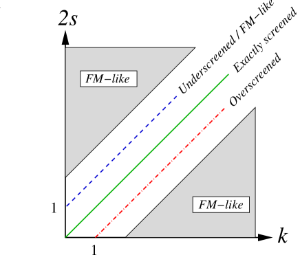
Figure 2: (Color online) Phase diagram of the multichannel Kondo model with $J_{z}\gg|J_{\perp}|,D$, as a function of $k$ and $s$. For $2s=k$ and $2s=k-1$, the low-energy physics is stable against such a large spin-exchange anisotropy. The fixed point remains that of an exactly screened ($2s=k$) or an overscreened ($2s=k-1$) Kondo effect. For $|k-2s|>1$, the low-energy physics is unstable against such a large spin-exchange anisotropy. The system flows to a line of stable ferromagnetic-like fixed points with a residual isospin-$\frac{1}{2}$ local moment. For $2s=k+1$, a large spin-exchange anisotropy is marginal. The system still flows to a line of stable ferromagnetic-like fixed points, however these differ from the isotropic underscreened fixed point only by the marginal operator $\lambda_{z}$ (see text).

(iv) $|k-2s|>1$ — In this effectively underscreened case, the scaling dimension $\Delta_{\perp}$ exceeds one. Hence $\lambda_{\perp}$ is irrelevant, as are all higher order dynamical terms generated within ${\cal H}_{\rm int}$. The system thus flows to a line of stable ferromagnetic-like fixed points, characterized by a finite $\lambda_{z}$ but zero $\lambda_{\perp}$. The low-energy physics is again that of a (potentially singular) Fermi liquid plus a residual isospin $\vec{\tau}$. For $s<k/2-1/2$, this differs markedly from the overscreened fixed point of the isotropic spin-exchange model. Also for $s>k/2+1/2$ this differs from the underscreened fixed point of the isotropic model, as the residual local-moment degeneracy is two instead of $2s-k+1>2$. Importantly, in all cases the resulting low-energy physics is insensitive to the sign of $k-2s$, in stark contrast to the isotropic case. A large spin-exchange anisotropy of the form $J_{z}\gg D,|J_{\perp}|$ is therefore relevant with respect to the isotropic fixed point for all $|k-2s|>1$.

The phase diagram of the multichannel Kondo Hamiltonian with $J_{z}\gg|J_{\perp}|,D$ is summarized in Fig. 2 as a function of $k$ and $s$. Excluding the exactly screened line $2s=k$ and the overscreened line $2s=k-1$, the model flows to a line of stable ferromagnetic-like fixed points with a residual isospin-$\frac{1}{2}$ local moment for all $k$ and $s$. For $2s=k+1$, the ferromagnetic-like fixed points and the isotropic underscreened fixed point are equivalent. They only differ by the marginal operator $\lambda_{z}$. For $2s>k+1$, the ferromagnetic-like fixed points and the isotropic underscreened fixed point are distinctly different, possessing a different residual degeneracy.

VI NRG study of $s=1/2$, $k=3$

Although the strong-coupling expansion unequivocally confirms the existence of a line of stable ferromagnetic-like fixed points for large $J_{z}$ and $|k-2s|>1$, it cannot access the entire phase diagram of the anisotropic multichannel Kondo Hamiltonian. In particular, the second Kosterliz-Thouless line predicted by bosonization for $s=1/2$ and $k>2$ [see Fig. 1(a)] lies beyond the scope of this approach. In this section, we use Wilson’s numerical renormalization-group (NRG) method Wilson75 to conduct a systematic study the phase diagram of the anisotropic multichannel Kondo Hamiltonian with $s=1/2$ and $k=3$.

In conventional formulations of the NRG, Wilson75 one considers a particular choice for the tight-binding parameters in Eq. (39), given by $\epsilon_{j}=0$ and $t_{j}=D_{\Lambda}\Lambda^{-j/2}\xi_{j}$ with

$$D_{\Lambda}=\frac{D}{2}(1+\Lambda^{-1}),$$ (53)

$$\xi_{j}=\frac{1-\Lambda^{-(j+1)}}{\sqrt{(1-\Lambda^{-(2j+1)})(1-\Lambda^{-(2j+3)})}}.$$ (54)

Here $\Lambda>1$ is a discretization parameter. For $\Lambda\to 1^{+}$, the resulting model describes an impurity spin locally coupled to $k$ identical conduction bands with a symmetric box density of states $\rho(E)=(1/2D)\theta(D-|E|)$. For $\Lambda>1$, the model represents an impurity spin coupled to a logarithmically discretized version of the same bands. Wilson75

The first step in the NRG approach is to recast the Hamiltonian ${\cal H}$ as the limit of a sequence of dimensionless Hamiltonians ${\cal H}_{N}$:

$${\cal H}=\lim_{N\rightarrow\infty}\left\{D_{\Lambda}\Lambda^{-(N-1)/2}{\cal H}_{N}\right\}$$ (55)

with

$${\cal H}_{N} = \Lambda^{(N-1)/2}\left[\frac{J_{\perp}}{2D_{\Lambda}}\sum_{n=1}^{k}\left(f^{\dagger}_{0n\downarrow}f_{0n\uparrow}S^{+}+{\rm H.c.}\right)\right.$$

$$+ \frac{J_{z}}{2D_{\Lambda}}\sum_{n=1}^{k}S_{z}\left(f^{\dagger}_{0n\uparrow}f_{0n\uparrow}-f^{\dagger}_{0n\downarrow}f_{0n\downarrow}\right)$$

$$+ \left.\sum_{j=0}^{N-1}\sum_{n=1}^{k}\sum_{\sigma=\uparrow,\downarrow}\Lambda^{-j/2}\xi_{j}\left\{f^{\dagger}_{(j+1)n\sigma}f_{jn\sigma}+{\rm H.c.}\right\}\right].$$

The finite-size Hamiltonians ${\cal H}_{N}$ are then diagonalized iteratively using the NRG transformation

$${\cal H}_{N+1}=\sqrt{\Lambda}{\cal H}_{N}+\sum_{n=1}^{k}\sum_{\sigma=\uparrow,\downarrow}\xi_{N}\left\{f^{\dagger}_{(N+1)n\sigma}f_{Nn\sigma}+{\rm H.c.}\right\}.$$ (57)

Here the prefactor $\Lambda^{(N-1)/2}$ in Eq. (VI) guarantees that the low-energy excitations of ${\cal H}_{N}$ are of order one for all $N$. The approach to a fixed-point Hamiltonian is signaled by a limit cycle of the NRG transformation, with ${\cal H}_{N+2}$ and ${\cal H}_{N}$ sharing the same low-energy spectrum.

It practice, it is impossible to keep track of the exponential increase in the size of the Hilbert space as a function of the chain length $N$. Hence only the lowest $N_{s}$ eigenstates of ${\cal H}_{N}$ are retained at the conclusion of each iteration. comment_on_trunctaion The retained states are used in turn to construct the eigenstates of ${\cal H}_{N+1}$. The truncation error involved can be systematically controlled by varying $N_{s}$. However, since the size of the Hilbert space increases by a factor of $2^{2k}$ with each additional iteration, only a moderately small number of conduction-electron channels can be treated reliably using present-day computers, typically no more than $3$ or $4$ channels. In the following we focus on $k=3$ and $s=1/2$, which is the simplest version of the multichannel Kondo Hamiltonian that is both amendable to the NRG and predicted to display the phase diagram of Fig. 1(a).

To cope with the large computational effort involved in exploring the phase diagram of the three-channel Kondo model with spin-exchange anisotropy, we used rather large values of $\Lambda$ (either $\Lambda=3$ or $\Lambda=5$), and applied an alternative truncation scheme to the one customarily used. Since each of the NRG Hamiltonians ${\cal H}_{N}$ is block diagonal in the conserved quantum numbers, comment_on_conserved_numbers the computational time is mostly governed by the largest block to be diagonalized. Thus, instead of retaining a fixed number of eigenstates of ${\cal H}_{N}$, at each iteration we adjusted the threshold energy for truncation so that the largest block did not exceed $N_{\rm block}$ states. comment_on_trunctaion For $\Lambda=3$ we used $N_{\rm block}=100$, while for $\Lambda=5$ we set $N_{\rm block}=80$. This approach gave rise to variations in the number of states retained at the conclusion of each iteration. Typically, 3000 to 4000 states were retained. In some extreme cases down to 2500 states and up to 5500 states were kept. We have verified that the threshold energies selected in this way were sufficiently high so as not to spoil the accuracy of the calculations.

Figure 3 depicts the finite-size spectra obtained for $\rho J_{\perp}=0.008$ and different values of $\rho J_{z}>0$. Here $\Lambda=3$ was used. Up to a critical coupling $\rho J_{z}^{c}\approx 1.26$, the system always flows to the non-Fermi-liquid fixed point of the three-channel Kondo effect. Indeed, the fixed-point spectrum is independent of $J_{z}<J_{z}^{c}$, and is identical to that for isotropic spin-exchange interaction (left-most panel). There is excellent agreement with the finite-size spectrum of the three-channel Kondo effect obtained from conformal field theory, AL91 whose energy levels are marked by arrows in Fig. 3. Here the slight splitting of NRG levels near the dimensionless energy $1.6$ is a $\Lambda$-dependent feature. This splitting is reduced upon decreasing $\Lambda$, and should disappear for $\Lambda\to 1^{+}$.

A different picture is recovered for $J_{z}>J_{z}^{c}$. (i) As demonstrated in Fig. 3 for $\rho J_{z}=1.36$ and $\rho J_{z}=6.4$, the finite-size spectrum remains Fermi-liquid-like down to the lowest energies reached ($E\sim 10^{-120}D$ in some extreme runs), without crossing over to the overscreened fixed point of the three-channel Kondo effect. (ii) The finite-size spectrum varies continuously with $J_{z}>J_{z}^{c}$, suggesting the flow to a line of fixed points connected by a marginal operator. (iii) For $J_{z}\gg J_{z}^{c}$, the quantum numbers and degeneracies of the NRG levels are in excellent agreement with those anticipated based on the strong-coupling analysis of Sec. IV. (iv) The NRG level flow confirms that channel asymmetry is a marginal perturbation for $J_{z}>J_{z}^{c}$ (not shown), in stark contrast to the regime $J_{z}<J_{z}^{c}$. These features are all consistent with the flow to a line of stable ferromagnetic-like fixed points as predicted by bosonization.

Figure 3: NRG level flow (odd iterations) for $s=1/2$, $k=3$, $\rho J_{\perp}=0.008$, and increasing values of $\rho J_{z}$. Here $\Lambda=3$ was used. For $\rho J_{z}<\rho J_{z}^{c}\approx 1.26$ (left two panels), the system flows to the non-Fermi-liquid fixed point of the three-channel Kondo effect, irrespective of $J_{z}$. There is excellent agreement with the finite-size spectrum of three-channel Kondo effect obtained from conformal field theory, whose energy levels (in units of the fundamental level spacing) are indicated by arrows. For $J_{z}>J_{z}^{c}$ (right two panels), the finite-size spectrum remains Fermi-liquid-like down to minuscule energies, without crossing over to the non-Fermi-liquid fixed point of the three-channel Kondo effect. The persisting drift of NRG levels for $J_{z}>J_{z}^{c}$ appears to be due to some weak numerical instability. A similar drift of levels occurs for $-J_{z}\gg J_{\perp}>0$ (ferromagnetic coupling).

We do note, however, a persisting drift of the NRG levels for $J_{z}>J_{z}^{c}$. A similar drift of levels occurred for $-J_{z}\gg|J_{\perp}|>0$ (ferromagnetic coupling), and appears to be driven by some weak numerical instability. While we cannot entirely rule out an eventual crossover to the non-Fermi-liquid fixed point of the three-channel Kondo effect at some lower temperature, we find this scenario highly unlikely given the extremely low energy scales reached and the rapid change of behavior as $J_{z}$ is swept through $J_{z}^{c}$. We therefore identify $J_{z}^{c}$ with the phase boundary between the antiferromagnetic and the new ferromagnetic-like domain predicted by bosonization.

Guided by this interpretation, we turned to explore the dependence of $J_{z}^{c}$ on $J_{\perp}$. The resulting phase diagram is plotted in Fig. 4, for $\Lambda=5$. While points on the solid line all converged to the non-Fermi-liquid fixed point of the three-channel Kondo effect, points on the dashed line showed no such tendency up to $N=120$ NRG iterations (corresponding to $E\sim 10^{-42}D$). We therefore estimate the phase boundary between the antiferromagnetic and the ferromagnetic-like domains to lie in between the solid and dashed lines. In contrast to the solid line, which definitely lies on the antiferromagnetic side of the transition, one cannot guarantee that all points on the dashed line lie on the ferromagnetic-like side. We have confirmed, however, that the phase diagram of Fig. 4 is practically unchanged upon going to $N=180$ iterations. We further stress that the exact position of the phase boundary is in general $\Lambda$ dependent, although its dependence on $\Lambda$ appears to be weak. For $\Lambda=3$, for example, the position of the phase boundary varied by no more than just a few percent. We expect a similar proximity of the $\Lambda\to 1^{+}$ phase boundary.

Figure 4: NRG phase boundary between the antiferromagnetic and the new ferromagnetic-like domain, for $s=1/2$, $k=3$ and $\Lambda=5$. Points on the solid line all converged to the non-Fermi-liquid fixed point of the three-channel Kondo effect. Points on the dashed line showed no such tendency up to $N=120$ NRG iterations, corresponding to $E\sim 10^{-42}D$. We estimate the phase boundary between the two domains to lie in between the solid and dashed lines.

The above results are clearly in good qualitative agreement with the bosonization treatment of Sec. III. We now turn to a more quantitative comparison. Setting $k=3$ in Eq. (37), the critical coupling $J_{z}^{\ast}$ predicted by bosonization is equal to $\rho J_{z}^{\ast}=4\sqrt{3}/\pi\approx 2.2$. Based on the NRG results for $\Lambda=3$ and $\Lambda=5$, we estimate the location of the critical coupling for a symmetric box density of states (i.e., for $\Lambda\to 1^{+}$) to be around $\rho J_{z}^{\ast}\sim 1.2-1.3$. Thus, the bosonization and NRG results are within a factor of two from one another. Considering that $J_{z}^{\ast}$ lies well beyond the strict range of validity of bosonization, we find this degree of agreement to be quite remarkable. As for the shape of the phase boundary, it was predicted in Sec. III to have the linear form $J_{z}=J_{z}^{\ast}+C_{k}|J_{\perp}|$, where $0<C_{k}<1$ is given by Eq. (38). As seen in Fig. 4, the NRG phase boundary for $\Lambda=5$ is well described by a linear curve, at least up to $\rho J_{\perp}\approx 0.08$. The corresponding slope $C_{\rm NRG}\approx 0.67$ is indeed less than one, but is nearly three-fold larger than the bosonization result, $C_{k=3}=0.25$. This discrepancy can be largely accounted for by plugging the NRG value for $\rho J_{z}^{\ast}$ into the right-hand side of Eq. (38), which yields $C\approx 0.5$.

VII Discussion and summary

The multichannel Kondo Hamiltonian is an important paradigm in correlated electron systems, with possible applications to varied systems. Depending on the size of the impurity spin, $s$, and the number of independent conduction-electron channels, $k$, it can display either local Fermi-liquid, singular Fermi-liquid, or non-Fermi-liquid behavior. Although the isotropic model is by now well understood, we have shown in this paper that an XXZ spin-exchange anisotropy has a far more elaborate effect on its low-energy physics than previously appreciated. Below we briefly summarize our main findings and discuss their implications. A detailed account of our results is presented in Fig. 1.

We begin with a spin-$\frac{1}{2}$ impurity and with $k>2$ conduction-electron channels. From conformal field theory it is known that the non-Fermi-liquid fixed point of the corresponding Kondo model is stable against a small spin-exchange anisotropy. ALPC92 However, it was found to be unstable against a sufficiently large $J_{z}\gg|J_{\perp}|>0$. In the latter regime, the system flows to a line of stable ferromagnetic-like fixed points with a residual isospin-$\frac{1}{2}$ local moment. The phase diagram of the model thus consists of three distinct domains: the conventional ferromagnetic and antiferromagnetic (i.e., non-Fermi-liquid) domains, plus a second ferromagnetic-like domain located deep in the antiferromagnetic regime. The new ferromagnetic-like domain extends above a critical longitudinal coupling $J_{z}^{\ast}$, whose magnitude depends on $k$. While $J_{z}^{\ast}$ exceeds the bandwidth for intermediate values of $k$, it is pushed to weak coupling for $k\gg 1$. Each of the two ferromagnetic-type domains is separated from the antiferromagnetic one by a Kosterliz-Thouless line, as depicted in Fig. 1(a). While we cannot entirely rule out the possibility of yet another domain for sufficiently large $|J_{\perp}|\gg J_{z}$, there are no indications at this point in favor of such a scenario.

Proceeding to $1/2<s<k/2-1/2$, spin-exchange anisotropy is known ALPC92 to be a relevant perturbation at the overscreened non-Fermi-liquid fixed point for $k>4$ (for $k=4$ it is a marginal perturbation). The basin of attraction of the overscreened fixed point is therefore confined to the line $J_{z}=|J_{\perp}|>0$. The nature of the low-temperature fixed points for $J_{z}\neq|J_{\perp}|$ was never explored. As shown in Secs. II and V, the system flows to a line of stable ferromagnetic-like fixed points with a residual isospin-$\frac{1}{2}$ local moment both for sufficiently small $J_{z}>|J_{\perp}|$ (i.e., in the limit $J_{z},J_{\perp}\to 0$ for any given ratio $J_{z}/|J_{\perp}|>1$) and for a sufficiently large $J_{z}\gg|J_{\perp}|>0$. This suggests a single generic behavior in the entire domain $J_{z}>|J_{\perp}|$. Further support in favor of this interpretation is provided in Appendix A, for the special case of a spin-one impurity. As for the domain $|J_{z}|<|J_{\perp}|$, here information is confined to the weak-coupling regime, $|\rho J_{\perp}|\ll 1/ks$. Depending on the parity of $2s$, the system flows either to a conventional Fermi liquid with no residual degeneracy (integer $s$), or to a $k$-channel Kondo effect with an effective spin-$\frac{1}{2}$ local moment (half-integer $s$). It remains to be seen to what extent is this behavior generic to $|J_{z}|<|J_{\perp}|$.

For isotropic antiferromagnetic exchange and $k>2$, the two overscreened spins $s=1/2$ and $s=k/2-1/2$ share the same low-energy physics. Indeed, the corresponding Kondo models are related for $J_{z}=J_{\perp}>0$ through a weak-to-strong-coupling duality. It is not surprising, then, that the overscreened fixed point shows the same stability for both spins against a weak spin-exchange anisotropy. ALPC92 A similar duality appears to hold also for an XXZ anisotropy, at least in the range $J_{z}>|J_{\perp}|$. Indeed, for $s=1/2$ the overscreened fixed point is stable at weak coupling (assuming $J_{z}>-|J_{\perp}|$), giving way to a line of stable ferromagnetic-like fixed points for sufficiently large $J_{z}\gg|J_{\perp}|>0$. For $s=k/2-1/2$ the roles are reversed. The overscreened fixed point is stable against a sufficiently large $J_{z}\gg|J_{\perp}|>0$, but is unstable for sufficiently small $J_{z}>|J_{\perp}|$. In the latter regime, the system flows to the same line of stable ferromagnetic-like fixed points that is approached for $s=1/2$ and a large $J_{z}$. Note that, for $s=k/2-1/2$ and small $|J_{\perp}|>|J_{z}|$, the stability of the overscreened fixed point depends on the parity of $k$. The overscreened fixed point is stable for half-integer $s$ (even $k$), but is unstable for integer $s$ (odd $k$).

All cases discussed above pertain to an overscreened impurity. We now turn to an underscreened spin, i.e., $s>k/2$. As shown in Secs. II and V, an XXZ anisotropy is a relevant perturbation both near the free-impurity fixed point and for a sufficiently large $J_{z}\gg|J_{\perp}|$. The sole exception to the rule is the case $s=k/2+1/2$, where $\delta J=J_{z}-|J_{\perp}|>0$ is a marginal perturbation in each of these limits. Consider first the range $J_{z}>|J_{\perp}|$. Here the flow in both extremes is to the same line of ferromagnetic-like fixed points with a residual isospin-$\frac{1}{2}$ local moment. As before, this suggests a single generic behavior throughout the domain $J_{z}>|J_{\perp}|$. Similar to the case of isotropic antiferromagnetic exchange, the low-energy physics is comprised of quasiparticle excitations plus a residual local moment. However, the residual degeneracy for $s>k/2+1/2$ is smaller than that of the isotropic underscreened fixed point (two versus $2s-k+1>2$), distinguishing the ferromagnetic-like line of fixed points from the isotropic underscreened one.

Of the different possible cases, the most intriguing perhaps is that of an underscreened impurity with $|J_{z}|<|J_{\perp}|$ and half-integer $s$. As we have shown in Sec. II, the resulting low-energy physics is that of a $k$-channel, spin-$\frac{1}{2}$ Kondo effect, at least in the limit of sufficiently weak coupling. Thus, an XXZ anisotropy drives the system from underscreened to overscreened behavior. A more complete characterization of the transition between these two distinctly different behaviors is clearly needed.

Going back to $s=1/2$, we conclude with a few further comments on the mapping of Eq. (1). We first reiterate that $J_{z}^{\ast}$ lies well beyond the strict range of validity of bosonization for intermediate values of $k$. Nevertheless, this approach (and its Anderson-Yuval equivalent Ye96 ) well describes the new ferromagnetic-like phase both qualitatively and quantitatively. For $k=3$, which features the largest $J_{z}^{\ast}$ and is thus the most prone to error, Eq. (37) is only a factor of two larger than the NRG estimate for a symmetric box density of states. We find this degree of quantitative agreement to be quite remarkable.

Although the mapping of Eq. (1) was derived in Sec. III for a channel-isotropic model, it can easily be extended to channel anisotropy both in the spin-flip coupling, $J_{\perp}\to J_{\perp n}$, and in the longitudinal coupling, $J_{z}\to J_{zn}$. The individual transverse couplings remain unchanged in the course of the mapping, whether isotropic or not. As for the individual longitudinal couplings, these transform according to

$$\arctan\left(\frac{\pi\rho J^{\prime}_{zn}}{4}\right)=\frac{\pi}{k}+\arctan\left(\frac{\pi\rho J_{zn}}{4}\right)-2\bar{\delta}_{z},$$ (58)

where

$$\bar{\delta}_{z}=\frac{1}{k}\sum_{n=1}^{k}\arctan\left(\frac{\pi\rho J_{zn}}{4}\right)$$ (59)

is the average phase shift for the $k$ different channels. Accordingly, the mapping of Eqs. (58) and (59) is restricted to values of $J_{zn}$ where the modulus of the right-hand side of Eq. (58) does not exceed $\pi/2$ for any of the $k$ channels. Observe that channel anisotropy is preserved by Eqs. (58) and (59), which adequately reduce to Eq. (1) in the limit of isotropic couplings.

Finally, we remark on the possibility of generalizing the mapping of Eq. (1) to arbitrary spin $s$. Two modifications appear when the same sequence of steps is applied to an impurity spin larger than one-half: (i) For $s>1$, the phase shift $\delta_{z}$ in the absence of $J_{\perp}$ is a nonlinear function of $S_{z}$. Hence, the bosonized form of the $J_{z}$ interaction term is no longer linear in $S_{z}$ as for $s=1/2$. (ii) The unitary transformation $U$ produces an additional Hamiltonian term of the form $\Delta S_{z}^{2}$, similar to the one generated in perturbative RG [see Eq. (12)]. For $s=1/2$, this term amounts to a uniform shift of the entire spectrum, which can be safely ignored. This, however, is no longer the case for $s>1/2$, where different Kramers doublets are split. As a result of the former modification, the mapped Hamiltonian no longer assumes the form of a simple spin-exchange Hamiltonian for $s>1$. The case $s=1$ is an exception in this regard. The mapped Hamiltonian does acquire an additional $\Delta S_{z}^{2}$ term, but otherwise retains the form of a conventional spin-exchange interaction. A detailed discussion of this particular case is presented in Appendix A.

Appendix A Exact mapping for $s=1$

In this appendix, we extend the mapping of Eq. (1) to a spin-one impurity. As explained in the main text, $s=1$ is the only other spin size for which a simple spin-exchange interaction is restored at the conclusion of the mapping. However, an additional local field proportional to $S_{z}^{2}$ is generated. The basic steps of the derivation are nearly identical to those carried out in Sec. III for $s=1/2$. Only a few minor modifications appear, as specified below.

Our starting point is the Hamiltonian of Eq. (III), where $\vec{S}$ now represents a spin-one operator. Bosonizing the fermion fields according to Eq. (20), the bosonic Hamiltonian assumes the form of Eq. (23) with one sole variation: The longitudinal spin-exchange term now reads

$$\delta_{1}\frac{a}{2\pi^{2}\rho}\sum_{n=1}^{k}\left[\nabla\Phi_{n\uparrow}(0)-\nabla\Phi_{n\downarrow}(0)\right]S_{z},$$ (60)

where

$$\delta_{1}=\arctan\left(\frac{\pi\rho J_{z}}{2}\right).$$ (61)

Converting to the boson fields of Eqs. (25) and (26) and applying the transformation $U=\exp\left[i\sqrt{\frac{8}{k}}\Phi_{s}(0)S_{z}\right]$, the transformed Hamiltonian ${\cal H}^{\prime}=U{\cal H}U^{\dagger}$ retains the same overall form as Eq. (31), but with two important modifications: (i) The coefficient of the $\nabla\Phi_{s}(0)S_{z}$ term is replaced with

$$\left(\delta_{1}-\frac{2\pi}{k}\right)\frac{a}{2\pi^{2}\rho}\sqrt{2k}\;;$$ (62)

(ii) A new Hamiltonian term ${\cal H}_{\Delta}=\Delta S_{z}^{2}$ with

$$\Delta=8D\left[\frac{1}{k}-\frac{\delta_{1}}{\pi}\right]$$ (63)

is added to ${\cal H}^{\prime}$. comment_on_delta Proceeding with the transformation $\Phi_{s}(x)\to-\Phi_{s}(x)$ and converting back to a fermionic representation, the Hamiltonian ${\cal H}^{\prime}$ regains the form of Eq. (III), but with certain renormalized parameters:

$$J_{z}\to J^{\prime}_{z},$$ (64)

$$h\to-h,$$ (65)

$$g_{i}\to 2g_{e}-g_{i},$$ (66)

and

$$\Delta=0\to 8D\left[\frac{1}{k}-\frac{\delta_{1}}{\pi}\right].$$ (67)

Here $J^{\prime}_{z}$ is determined from the equation

$$\arctan\left(\frac{\pi\rho J^{\prime}_{z}}{2}\right)=\frac{2\pi}{k}-\arctan\left(\frac{\pi\rho J_{z}}{2}\right),$$ (68)

which comes in place of Eq. (1) for a spin-$\frac{1}{2}$ impurity.

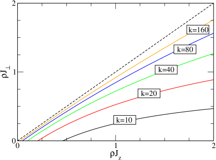
Figure 5: (Color online) Lower bound on the basin of attraction of the line of stable ferromagnetic-like fixed points, for $s=1$ and different values of $k\gg 1$. In the region below and to the right of each solid line, both $\Delta<0$ and $J^{\prime}_{z}<-|J_{\perp}|$. Hence the system flows to the line of stable ferromagnetic-like fixed points with a residual degeneracy of two. The fixed-point structure in the remaining portion of the domain $J_{z}>|J_{\perp}|$, i.e., in between the solid lines and the overscreened line $J_{z}=|J_{\perp}|$ (marked by a dashed line), cannot be deduced based on Eqs. (64)–(68) alone.

As for $s=1/2$, the mapping of Eqs. (64)–(68) is restricted to values of $J_{z}$ where the right-hand side of Eq. (68) does not exceed $\pi/2$. This constrains the mapping to $k\geq 3$ (overscreened impurity), and to $J_{z}\geq J_{\rm min}$ with

$$J_{\rm min}=\left\{\begin{array}[]{lcc}\frac{2}{\sqrt{3}\pi\rho}>0&&k=3\\ \\ 0&&k=4\\ \\ -\frac{2}{\pi\rho}\tan\left(\frac{\pi}{2}-\frac{2\pi}{k}\right)<0&&k>4\end{array}\;\;.\right.$$ (69)

Specifically, for $k>4$ the coupling regimes $J_{\rm min}\leq J^{\prime}_{z}<0$ and $J_{z}>J_{z}^{\ast}>0$ with

$$J_{z}^{\ast}=\frac{2}{\pi\rho}\tan\left(\frac{2\pi}{k}\right)$$ (70)

are mapped onto one another. This should be compared with Eqs. (36) and (37) for $s=1/2$.

Since Eqs. (64)–(68) define yet another multichannel Kondo Hamiltonian with both spin-exchange anisotropy and a potentially competing $\Delta S_{z}^{2}$ term, we have no conclusive way to deduce its fixed-point structure throughout the $J_{z}$–$J_{\perp}$ plane. Nevertheless, the behavior in one particular region is clear. For values of $J_{z}$ where both $J_{z}^{\prime}<-|J_{\perp}|$ and $\Delta<0$, the spin-exchange interaction and the $\Delta S_{z}^{2}$ term conspire to favor a ferromagnetic-like state with two-fold residual degeneracy. Here the residual degeneracy originates from the $S_{z}^{2}=1$ Kramers doublet favored by $\Delta<0$. For such values of $J_{z}$, one can safely conclude that the system flows to the line of stable ferromagnetic-like fixed points identified previously from the strong-coupling expansion of Sec. V. These considerations provide us with the following lower bound on the basin of attraction of the ferromagnetic-like line of fixed points:

$$|J_{\perp}|<|J_{\rm min}|,$$ (71)

$$J_{z}>\frac{2}{\pi\rho}\tan\left[\frac{2\pi}{k}+\arctan\left(\frac{\pi\rho|J_{\perp}|}{2}\right)\right].$$ (72)

Figure 5 depicts that portion of the $J_{z}$–$J_{\perp}$ plane defined by Eqs. (71) and (72), for several values of $k\gg 1$. With increasing $k$, a growing fraction of the domain $J_{z}>|J_{\perp}|$ is covered by this region, which stretches for $k\gg 1$ from $\rho J_{z}\approx 4/k\ll 1$ and upward in $J_{z}$. This result partially bridges between the strong- and weak-coupling limits ($\rho J_{z}\gg 1,|\rho J_{\perp}|$ and $0<|\rho J_{\perp}|<\rho J_{z}\ll 1/k$, respectively), where flow to a ferromagnetic-like state has been established in Secs. II and V using vastly different techniques. As for the remaining fraction of the domain $J_{z}>|J_{\perp}|$, its fixed-point structure cannot be immediately deduced based on Eqs. (64)–(68) alone.

References

- (1) D. L. Cox, Phys. Rev. Lett. 59, 1240 (1987).
- (2) C. L. Seaman, M. B. Maple, B. W. Lee, S. Ghamaty, M. S. Torikachvili, J.-S. Kang, L. Z. Liu, J. W. Allen, and D. L. Cox, Phys. Rev. Lett. 67, 2882 (1991).
- (3) D. C. Ralph and R. A. Buhrman, Phys. Rev. Lett. 69, 2118 (1992).
- (4) D. C. Ralph, A. W. W. Ludwig, J. von Delft and R. A. Buhrman, Phys. Rev. Lett. 72, 1064 (1994).
- (5) A. Zawadowski, Phys. Rev. Lett. 45, 211 (1980).
- (6) K. Vladar and A. Zawadowski, Phys. Rev. B 28, 1564 (1983); 28 1582 (1983); 28 1596 (1983).
- (7) T. Cichorek, A. Sanchez, P. Gegenwart, F. Weickert, A. Wojakowski, Z. Henkie, G. Auffermann, S. Paschen, R. Kniep, and F. Steglich, Phys. Rev. Lett. 94, 236603 (2005). This paper reports two-channel Kondo characteristics in transport properties of ThAsSe, presumably due to scattering off structural two-level systems.
- (8) K. A. Matveev, Zh. Eksp. Teor. Fiz. 99, 1598 (1991) [Sov. Phys. JETP 72, 892 (1991)].
- (9) D. Berman, N. B. Zhitenev, R. C. Ashoori, and M. Shayegan, Phys. Rev. Lett. 82, 161 (1999).
- (10) For a comprehensive review of the multichannel Kondo effect, see D. L. Cox and A. Zawadovski, Adv. Phys. 47, 599 (1998).
- (11) A. Posazhennikova and P. Coleman, Phys. Rev. Lett. 94, 036802 (2005).
- (12) P. Mehta, N. Andrei, P. Coleman, L. Borda, and G. Zaránd, Phys. Rev. B 72, 014430 (2005).
- (13) P. Coleman and C. Pépin, Phys. Rev. B 68, 220405(R) (2003).
- (14) W. Koller, A. C. Hewson, and D. Meyer, Phys. Rev. B 72, 045117 (2005).
- (15) I. Affleck, A. W. W. Ludwig, H.-B. Pang, and D. L. Cox, Phys. Rev. B 45, 7918 (1992).
- (16) K. G. Wilson, Rev. Mod. Phys. 47, 773 (1975).
- (17) M. Fabrizio, A. O. Gogolin, and P. Noziéres, Phys. Rev. B 51, 16088 (1995).
- (18) J. Ye, Phys. Rev. Lett. 77, 3224 (1996).
- (19) P. W. Anderson, J. Phys. C 3, 2436 (1970).
- (20) F. D. M. Haldane, J. Phys. C 14, 2585 (1981).
- (21) P. Noziéres and A. Blandin, J. Physique 41, 193 (1980).
- (22) See Eqs. (2) of Ref.Ye96, with .
- (23) Careless truncation may result in spurious symmetry breaking. To avoid symmetry breaking in the course of truncation it is essential to accommodate the degenerate multiplets of in their entirety. This may require a slight increase in the number of states retained at certain iterations.
- (24) In our code we exploited the conservation of the following quantities: the total electronic charge, the component of the overall spin of the system, and the operator . We did not make use of the full SU(3) channel symmetry of the model.
- (25) I. Affleck, A. W. W. Ludwig, Nucl. Phys. B360, 641 (1991).
- (26) is formally proportional to , which is regularized as .