Strong correlations in low dimensional systems

Abstract

I describe in these notes the physical properties of one dimensional interacting quantum particles. In one dimension the combined effects of interactions and quantum fluctuations lead to a radically new physics quite different from the one existing in the higher dimensional world. Although the general physics and concepts are presented, I focuss in these notes on the properties of interacting bosons, with a special emphasis on cold atomic physics in optical lattices. The method of bosonization used to tackle such problems is presented. It is then used to solve two fundamental problems. The first one is the action of a periodic potential, leading to a superfluid to (Mott)-Insulator transition. The second is the action of a random potential that transforms the superfluid in phase localized by disorder, the Bose glass. Some discussion of other interesting extensions of these studies is given.

1 Introduction and choice of contents

One-dimensional systems of interacting particles are particularly fascinating both from a theoretical and experimental point of view. Such systems have been extensively investigated theoretically for more than 40 years now. They are wonderful systems in which interactions play a very special role and whose physics is drastically different from the ‘normal’ physics of interacting particles, that is, the one known in higher dimensions. From the theoretical point of view they present quite unique features. The one-dimensional character makes the problem simple enough so that some rather complete solutions could be obtained using specific methods, and yet complex enough to lead to incredibly rich physics Emery (1979); Sólyom (1979); Voit (1995); Schulz (1995); von Delft and Schoeller (1998); Schönhammer (2002); Senechal (2003); Gogolin et al. (1999); Giamarchi (2004a).

Crucial theoretical progress were made and many theoretical tools got developed, mostly in the 1970’s allowing a detailed understanding of the properties of such systems. This culminated in the 1980’s with a new concept of interacting one-dimensional particles, analogous to the Fermi liquid for interacting electrons in three dimensions: the Luttinger liquid. Since then many developments have enriched further our understanding of such systems, ranging from conformal field theory to important progress in the exact solutions such as Bethe ansatz Takahashi (1999).

In addition to these important theoretical progress, experimental realizations have knows comparably spectacular developments. One-dimensional systems were mostly at the beginning a theorist’s toy. Experimental realizations started to appear in the 1970’s with polymers and organic compounds. But in the last 20 years or so we have seen a real explosion of realization of one-dimensional systems. The progress in material research made it possible to realize bulk materials with one-dimensional structures inside. The most famous ones are the organic superconductors rev (2004) and the spin and ladder compounds Dagotto and Rice (1996). At the same time, the tremendous progress in nanotechnology allowed to obtain realizations of isolated one-dimensional systems such as quantum wires Fisher and Glazman (1997), Josephson junction arrays Fazio and van der Zant (2001), edge states in quantum hall systems Wen (1995), and nanotubes Dresselhaus et al. (1995). Last but not least, the recent progress in Bose condensation in optical traps have allowed an unprecedented way to probe for strong interaction effects in such systems Pitaevskii and Stringari (2003); Greiner et al. (2002).

The goal of these lectures was therefore to present the major theoretical tools of the domain. However, while writing these notes, I was faced with a dilemma. Having written a recent book on this very subject Giamarchi (2004a) it felt that writing these notes would be a simple repetition or worse a butchering of the explanations that could be found in the book. I have thus chosen to give to these notes a slightly different focuss than the material that was actually presented during the course. For an introduction to the one dimensional systems and in particular for the fermionic problems, as well as most of the technical details, I refer the reader to Giamarchi (2004a) where all this material is described in detail and hopefully in a pedagogical fashion suitable for graduate students. I have chosen to restrict these notes to the description of one and quasi-one dimensional systems of bosons. Indeed the spectacular recent progress made thanks to cold atomic gases, make it useful to have a short summary on the subject, in complement of the material that can already be found in Giamarchi (2004a). Note that although these notes do cover some of the basic material for cold atoms they cannot pretend to be an exhaustive and complete review on this rapidly developing subject. The whole volume of this book would not be sufficient for that. Rather they reflect a partial selection, based on my own excitement in the field and its connections with the low dimensional world. I thus apologize in advance for those whose pet theory, experiment or paper I would fail to mention in these notes.

2 One dimensional bosons, and their peculiarities

Bosons are particularly interesting systems to investigate. From the theoretical point of view bosons present quite interesting peculiarities and are in fact a priori much more difficult to treat than their fermionic counterpart. Indeed, for fermions, the free fermion approximation is usually a good starting point, at least in high enough dimension where Fermi liquid theory holds. Some perturbations such as disorder can be studied for the much simpler free fermion case, the Pauli principle ensuring that even in the absence of interactions the perturbation remains small compared to the characteristic scales of the free problem (here the Fermi energy). One can thus gain valuable physical intuition on the problem before adding the interactions. For bosons, on the contrary, interactions are needed from the start since there are radical differences between a non-interacting boson gas and an interacting one. Bosons have another remarkable property, namely in the absence of interactions all the particles can condense in a macroscopic state. Interacting bosons thus constitute a remarkable theoretical challenge. One dimension presents additional peculiarities as we will see below.

Before embarking on the subject of interacting bosons, let us first discuss how one can obtain “one dimensional” objects. Of course the real world is three dimensional, but all the one dimensional system are characterized by a confining potential forcing the particles to be in a localized states

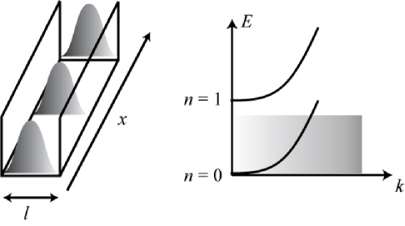
Figure 1: (left) Confinement of the electron gas in a one-dimensional tube of transverse size $l$. $x$ is the direction of the tube. Only one transverse direction of confinement has been shown for clarity. Due to the transverse confining potential the transverse degrees of freedom are strongly quantized. (right) Dispersion relation $E(k)$. Only half of the dispersion relation is shown for clarity. $k$ is the momentum parallel to the tube direction. The degrees of freedom transverse to the tube direction lead to the formation of minibands, labelled by a quantum number $n$. One can be in a situation where only one miniband can be excited, due to temperature or interactions, the energy scale of which is represented by the gray box. In that case the system is equivalent to a one dimensional system where only longitudinal degrees of freedom can vary.

The wavefunction of the system is thus of the form

$$\psi(x,y)=e^{ikx}\phi(y)$$ (1)

where $\phi$ depends on the precise form of the confining potential For an infinite well, a show in Fig. 1, $\phi$ is $\phi(y)=\sin((2n_{y}+1)\pi y/l)$, whereas it would be a gaussian function (8) for an harmonic confinement. The energy is of the form

$$E=\frac{k^{2}}{2m}+\frac{k_{y}^{2}}{2m}$$ (2)

where for simplicity I have taken hard walls confinement. The important point is the fact that due to the narrowness of the transverse channel $l$, the quantization of $k_{y}$ is sizeable. Indeed, the change in energy by changing the transverse quantum number $n_{y}$ is at least (e.g. $n_{y}=0$ to $n_{y}=1$)

$$\Delta E=\frac{3\pi^{2}}{2ml^{2}}$$ (3)

This leads to minibands as shown in Fig. 1. If the distance between the minibands is larger than the temperature or interactions energy one is in a situation where only one miniband can be excited. The transverse degrees of freedom are thus frozen and only $k$ matters. The system is a one-dimensional quantum system.

We can thus forget about the transverse directions and model the bosons keeping only the longitudinal degrees of freedom. Two slightly different starting points are possible. One can start directly in the continuum, where bosons are described by

$$H=\int dx\frac{\hbar^{2}(\nabla\psi)^{\dagger}(\nabla\psi)}{2m}+\frac{1}{2}\int dx\;dx^{\prime}\;V(x-x^{\prime})\rho(x)\rho(x^{\prime})-\mu_{0}\int dx\;\rho(x)$$ (4)

The first term is the kinetic energy, the second term is the repulsion $V$ between the bosons and the last term is the chemical potential. A famous model, exactly solvable by Bethe-ansatz Lieb and Liniger (1963) uses a local repulsion

$$V(x)=V_{0}\delta(x)$$ (5)

Note that $V$ is not the real atom-atom interaction in three dimensional space but an effective interaction where the transverse degrees of freedom have already been incorporated. The extension of the transverse wavefunction is of course much larger than the dimensions of the atoms themselves, so the hard core repulsion between two atoms can be safely forgotten. The three dimensional interaction is characterized by a scattering length Pitaevskii and Stringari (2003) $a_{s}$ by

$$V(x,y,z)=\frac{4\pi\hbar^{2}a_{s}}{m}\delta(x)\delta(y)\delta(z)$$ (6)

Note that for bosons the s-wave scattering is the important one since two bosons can get close together due to the symmetry of their wave function, while for fermions this scattering would be highly inefficient. $V_{0}$ in (5) is obtained by integrating over the transverse degrees of freedom of the wavefunction. Because the effective interaction depends on the extension of the transverse wavefunction it will be possible to vary (increase) it by increasing the confinement Olshanii (1998). To be closer to the situation for cold atomic gases one has to remember that there is also a confining potential in the longitudinal direction even if this one is much more shallow and therefore the chemical potential is spatially dependent, leading to a term of the form

$$H=\int dx[V_{c}(x)-\mu_{0}]\rho(x)$$ (7)

where $\mu(x)=\frac{1}{2}m\omega_{0}^{2}x^{2}$ is the confining potential. In the absence of interactions the ground state of the system is given by an harmonic oscillator wavefunction

$$\psi_{0}(x)=\left(\frac{m\omega_{0}}{\hbar\pi}\right)^{1/4}e^{-\frac{m\omega_{0}}{2\hbar}x^{2}}$$ (8)

In the absence of the confining potential the bosons are in a plane wave state of momentum $k=0$, whereas here they are confined on a typical length of order $a_{K}=\sqrt{\hbar/(m\omega_{0})}$ in presence of the harmonic potential. A similar but much tighter confinement is imposed in the transverse directions as well, leading to the formation of the tubes as discussed above. Typical longitudinal lengths due to the harmonic confinement are $15\mu m$ while the transverse dimensions can be $60nm$ Stöferle et al. (2004); Kinoshita et al. (2004); Paredes et al. (2004).

Due to the trap the density profile is thus non homogeneous. In the absence of interactions it would just be the gaussian profile of (8). In presence of interactions a similar effect occurs but the profile changes. A very simple way to see this effect is when one can neglect the kinetic energy (so called Thomas-Fermi approximation; for other situations see Pitaevskii and Stringari (2003)). In that case the density profile is obtained by minimizing (4) and (7), leading to

$$V_{0}\rho(x)+[V_{c}(x)-\mu_{0}]=0$$ (9)

the density profile is thus an inverted parabola, reflecting the change of the chemical potential. One can express the confining length as $a=a_{K}\sqrt{(2\rho_{0}V_{0})/(\hbar\omega_{0})}$ where $\rho_{0}$ is the density at the center of the trap. Of course dealing with such inhomogeneous system is a complication and has consequences that I will discuss below. To treat this problem, there are various approximations that one can make. The crudest way of dealing with such a confinement is simply to ignore the spatial variation and remember the trap as giving a finite size to the system.

In the model (4), the bosons move in a continuum. It is interesting to add to the system (4) a periodic potential $V_{L}(x)$ coupled to the density Jaksch et al. (1998); Greiner et al. (2002); Stöferle et al. (2004)

$$H_{L}=\int dx\;V_{L}(x)\rho(x)$$ (10)

This term, which favors certain points in space for the position of the bosons, mimics the presence of a lattice of period $a$, the periodicity of the potential $V_{L}(x)$. We take the potential as

$$V_{L}(x)=V_{L}\sin^{2}(kx)=\frac{V_{L}}{2}[1-\cos(2kx)]$$ (11)

one has thus $a=\pi/k$. The presence of the lattice can drastically change the properties of an interacting one dimensional system as I will discuss below.

If the lattice is much higher than the kinetic energy it is better to start from a tight binding representation Ziman (1972). In that case in each minima of the lattice one can approximate the periodic potential by an harmonic one $\frac{1}{2}(4V_{L})k^{2}x^{2}$. One has thus on each site harmonic oscillator wavefunctions that hybridize to form a band. If $V_{L}$ is large the energy levels in each well are well separated and one can retain only the ground state wavefunction in each well. The system can then be represented directly by a model defined on a lattice

$$H=-t\sum_{i}(b^{\dagger}_{i+1}b^{\vphantom{\dagger}}_{i}+{\rm h.c.})+U\sum_{i}n_{i}(n_{i}-1)-\sum_{i}\mu_{i}n_{i}$$ (12)

where $b^{\vphantom{\dagger}}_{i}$ (resp $b^{\dagger}_{i}$) destroys (resp. creates) a boson on site $i$. The parameters $t$, $U$, and $\mu_{i}$ are respectively the effective hopping, interaction and local chemical potential. Because the overlap between different sites is very small the interaction is really local. Since atoms are neutral this model is a very good approximation of the experimental situation. Such a model known as a Bose-Hubbard model has been used extensively in a variety of other contexts (see e.g. Giamarchi (2004a) for more details and references). The effective parameters $t$ and $U$ can be easily computed by a standard tight binding calculation using the shape of the on site wave function (8) with $\omega_{0}^{2}=4V_{L}k^{2}$

$$\begin{split}t&=\langle\psi_{0}(x+a)|H_{\rm kin}|\psi_{0}(x)\rangle\\ U&=\int dxdydz|\psi(x,y,z)|^{4}\end{split}$$ (13)

where $\psi(x,y,z)=\psi_{0}(x)\psi_{\perp}(y)\psi_{\perp}(z)$ and $\psi_{\perp}$ is identical to (8) but with $V_{L}$ replaced by the transverse confinement $V_{\perp}$. For large lattice sizes an approximate formula is given by Zwerger (2003)

$$\begin{split}J/E_{r}&=(4/\sqrt{\pi})(V_{L}/E_{r})^{(3/4)}\exp{(-2\sqrt{V_{L}/E_{r}})}\\ U/E_{r}&=4\sqrt{2\pi}(a_{s}/2a)(V_{L}V_{\perp}^{2}/E_{r}^{3})^{(1/4)}\end{split}$$ (14)

Here $E_{r}=\hbar^{2}k^{2}/(2m)$ is the so called recoil energy, i.e. the kinetic energy for a momentum of order $\pi/a$. $V_{\perp}$ the denotes the harmonic confining potential in the two transverse directions of the tube. Typical values for the above parameters are $a_{s}\sim 5nm$ while $a\sim 400nm$ Stöferle et al. (2004). The repulsion term acts if there are two or more bosons per site. It is easy to see from (14) that, in addition to the special effects created by the lattice itself, imposing an optical lattice is a simple way to kill the kinetic energy of the system while leaving interactions practically unaffected. It is thus a convenient way to make the quantum system “more interacting” and has been used as such. Of course, it is possible to also add to (12) longer range interactions if they are present in the microscopic system. One naively expects the two models (4) plus the lattice terms (10) and (12) to have the same asymptotic physics, the latter one being of course much more well suited in the case of large periodic potential.

Of course the above models are very difficult to solve, since the tools that one usually uses fail because of the one dimensional nature of the problem. It is customary when dealing with a superfluid to use a Ginzburg-Landau (GL) mean field theory where the order parameter $\Psi(x)$ represents the condensed fraction. The time dependent GL is the celebrated Gross-Pitaevskii (GP) equation Pitaevskii and Stringari (2003). However in one dimension it is impossible to break a continuum symmetry even at zero temperature so a true condensate cannot exist for an infinite size system . This means that quantum fluctuation will play an important role and that the GP equation is not a very good starting point. One has thus to find other ways to deal with the interactions. The model (4) in the continuum is exactly solvable by Bethe ansatz (BA) Lieb and Liniger (1963), which provides very useful physical insight. Unfortunately the BA solution does not allow the calculation of quantities such as asymptotic correlation functions, and thus must be supplemented by other techniques. For the particular model of bosons with a local repulsion, one point of special interest is the point where the repulsion between the bosons is infinite. The system is then known as hard core bosons. In that case it becomes impossible to put two bosons on the same site. This is the Tonks-Girardeau (TG) limit Girardeau (1960); Lieb and Liniger (1963). It is easy to see that in that case this system of hard core bosons can be mapped either to a spin chain system (the presence or absence of bosons being respectively an up or down spin), or by a Jordan-Wigner transformation to a system of spinless fermions. We will use repeatedly this analogy between hard core bosons and fermions and the following sections. More details on the various mappings and equivalences between spins, fermions and bosons can be found in Giamarchi (2004a).

3 Bosonization technique

Treating interacting bosons in one dimension is a quite difficult task. One very interesting technique is provided by the so-called bosonization. It has the advantage of giving a very simple description of the low energy properties of the system, and of being completely general and very useful for many one dimensional systems. This chapter will thus describe it in some details. For more details and physical insights on this technique both for fermions and bosons I refer the reader to Giamarchi (2004a).

3.1 Bosonization dictionary

The idea behind the bosonization technique is to reexpress the excitations of the system in a basis of collective excitations Haldane (1981a). Indeed in one dimension it is easy to realize that single particle excitations cannot really exit. One particle when moving will push its neighbors and so on, which means that any individual motion is converted into a collective one. One can thus hope that a base of collective excitations is a good basis to represent the excitations of a one dimensional system.

To exploit this idea, let us start with the density operator

$$\rho(x)=\sum_{i}\delta(x-x_{i})$$ (15)

where $x_{i}$ is the position operator of the $i$th particle. We label the position of the $i$th particle by an ‘equilibrium’ position $R_{i}^{0}$ that the particle would occupy if the particles were forming a perfect crystalline lattice, and the displacement $u_{i}$ relative to this equilibrium position. Thus,

$$x_{i}=R_{i}^{0}+u_{i}$$ (16)

If $\rho_{0}$ is the average density of particles, $d=\rho_{0}^{-1}$ is the distance between the particles. Then, the equilibrium position of the $i$th particle is

$$R_{i}^{0}=di$$ (17)

Note that at that stage it is not important whether we are dealing with fermions or bosons. The density operator written as (15) is not very convenient. To rewrite it in a more pleasant form we introduce a labelling field $\phi_{l}(x)$ Haldane (1981a). This field, which is a continuous function of the position, takes the value $\phi_{l}(x_{i})=2\pi i$ at the position of the $i$th particle. It can thus be viewed as a way to number the particles. Since in one dimension, contrary to higher dimensions, one can always number the particles in an unique way (e.g. starting at $x=-\infty$ and processing from left to right), this field is always well-defined. Some examples are shown in Fig. 2.

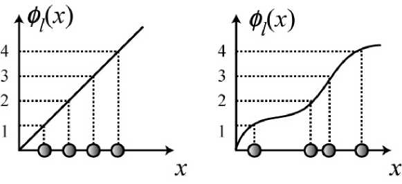
Figure 2: Some examples of the labelling field $\phi_{l}(x)$. If the particles form a perfect lattice of lattice spacing $d$, then $\phi_{l}^{0}(x)=2\pi x/d$, and is just a straight line. Different functions $\phi_{l}(x)$ allow to put the particles at any position in space. Note that $\phi(x)$ is always an increasing function regardless of the position of the particles.

Using this labelling field and the rules for transforming $\delta$ functions

$$\delta(f(x))=\sum_{\mbox{zeros of $f$}}\frac{1}{|f^{\prime}(x_{i})|}\delta(x-x_{i})$$ (18)

one can rewrite the density as

$$\rho(x) = \sum_{i}\delta(x-x_{i})$$ (19)

$$= \sum_{n}|\nabla\phi_{l}(x)|\delta(\phi_{l}(x)-2\pi n)$$

It is easy to see from Fig. 2 that $\phi_{l}(x)$ can always be taken as an increasing function of $x$, which allows to drop the absolute value in (19). Using the Poisson summation formula this can be rewritten

$$\rho(x)=\frac{\nabla\phi_{l}(x)}{2\pi}\sum_{p}e^{ip\phi_{l}(x)}$$ (20)

where $p$ is an integer. It is convenient to define a field $\phi$ relative to the perfect crystalline solution and to introduce

$$\phi_{l}(x)=2\pi\rho_{0}x-2\phi(x)$$ (21)

The density becomes

$$\rho(x)=\left[\rho_{0}-\frac{1}{\pi}\nabla\phi(x)\right]\sum_{p}e^{i2p(\pi\rho_{0}x-\phi(x))}$$ (22)

Since the density operators at two different sites commute it is normal to expect that the field $\phi(x)$ commutes with itself. Note that if one averages the density over distances large compared to the interparticle distance $d$ all oscillating terms in (22) vanish. Thus, only $p=0$ remains and this smeared density is

$$\rho_{q\sim 0}(x)\simeq\rho_{0}-\frac{1}{\pi}\nabla\phi(x)$$ (23)

We can now write the single-particle creation operator $\psi^{\dagger}(x)$. Such an operator can always be written as

$$\psi^{\dagger}(x)=[\rho(x)]^{1/2}e^{-i\theta(x)}$$ (24)

where $\theta(x)$ is some operator. In the case where one would have Bose condensation, $\theta$ would just be the superfluid phase of the system. The commutation relations between the $\psi$ impose some commutation relations between the density operators and the $\theta(x)$. For bosons, the condition is

$$[\psi^{\vphantom{\dagger}}_{B}(x),\psi_{B}^{\dagger}(x^{\prime})]=\delta(x-x^{\prime})$$ (25)

Using (24) the commutator gives

$$e^{+i\theta(x)}[\rho(x)]^{1/2}[\rho(x^{\prime})]^{1/2}e^{-i\theta(x^{\prime})}-[\rho(x^{\prime})]^{1/2}e^{-i\theta(x^{\prime})}e^{+i\theta(x)}[\rho(x)]^{1/2}$$ (26)

If we assume quite reasonably that the field $\theta$ commutes with itself ($[\theta(x),\theta(x^{\prime})]=0$), the commutator (26) is obviously zero for $x\neq x^{\prime}$ if (for $x\neq x^{\prime}$)

$$[[\rho(x)]^{1/2},e^{-i\theta(x^{\prime})}]=0$$ (27)

A sufficient condition to satisfy (25) would thus be

$$[\rho(x),e^{-i\theta(x^{\prime})}]=\delta(x-x^{\prime})e^{-i\theta(x^{\prime})}$$ (28)

It is easy to check that if the density were only the smeared density (23) then (28) is obviously satisfied if

$$[\frac{1}{\pi}\nabla\phi(x),\theta(x^{\prime})]=-i\delta(x-x^{\prime})$$ (29)

One can show that this is indeed the correct condition to use Giamarchi (2004a). Equation (29) proves that $\theta$ and $\frac{1}{\pi}\nabla\phi$ are canonically conjugate. Note that for the moment this results from totally general considerations and does not rest on a given microscopic model. Such commutation relations are also physically very reasonable since they encode the well known duality relation between the superfluid phase and the total number of particles. Integrating by part (29) shows that

$$\pi\Pi(x)=\hbar\nabla\theta(x)$$ (30)

where $\Pi(x)$ is the canonically conjugate momentum to $\phi(x)$.

To obtain the single-particle operator one can substitute (22) into (24). Since the square root of a delta function is also a delta function up to a normalization factor the square root of $\rho$ is identical to $\rho$ up to a normalization factor that depends on the ultraviolet structure of the theory. Thus,

$$\psi^{\dagger}_{B}(x)=[\rho_{0}-\frac{1}{\pi}\nabla\phi(x)]^{1/2}\sum_{p}e^{i2p(\pi\rho_{0}x-\phi(x))}e^{-i\theta(x)}$$ (31)

where the index $B$ emphasizes that this is the representation of a bosonic creation operator. A similar formula can be derived for fermionic operators Giamarchi (2004a). The above formulas are a way to represent the excitations of the system directly in terms of variables defined in the continuum limit, and (31) and (22) are the basis of the bosonization dictionary.

The fact that all operators are now expressed in terms of variables describing collective excitations is at the heart of the use of such representation, since as already pointed out, in one dimension excitations are necessarily collective as soon as interactions are present. In addition the fields $\phi$ and $\theta$ have a very simple physical interpretation. If one forgets their canonical commutation relations, order in $\theta$ indicates that the system has a coherent phase as indicated by (31), which is the signature of superfluidity. On the other hand order in $\phi$ means that the density is a perfectly periodic pattern as can be seen from (22). This means that the system of bosons has “crystallized”. As we now see, the simplicity of this representation in fact allows to solve an interacting system of bosons in one dimension.

3.2 Physical results and Luttinger liquid

What is the Hamiltonian of the system? Using (31), the kinetic energy becomes

$$H_{K}\simeq\int dx\frac{\hbar^{2}\rho_{0}}{2m}(\nabla e^{i\theta})(\nabla e^{-i\theta})=\int dx\frac{\hbar^{2}\rho_{0}}{2m}(\nabla\theta)^{2}$$ (32)

which is the part coming from the single-particle operator containing less powers of $\nabla\phi$ and thus the most relevant. Using (4) and (22), the interaction term becomes

$$H_{\rm int}=\int dxV_{0}\frac{1}{2\pi^{2}}(\nabla\phi)^{2}$$ (33)

plus higher order operators. Keeping only the above lowest order shows that the Hamiltonian of the interacting bosonic system can be rewritten as

$$H=\frac{\hbar}{2\pi}\int dx[\frac{uK}{\hbar^{2}}(\pi\Pi(x))^{2}+\frac{u}{K}(\nabla\phi(x))^{2}]$$ (34)

where I have put back the $\hbar$ for completeness. This leads to the action

$$S/\hbar=\frac{1}{2\pi K}\int dx\;d\tau[\frac{1}{u}(\partial_{\tau}\phi)^{2}+u(\partial_{x}\phi(x))^{2}]$$ (35)

This hamiltonian is a standard sound wave one. The fluctuation of the phase $\phi$ represent the “phonon” modes of the density wave as given by (22). One immediately sees that this action leads to a dispersion relation, $\omega^{2}=u^{2}k^{2}$, i.e. to a linear spectrum. $u$ is the velocity of the excitations. $K$ is a dimensionless parameter whose role will be apparent below. The parameters $u$ and $K$ are used to parameterize the two coefficients in front of the two operators. In the above expressions they are given by

$$\begin{split}uK&=\frac{\pi\hbar\rho_{0}}{m}\\ \frac{u}{K}&=\frac{V_{0}}{\hbar\pi}\end{split}$$ (36)

This shows that for weak interactions $u\propto(\rho_{0}V_{0})^{1/2}$ while $K\propto(\rho_{0}/V_{0})^{1/2}$. In establishing the above expressions we have thrown away the higher order operators, that are less relevant. The important point is that these higher order terms will not change the form of the Hamiltonian (like making cross terms between $\phi$ and $\theta$ appears etc.) but only renormalize the coefficients $u$ and $K$ (for more details see Giamarchi (2004a)). For galilean invariant system the first relation is exactly satisfied regardless of the strength of the interaction Haldane (1981a); Cazalilla (2004a); Giamarchi (2004a).

The low-energy properties of interacting bosons are thus described by an Hamiltonian of the form (34) provided the proper $u$ and $K$ are used. These two coefficients totally characterize the low-energy properties of massless one-dimensional systems. The bosonic representation and Hamiltonian (34) play the same role for one-dimensional systems than the Fermi liquid theory plays for higher-dimensional systems. It is an effective low-energy theory that is the fixed point of any massless phase, regardless of the precise form of the microscopic Hamiltonian. This theory, which is known as Luttinger liquid theory Haldane (1981b, a), depends only on the two parameters $u$ and $K$. Provided that the correct value of these parameters are used, all asymptotic properties of the correlation functions of the system then can be obtained exactly using (22) and (24).

In the absence of a good perturbation theory (e.g. in the interaction) such as (36), it is difficult to compute these coefficients. One has two ways of proceeding. Either one is attached to a particular microscopic model (such as the Bose-Hubbard model for example). In which case the Luttinger liquid coefficients $u$ and $K$ are functions of the microscopic parameters. One thus just needs two relations involving these coefficients that can be computed with the microscopic model and determine these coefficients, thus allowing to compute all correlation functions. How to do that depends on taste and integrability or not of the model. If the model is integrable by Bethe-ansatz such as the Lieb-Liniger model one computes thermodynamics from BA and obtains $u$ and $K$ that way Haldane (1981a); Cazalilla (2004a). If the model is not exactly solvable one can still use numerics such as exact diagonalization, monte-carlo or DMRG technique to compute these coefficients. Because they can be extracted from thermodynamic quantities, their determination suffers usually from very little finite size effects compared to a direct calculation of the correlation functions. The Luttinger liquid theory thus provides, coupled with the numerics, an incredibly accurate way to compute correlations and physical properties of a system. For more details on the various procedures and models see Giamarchi (2004a).

But, of course, a much more important use of Luttinger liquid theory is to justify the use of the boson Hamiltonian and fermion–boson relations as starting points for any microscopic model. The Luttinger parameters then become some effective parameters. They can be taken as input, based on general rules (e.g. for bosons $K=\infty$ for non interacting bosons and $K$ decreases as the repulsion increases, for other general rules see Giamarchi (2004a)), without any reference to a particular microscopic model. This removes part of the caricatural aspects of any modelization of a true experimental system. This use of the Luttinger liquid is reminiscent of the one made of Fermi liquid theory. Very often calculations are performed in solids starting from ‘free’ electrons and adding important perturbations (such as the BCS attractive interaction to obtain superconductivity). The justification of such a procedure is rooted in the Fermi liquid theory, where one does not deal with ‘real’ electrons but with the quasiparticles, which are intrinsically fermionic in nature. The mass $m$ and the Fermi velocity $v_{F}$ are then some parameters. The calculations in $d=1$ proceed in the same spirit with the Luttinger liquid replacing the Fermi liquid. The Luttinger liquid theory is thus an invaluable tool to tackle the effect of perturbations on an interacting one-dimensional electron gas (such as the effect of lattice, impurities, coupling between chains, etc.). I will illustrate such use in the following sections, taking as examples the effects of a periodic potential and a disordered one.

Let us now examine in details the physical properties of such a Luttinger liquid. For this we need the correlation functions. I briefly show here how to compute them using the standard operator technique. More detailed calculations and functional integral methods are given in Giamarchi (2004a). A building block to compute the various observables is

$$G_{\phi\phi}(x,\tau)=\langle T_{\tau}[\phi(x,\tau)-\phi(0,0)]^{2}\rangle$$ (37)

where $T_{\tau}$ is the standard time ordering operator, and $\tau$ the imaginary time Mahan (1981). We absorb the factor $K$ in the Hamiltonian by rescaling the fields (this preserves the commutation relation)

$$\begin{split}\phi&=\sqrt{K}\tilde{\phi}\\ \theta&=\frac{1}{\sqrt{K}}\tilde{\theta}\end{split}$$ (38)

The fields $\tilde{\phi}$ and $\tilde{\theta}$ can be expressed in terms of bosons operator $[b^{\vphantom{\dagger}}_{q},b^{\dagger}_{q^{\prime}}]=\delta_{q,q^{\prime}}$. This ensures that their canonical commutation relations are satisfied. One has

$$\begin{split}\phi(x)&=-\frac{i\pi}{L}\sum_{p\neq 0}\left(\frac{L|p|}{2\pi}\right)^{1/2}\frac{1}{p}e^{-\alpha|p|/2-ipx}(b^{\dagger}_{p}+b^{\vphantom{\dagger}}_{-p})\\ \theta(x)&=\frac{i\pi}{L}\sum_{p\neq 0}\left(\frac{L|p|}{2\pi}\right)^{1/2}\frac{1}{|p|}e^{-\alpha|p|/2-ipx}(b^{\dagger}_{p}-b^{\vphantom{\dagger}}_{-p})\end{split}$$ (39)

where $L$ is the size of the system and $\alpha$ a short distance cutoff (of the order of the interparticle distance) needed to regularize the theory at short scales. The above expressions are in fact slightly simplified and zero modes should also be incorporated Giamarchi (2004a). This will not affect the remaining of this section and the calculation of the correlation functions.

It is easy to check by a direct substitution of (39) in (34) that Hamiltonian (34) with $K=1$ is simply

$$\tilde{H}=\sum_{p\neq 0}u|p|b^{\dagger}_{p}b^{\vphantom{\dagger}}_{p}$$ (40)

The time dependence of the field can now be easily computed from (40) and (39). This gives

$$\phi(x,\tau)=-\frac{i\pi}{L}\sum_{p\neq 0}\left(\frac{L|p|}{2\pi}\right)^{1/2}\frac{1}{p}e^{-\alpha|p|/2-ipx}(b^{\dagger}_{p}e^{u|p|\tau}+b^{\vphantom{\dagger}}_{-p}e^{-u|p|\tau})$$ (41)

The correlation function (37) thus becomes

$$G_{\phi\phi}(x,\tau) =K\langle T_{\tau}[\tilde{\phi}(x,\tau)-\tilde{\phi}(0,0)]^{2}\rangle_{0}$$

$$=2K[\langle\tilde{\phi}(0,0)\tilde{\phi}(0,0)\rangle_{0}-Y(\tau)\langle\tilde{\phi}(x,\tau)\tilde{\phi}(0,0)\rangle_{0}$$

$$\quad-Y(-\tau)\langle\tilde{\phi}(0,0)\tilde{\phi}(x,\tau)\rangle_{0}]$$ (42)

where $Y$ is the step function. One then plugs (41) in (42). The calculation is thus reduced to the averages of factors such as

$$\langle b^{\dagger}_{p}b^{\vphantom{\dagger}}_{p^{\prime}}\rangle_{0}=\delta_{p,p^{\prime}}f_{B}(\epsilon_{p}=u|p|)$$ (43)

and factors such as $bb^{\dagger}=1-b^{\dagger}b$ that can be easily reduced to the above form. $f_{B}$ is the standard Bose factor. At $T=0$ since $\epsilon_{p}>0$ (remember that $p\neq 0$ for the bosons modes) $f_{B}(\epsilon_{q})=0$. Thus, (42) becomes (taking the standard limit $L\to\infty$)

$$G_{\phi\phi}(x,\tau) = K\int_{0}^{\infty}\frac{dp}{p}e^{-\alpha p}[1-e^{-u|\tau|p}\cos(px)]$$ (44)

$$= \frac{K}{2}\log\left[\frac{x^{2}+(u|\tau|+\alpha)^{2}}{\alpha^{2}}\right]$$

Thus, up to the small cutoff $\alpha$, this is essentially $\log(r)$ where $r$ is the distance in space–time. This invariance by rotation in space–time reflects the Lorentz invariance of the action. One can introduce

$$\begin{split}r&=\sqrt{x^{2}+y_{\alpha}^{2}}\\ y_{\alpha}&=u\tau+\alpha{\rm Sign}(\tau)\end{split}$$ (45)

The same calculation with $\theta$ instead of $\phi$ gives exactly the same result with $1/K$ instead of $K$. One can either do it directly or notice that the Hamiltonian is invariant by $\phi\to\theta$ and $K\to 1/K$. The above calculations have been performed at zero temperature. It is easy to obtain the correlation at finite temperature using the same methods. It can also be derived using the conformal invariance of the theory. Such conformal invariance can also be nicely used to obtain the correlations for systems of finite size Cazalilla (2002, 2004a). Other correlations and further details can be found in Giamarchi (2004a).

In order to compute physical observable we need to get correlations of exponentials of the fields $\phi$ and $\theta$. To do so one simply uses that for an operator $A$ that is linear in terms of boson fields and a quadratic Hamiltonian one has

$$\langle T_{\tau}e^{A}\rangle=e^{\frac{1}{2}\langle T_{\tau}A^{2}\rangle}$$ (46)

Thus, for example

$$\langle T_{\tau}e^{i2\phi(x,\tau)}e^{-i2\phi(0,0)}\rangle = e^{-2\langle T_{\tau}[\phi(x,\tau)-\phi(0,0)]^{2}\rangle}$$ (47)

$$= e^{-2G_{\phi\phi}(x,\tau)}$$

If we want to compute the fluctuations of the density

$$\langle T_{\tau}\rho(x,\tau)\rho(0)\rangle$$ (48)

we obtain, using (22)

$$\langle T_{\tau}\rho(x,\tau)\rho(0)\rangle=\rho_{0}^{2}+\frac{K}{2\pi^{2}}\frac{y_{\alpha}^{2}-x^{2}}{(x^{2}+y_{\alpha}^{2})^{2}}+\rho_{0}^{2}A_{2}\cos(2\pi\rho_{0}x)\left(\frac{\alpha}{r}\right)^{2K}\\ +\rho_{0}^{2}A_{4}\;\cos(4\pi\rho_{0}x)\left(\frac{\alpha}{r}\right)^{8K}+\cdots$$ (49)

Here, the lowest distance in the theory is $\alpha\sim\rho_{0}^{-1}$. The amplitudes $A_{i}$ are non-universal objects. They depend on the precise microscopic model, and even on the parameters of the model. Contrary to the amplitudes $A_{n}$, which depend on the precise microscopic model, the power-law decay of the various terms are universal. They all depend on the unique Luttinger coefficient $K$. Physically the interpretation of the above formula is that the density of particles has fluctuations that can be sorted compared to the average distance between particles $\alpha\sim d=\rho_{0}^{-1}$. This is shown on Fig. 3.

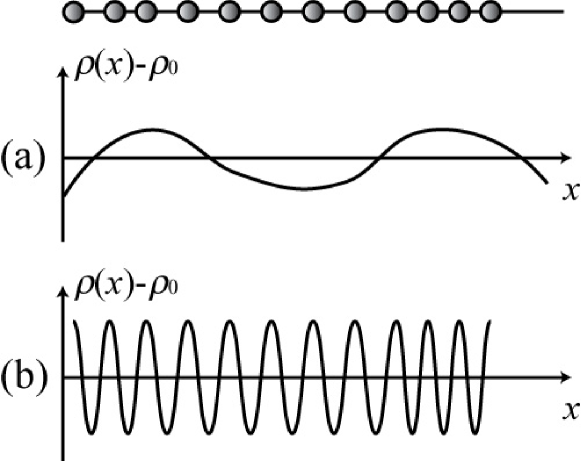
Figure 3: The density $\rho(x)$ can be decomposed in components varying with different Fourier wavevectors. The characteristic scale to separate these modes is the inter particle distance. Only the two lowest harmonics are represented here. Although they have very different spatial variations both these modes depends on the same smooth field $\phi(x)$. (a) the smooth variations of the density at lengthscale larger than the lattice spacing. These are simply $-\nabla\phi(x)/\pi$. (b) The density wave corresponding to oscillations of the density at a wavevector $Q=2\pi\rho_{0}$. These modes correspond to the operator $e^{i\pm 2\phi(x)}$.

The fluctuations of long wavelength decay with a universal power law. These fluctuations correspond to the hydrodynamic modes of the interacting boson fluid. The fact that their fluctuation decay very slowly is the signature that there are massless modes present. This corresponds to the sound waves of density described by (34). However the density of particles has also higher fourier harmonics. The corresponding fluctuations also decay very slowly but this time with a non-universal exponent that is controlled by the LL parameter $K$. This is also the signature of the presence of a continuum of gapless modes, that exists for Fourier components around $Q=2n\pi\rho_{0}$ as shown in Fig. 3. In the Tonks-Girardeau limit, this mode is simply the low energy mode corresponding to transferring one fermion from one side of the Fermi surface to the other, leading to a $2k_{F}$ momentum transfer. In higher dimensions and with a true condensate such a gapless mode would not exist, and only the modes close to $q\sim 0$ would remain (the Goldstone modes corresponding to the phase fluctuations). The other gapless mode is thus the equivalent of the roton minimum that only exists at a finite energy in high dimensions but would be pushed to zero energy in a one dimensional situation Nozieres (2004); Iucci et al. (2006); Cazalilla et al. (2006). As we discussed the coefficient $K$ goes to infinity when the interaction goes to zero which means that the correlations in the density decays increasingly faster with smaller interactions. This is consistent with the idea that the system becoming more and more superfluid smears more and more its density fluctuations.

Let us now turn to the single particle correlation function

$$G(x,\tau)=\langle T_{\tau}\psi(x,\tau)\psi^{\dagger}(0,0)\rangle$$ (50)

At equal time this correlation function is a direct measure on whether a true condensate exists in the system. Its Fourier transform is the occupation factor $n(k)$. In presence of a true condensate, this correlation function tends to $G(x\to\infty,\tau=0)\to|\psi_{0}|^{2}$ the square of the order parameter $\psi_{0}=\langle\psi(x,\tau)\rangle$ when there is superfluidity. Its Fourier transform is a delta function at $q=0$, as shown in Fig. 4. In one dimension, no condensate can exist since it is impossible to break a continuous symmetry even at zero temperature, so this correlation must always go to zero for large space or time separation. Using (31) the correlation function can easily be computed. Keeping only the most relevant term ($p=0$) leads to (I have also put back the density result for comparison)

$$\begin{split}\langle T_{\tau}\psi(r)\psi^{\dagger}(0)\rangle&=A_{1}\left(\frac{\alpha}{r}\right)^{\frac{1}{2K}}+\cdots\\ \langle T_{\tau}\rho(r)\rho(0)\rangle&=\rho_{0}^{2}+\frac{K}{2\pi^{2}}\frac{y_{\alpha}^{2}-x^{2}}{(y_{\alpha}^{2}+x^{2})^{2}}+A_{3}\cos(2\pi\rho_{0}x)\left(\frac{1}{r}\right)^{2K}+\cdots\end{split}$$ (51)

where the $A_{i}$ are the non-universal amplitudes. For the non-interacting system $K=\infty$ and we recover that the system possesses off-diagonal long-range order since the single-particle Green’s function does not decay with distance. The system has condensed in the $q=0$ state. As the repulsion increases ($K$ decreases), the correlation function decays faster and the system has less and less tendency towards superconductivity. The occupation factor $n(k)$ has thus no delta function divergence but a power law one, as shown in Fig. 4.

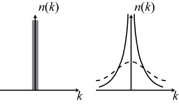
Figure 4: Momentum distribution $n(k)$ for the bosons as a function of the momentum $k$. (left) For non-interacting bosons all bosons are in $k=0$ state, thus $n(k)\propto\delta(k)$ (thick line). (right) As soon as interactions are introduced a true condensate cannot exist. The $\delta$ function is replaced by a power law divergence with an exponent $\nu=1-1/(2K)$ (solid line). In a Mott insulating phase or a Bose glass phase, the superfluid correlation functions decay exponentially leading to a rounding of the divergence and a lorentzian like shape for $n(k)$. This is indicated by the dashed line.

Note that the presence of the condensate or not is not directly linked to the question of superfluidity. The fact that the system is a Luttinger liquid with a finite velocity $u$, implies that in one dimension an interacting boson system has always a linear spectrum $\omega=uk$, contrary to a free boson system where $\omega\propto k^{2}$. Such a system is thus a true superfluid at $T=0$ since superfluidity is the consequence of the linear spectrum Mikeska and Schmidt (1970). Note that of course when the interaction tends to zero $u\to 0$ as it should to give back the quadratic dispersion of free bosons.

An even better criterion for the occurrence of superfluidity or other ordered phases is provided by the susceptibilities. They are the Fourier transforms of the correlation functions

$$\chi(\omega_{n},k)=\int dxd\tau\chi(x,\tau)$$ (52)

It is easy to see by simple dimensional analysis that if the correlation decays as a powerlaw $\chi(r)\sim(1/r)^{\mu}$ then the susceptibility behaves as $\max(\omega,k,T)^{\mu-2}$. The susceptibilities give direct indications on the phase that the system would tend to realize, if many chains were put together and coupled by a mean-field interaction. An RPA calculation would then directly lead to the stabilization of three dimensional order, stabilizing the phase with the most divergent susceptibility. From (51) the charge and superfluid susceptibilities diverge as

$$\begin{split}\chi_{\rho}&=T^{2-2K}\\ \chi_{\psi}&=T^{2-\frac{1}{2K}}\end{split}$$ (53)

This leads thus to the “phase diagram” of Fig. 5.

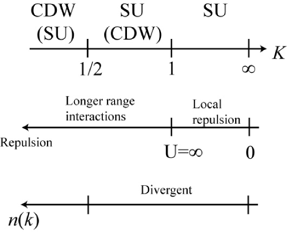
Figure 5: “Phase diagram” for (incommensurate) one-dimensional bosons, as a function of the parameter $K$. The phase indicated corresponds to the most divergent susceptibility, while a phase in parenthesis corresponds to a subdominant divergence. The value $K=1$ corresponds to the Tonks-Girardeau limit where the bosons are hard core and behave very similarly to spinless fermions. The region where $n(k)$ has a singularity at $k=0$ is indicated on the bottom graph.

Let me again emphasize that there is no true long range order in the system but only algebraically decaying correlations. Such a phase diagram indicates the dominant tendency of the system. Note also that the superfluid susceptibility is not identical to $n(k)$, since this one only contains the correlation at equal time. Its divergence is different and, as shown in Fig. 4 is given by

$$n(k)\propto k^{\frac{1}{2K}-1}$$ (54)

As we already discussed, for a purely local interaction, when the repulsion becomes infinite the system becomes equivalent to free spinless fermions. Indeed two particles cannot be on the same site and the particles are totally free except for this constraint. In that case the decay of the density (51) should be the one of free fermions, i.e. $1/r^{2}$. This can be realized if $K=1$. Note that the Green function of the bosons does not become the correlation function of spinless fermions since they still represent different statistics. In particular the boson correlation function still diverges at $k=0$ even in the TG limit. In that limit since $K=1$ the $n(k)$ has a square root divergence. For a purely local repulsion, $K=1$ is the minimal value that $K$ can reach. Of course, longer range repulsion between bosons can make the system reach smaller values of $K$. More details and mapping on other systems (classical and quantum such as spin chains) can be found in Giamarchi (2004a). Testing these predictions in cold atomic systems is complicated by the presence of the harmonic trap Stöferle et al. (2004); Kinoshita et al. (2004); Paredes et al. (2004); Cazalilla (2004b)

4 Mott transition

4.1 Basic Ideas

Let us now investigate the effects of a lattice on such a bosonic system Haldane (1981a); Fisher et al. (1989); Scalettar et al. (1991); Giamarchi (1992, 1997); Büchler et al. (2003). For noninteracting bosons the lattice just provides a renormalization of the kinetic energy as shown in (14). When interactions are present, a lattice leads to a radically new physics. In particular when the density of carriers is commensurate with the lattice, another interaction induced phenomenon occurs. In that case the system can become an insulator. This is the mechanism known as Mott transition Mott (1949, 1990), and is a metal-insulator transition induced by the interactions. The physics of a Mott insulator is well-known and illustrated in Fig. 6.

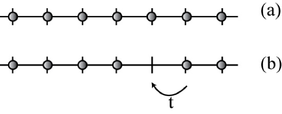
Figure 6: (a) If there is one particle per lattice site and the repulsion among particles is strong, a plane wave state for the particles is energetically unfavorable since the density is uniform. It is better to localize the particles on each site. Such a state is a Mott insulator since hopping would cost an energy of the order of the interaction $U$ among particles. (b) If the system is doped the extra particles or holes can propagate without any energy cost from the interactions and gain some kinetic energy  $\sim\!t$. The system is then in general superfluid again.

If the repulsion $U$ among the particles is much larger than the kinetic energy $t$, then the plane wave state is not very favorable since it leads to a uniform density where particles experience the maximum repulsion. It is more favorable to localize the particles on the lattice sites to minimize the repulsion and the system is an insulator for one particle per site. If the system is weakly doped compared to a state with one particle per site the holes can propagate without experiencing repulsion, the system is thus in general a superfluid again but with a number of carriers proportional to the doping. The above argument shows that, in high dimensions, one usually needs a finite (and in general of the order of the kinetic energy) repulsion to reach that state. For further details on the Mott transition in higher dimension see Georges et al. (1996); Imada et al. (1998). It is important to note that one particle per site is not the only commensurate filling where one can in principle get a Mott insulator, but that every commensurate filling can work, in principle, depending on the interactions. This is illustrated in Fig. 7.

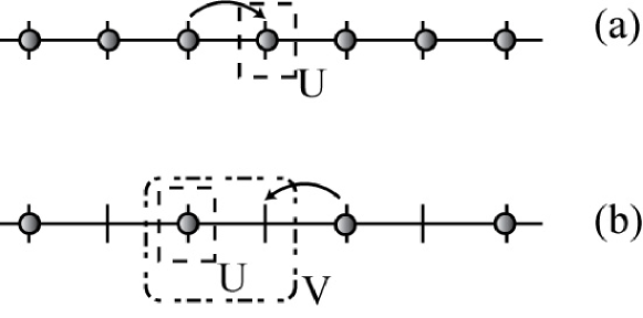
Figure 7: (a) In a model with onsite interactions ($U$) a Mott insulator only exists for one particle per site. (b) Nearest neighbor interactions $V$ can stabilize the insulating state for up to one particle every two sites. And so on with longer ranger interactions. The longer the range of the interaction, the higher the commensurability for which one can have a Mott insulator provided the interactions are large enough.

It is indeed easy to see that for large enough onsite ($U$) and nearest neighbor ($V$) repulsion a quarter-filled system is an ordered Mott insulator. As I will discuss in more details below, and as is clear from Fig. 7, in order to stabilize a structure with a certain spacing between the particles one needs interactions that can reach at least to such a distance. In particular for cold atoms, since the interactions are mostly local, one can expect a Mott insulator to be possible for one (or any integer) number of fermions per site. Other insulating phases (1 boson each two sites etc.) would need longer range interactions.

To study the Mott transition, we thus consider the application of a periodic potential of period wavevector $Q=2\pi/a$. This can be realized by taking

$$V_{L}(x)=\sum_{n}V^{0}_{n}\cos(Qnx)$$ (55)

In fact in cold atomic gases it is easy to realize systems with only one harmonic as was shown in (10). In that case $n=1$ is the only existing Fourier component. In the lattice potential is very large, then as we already discussed the kinetic energy gets very small and one has a rather trivial insulating case. In the Bose-Hubbard language this corresponds to the limit $U\gg t$. The particles are nearly “classically” localized. The case where either the lattice or the interactions are small is much more subtle.

4.2 Bosonization solution

Using (55) and the expression (22) for the density, we see that terms such as

$$\int dxe^{i(Qn-2p\pi\rho_{0})x}e^{-i2p\phi(x)}$$ (56)

appear. Because the field $\phi(x)$ is a smooth field varying slowly at the scale of the interparticle distance, if oscillating terms remain in the integral they will average out leading to a negligible contribution. The corresponding operator would then disappear from the Hamiltonian. In order for such terms to be relevant, one needs to have no oscillating terms in (56). This occurs if

$$nQ=2\pi\rho_{0}p$$ (57)

If we use $\rho_{0}=1/d$ where $d$ is the distance between particles one has

$$nd=pa$$ (58)

The corresponding term contributing to the Hamiltonian is

$$H_{L}\propto V^{0}_{n}\int dx\;\cos(2p\phi(x))$$ (59)

The periodic potential has thus changed for commensurate fillings the simple quadratic hamiltonian (34) of the Luttinger liquid into a sine-Gordon Hamiltonian (34) plus (59). This sine-Gordon Hamiltonian describes in fact in one dimension the physics of any Mott transition Giamarchi (2004a).

Although the term (59) has been derived here for a weak potential, it appears also in the opposite limit of a strong barrier if the filling is commensurate, showing that the two limits are in fact smoothly connected. Indeed if one starts from the Bose-Hubbard model, the lattice potential $V_{L}$ is not present anymore, but the position of the particles is quantized $x_{j}=ja$ where $j$ is an integer. It means that when one writes the interaction term one should pay special attention to this when going to the continuum limit. The fields $\phi$ are smooth so for them one has $\phi(x_{j})\to\phi(x)$ and one can take for them the continuum limit. This is not the case for the oscillating factors in (22). Such terms are of the form $e^{2p\pi\rho_{0}x_{j}}$. Since $\rho_{0}=1/a$ they oscillate fast and replacing $x_{j}\to$ is impossible in such terms. If one was simply doing it, the fact that the oscillating factors should vanish in order to avoid the integral over $x$ to be killed would impose for the interaction term

$$U\sum_{j}n_{j}(n_{j}-1)\to U\rho_{0}^{2}a\int dx\sum_{p,p^{\prime}}e^{i(p+p^{\prime})2\pi\rho_{0}x}e^{-i2(p+p^{\prime})\phi(x)}$$ (60)

to choose opposite $p=-p^{\prime}$ in (22) for each of the densities. This is the normal interaction, that conserves the total momentum of the particles. However due to the discreteness of $x_{j}$ other terms are possible. Let us choose for one density $p=0$ ($n_{j}\to\rho_{0}$) and for the other one keep the term with $p$. Then the interaction term becomes

$$Ua^{2}\rho_{0}^{2}\sum_{j}e^{2p\pi\rho_{0}x_{j}}e^{-i2p\phi(x_{j})}\to Ua^{2}\rho_{0}^{2}\sum_{j}e^{2p\pi\rho_{0}x_{j}}e^{-i2p\phi(x)}$$ (61)

Now normally such terms would be killed by the oscillating factor, but if $2p\pi\rho_{0}a=2\pi n$ then the exponential term is always one, and the corresponding interaction remains in the continuum limit

$$U\rho_{0}^{2}a\int dxe^{-i2p\phi(x)}$$ (62)

which is exactly the same condition and operator than the ones leading to (59). On a physical basis, these interactions, known as the umklapp process Dzyaloshinskii and Larkin (1972), do not conserve the momentum. However on a lattice momentum needs only to be conserved modulo one vector of the reciprocal lattice, the extra momentum being transferred as a whole to the periodic structure. Note that the main difference between the weak and strong lattices is the strength of this umklapp process. For the weak lattice (59) the strength of the umklapp is simply the amplitude of the periodic potential. For very large lattice, the umklapp strength becomes now proportional to the interaction $U$. Of course such a representation works if the interaction remains reasonably weak compared to the kinetic energy $t$, otherwise the amplitudes of the operators cannot be determined directly as discussed above.

Doping causes a slight deviation from the condition (58). This can be seen in two ways. The simplest is to use the fact that the density is slightly different than the commensurate density that leads to the relation (59). Part of the oscillating term remain, but if the deviation is quite small these oscillations will only be important at very large lengthscales. One should thus keep the corresponding term. In that case the umklapp term (61) becomes

$$H_{u}=g_{u}\int dx\;\cos(2p\phi(x)-\delta x)$$ (63)

where $p$ is the order of the commensurability and $\delta$ is the doping, i.e. the deviation of the density from the commensurate value. Another way to recover this result is to start from the commensurate case and apply a chemical potential. Using the boson representation (22) the chemical potential term becomes

$$\mu_{0}\int dx\frac{1}{\pi}\nabla\phi(x)$$ (64)

The chemical potential can be absorbed by a redefinition of the field $\phi$. Introducing

$$\begin{split}\tilde{\phi}(x)&=\phi(x)+\frac{K}{u}\mu_{0}x\\ \tilde{\theta}(x)&=\theta(x)\end{split}$$ (65)

the Hamiltonian is now quadratic again in $\tilde{\phi}$ while the commensurate umklapp (58) is now changed into (63). We see again that an incommensurate filling is washing out the cosine, therefore leading back to a Luttinger liquid state. However if the deviations from commensurability are small the doping is only acting for lengthscales larger than $1/\delta$ that can be quite large compared to the lattice spacing. This leads to an interesting physics that I examine below. For more details on the Mott transition and the difference between working with a fixed density and a fixed chemical potential see Giamarchi (2004a). The Hamiltonian (63) thus provides a complete description of the Mott transition and the Mott insulating state in one dimension. To change the physical properties of a commensurate system one has thus two control parameters. One can vary the strength of the interactions while staying at commensurate filling, or vary the chemical potential (or filling) while keeping the interactions constant. One can thus expect two different classes of transition to occur.

Let us first deal with the transition where the filling is kept commensurate and interaction strength is varied (Mott-U transition). In that case $\delta=0$ and (63) is just a sine-Gordon Hamiltonian. As is well known this Hamiltonian has a quantum phase transition at $T=0$ as a function of the Luttinger parameter $K$, and thus as a function of the strength (and range) of the interactions. This transition is a Berezinskii–Kosterlitz–Thouless (BKT) transition Kosterlitz (1974). I will not explain here how to analyze such a transition, but simply remind how one can get renormalization equations giving the phase diagram. The idea is to vary the cutoff $\alpha$ of the theory to eliminate short distance degrees of freedom, and capture the large distance physics. Parametrizing the cutoff as $\alpha(l)=\alpha e^{l}$ one can establish how the parameters in the Hamiltonian must vary when $l$ is varied in order to keep the long distance physics invariant. The renormalization equations for $K$ and the strength of the umklapp term (59) are

$$\begin{split}\frac{dK}{dl}&=-\frac{p^{2}K^{2}}{8\pi\alpha^{2}u}(V^{0}_{n})^{2}\\ \frac{dV^{0}_{n}}{dl}&=(2-p^{2}K)V^{0}_{n}\end{split}$$ (66)

The second equation can be understood by looking at the scaling dimension of the second order perturbation theory in (59). Such a term behaves as

$$(V^{0}_{n})^{2}\int dxd\tau\int dx^{\prime}d\tau^{\prime}\langle T_{\tau}e^{i2p\phi(x,\tau)}e^{-i2p\phi(x,\tau)}\rangle$$ (67)

Using the fact that the correlation decay as a power law with an exponent $2p^{2}K$ the scaling dimension of this integral is $L^{4-2p^{2}K}$. Such dimension leads directly to the second equation in (66). The first equation is more subtle to obtain Giamarchi (2004a). Clearly these equations define two regions of parameters. If $K$ is large, $V^{0}_{n}$ decrease when $l$ increases which means that the periodic potential is less and less important. On the contrary, if $K$ is small, $V^{0}_{n}$ increases and the cosine terms is more and more relevant in the Hamiltonian. The critical value is $K_{c}=2/p^{2}$ where $p$ is the order of the commensurability. For larger values of $K$ the cosine is irrelevant and the system is massless. For $K<K_{c}$ the cosine is relevant and the system is massive. This opening of a gap corresponds to the Mott transition and the system becomes an insulator. The larger the commensurability the smaller $K$ needs to be for the system to become insulating. From (58) we see that for the bosons $p=1$ corresponds to a commensurability of one (or 2, 3, …, which would correspond to higher $n$) boson per site ($n=1$). This is shown in Fig. 8.

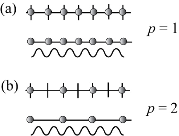
Figure 8: Commensurabilities for the boson system. (Bottom) Bosons in the continuum. The lattice is reintroduced as a periodic potential. (Top) The bosons are defined directly on a lattice. The two descriptions lead to the same physics. (a) A commensurability of one boson per site. For the periodic potential it means that the density modulation has the same period than the external periodic potential. This is the only insulating phase that can be stabilized with local interactions. (b) A commensurability of one boson every two sites. In that case the period of the density modulation is twice the one of the external potential.

In that case the critical value is $K_{c}=2$, which corresponds to strong but finite repulsion. This means that, contrarily to the higher dimensional case above a certain threshold of interactions even a arbitrary weak lattice will lead to a Mott insulator. This is a very surprising result, and quite different from our intuition or the behavior in higher dimension where one only gets a Mott insulator when the kinetic energy is small. For one boson each two sites one has $p=2$ as shown in Fig. 8. The critical value is $K_{c}=1/2$. As discussed this cannot be reached for a local interactions, but nearest neighbor repulsion allows to reach this value and to get a Mott phase. Since for local interactions $1\leq K<\infty$, one recovers, directly from the Luttinger theory the argument that one cannot obtain an ordered phase with a separation of the particles larger than the range of the interaction. The critical properties of the transitions are the ones of the BKT transition: $K$ jumps discontinuously from the universal value $K_{c}$ at the transition in the superfluid (non-gapped) regime to zero in the Mott phase (since there is a gap). Since the velocity is not renormalized it means using that the compressibility goes to a constant at the transition and then drops discontinuously to zero inside the Mott phase. A summary of the critical properties of the Mott transition is given in Fig. 9.

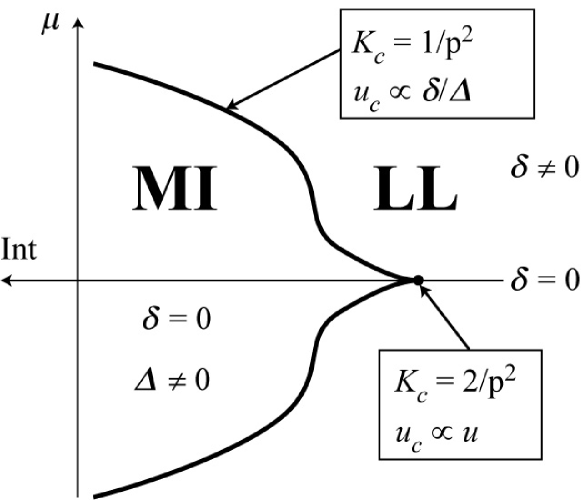
Figure 9: Phase diagram close to a commensurability of order $p$ ($p=1$ for one boson per site and $p=2$ for one boson every two sites). Int denotes a general (that is, not necessarily local) repulsive interaction. $\mu$ is the chemical potential, $\delta$ the doping and $\Delta$ the Mott gap. MI and LL are respectively the Mott insulator the Luttinger liquid (massless) phases. The critical exponent $K_{c}$ and velocity $u_{c}$ at the transition depend on whether it is a Mott-$U$ or Mott-$\delta$ transition. (After Giamarchi (1997).)

In the Mott phase the single-particle Green’s function decays exponentially since the field $\theta$ is dual to the field $\phi$ which is ordered. The characteristic length of decay is $\xi=u/\Delta$ where $\Delta$ is the Mott gap. At the transition the single-particle Green’s function decays with a universal exponent $1/(2K_{c})$ ($1/4$ for one boson per site, $1$ for one boson every two sites, etc.). Note that in the LL phase the system is a perfect conductor (superfluid). A measure is given by the charge stiffness that is the Drude part of the conductivity $\sigma(\omega)={\mathcal{D}}\delta(\omega)$. A finite charge stiffness means thus a perfect conductor for dc transport. The charge stiffness of the LL is finite ${\mathcal{D}}=u_{c}K_{c}$. It jumps discontinuously to zero at the Mott-$U$ transition. In the Mott phase, the system is incompressible. For more details see Giamarchi (2004a).

Let me briefly comment on the physics of the doped system (Mott-$\delta$ transition) Giamarchi (1991). As can be seen from (63) the doping destroys the cosine and thus the Mott phase. It is clear that the oscillating term will kill the cosine at a lengthscale of order $1/\delta$. One has the competition between two terms: the cosine that would like to keep $\phi$ as constant as possible and the doping (or the chemical potential) that would like to tilt $\phi$ so that $\phi=K\mu_{0}x/u$ as can be seen from (64). The way this competition takes place is not to give an homogeneous slope to $\phi$, but to keep $\phi$ commensurate (i.e. locked into one of the minima of the cosine) over a region of order $1/\delta$ and then create a soliton connecting two adjacent minima of the cosine. This is shown in Fig. 10. These solitons act in fact like spinless fermions with some interaction between them. This can be seen by mapping the sine-Gordon Hamiltonian (34) plus (63) to a spinless fermion model (known as massive Thiring model Giamarchi (2004a)). The remarkable fact is that close to the Mott-$\delta$ transition the solitons become non-interacting, and one is simply led to a simple semi-conductor picture of two bands separated by a gap (see Fig. 10). The Mott-$\delta$ transition is thus of the commensurate-incommensurate type Japaridze and Nersesyan (1978); Pokrovsky and Talapov (1979); Schulz (1980); Haldane et al. (1983).

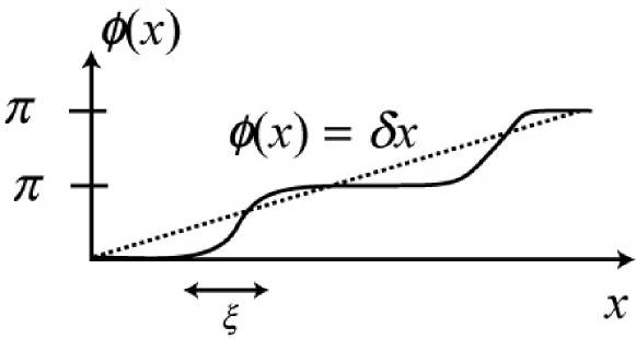
Figure 10: Profile of the field $\phi(x)$ in presence of a commensurate potential and a finite doping $\delta$. In the absence of commensurate potential the doping would impose a slope $\phi(x)=\delta x$ (dashed line). In the presence of the commensurate potential $\cos(2\phi(x))$ it is more favorable energetically to maintain commensurability as much as possible and to proceed from one of the minima of the cosine to the next by making a soliton (full line). The size of such solitons is $\xi\propto u/\Delta$ where $\Delta$ is the Mott gap. These soliton behave for very small doping as spinless fermions.

This image has to be used with caution since the solitons are only non-interacting for infinitesimal doping (or for a very special value of the initial interaction) and has to be supplemented by other techniques Giamarchi (1991). Nevertheless it provides a very appealing description of the excitations and a good guide to understand the phase diagram and transport properties. The transition by varying the chemical potential occurs when the chemical potential equals the charge gap. The density in the incommensurate phase varies as $n\sim(\mu-\mu_{c})^{1/2}$ . The universal (independent of the interactions) value of the exponents $K_{c}^{\delta}=1/p^{2}$ is half of the one of Mott-U transition, as shown in Fig. 9. Since at the Mott-$\delta$ transition the chemical potential is at the bottom of a band the velocity goes to zero with doping. This leads to a continuous vanishing of the charge stiffness ${\mathcal{D}}\sim\delta/\Delta$ where $\delta$ is the doping and $\Delta$ the Mott gap and a divergent compressibility. For more details see Giamarchi (2004a).

4.3 Extensions

As we saw in the previous section, the fact that interactions are able to lead to a Mott insulator phase has several important consequences. We have now a fairly good understanding of the properties of this phase in the pure and homogeneous one dimensional case. There are of course many open questions and active research subjects connected to this problem. There are too numerous to be all mentioned here, so I will simply briefly mention two of them.

First, in cold atomic gases, in addition to the optical lattice there is usually the harmonic confining potential (7). As was already discussed, it acts as a chemical potential. The density is thus non-uniform, and there is thus no meaning as looking at the system as wholly in a commensurate Mott state or not. However as we saw, upon small doping, a Mott insulator prefers to keep the commensurability as much as possible and makes discomensurations between two commensurate regions. In presence of the trap one can thus expect a similar behavior, and to have sequences of incommensurate regions separated by commensurate ones. How these regions are organized is an interesting question, that has been intensely studied Rigol and Muramatsu (2005); Kollath et al. (2004); Wessell et al. (2004); Pedri and Santos (2003); Gangardt (2004). Another important question connected to this problem is how to probe for the existence of such an insulating state. As discussed before measuring the momentum distribution $n(k)$ gives direct information, since it has a divergence at $q=0$ for a superfluid phase and none in the insulating one Greiner et al. (2002); Stöferle et al. (2004); Richard et al. (2003). However, $n(k)$ is only providing limited information, and would also be much less informative in the case of fermion where one has essentially a broadened step at the Fermi energy regardless of whether the system is superconducting or insulating. It is thus important to study other probes of the Mott phase such as noise Altman et al. (2004); Fölling et al. (2005) or shaking of the lattice Stöferle et al. (2004); Schori et al. (2004). Understanding the physics of such shaken lattices is an interesting problem for which I refer the reader to the literature Batrouni et al. (2005); Reischl et al. (2005); Iucci et al. (2006); Kollath et al. (2006).

Another interesting class of problems is to determine how the 1D Mott insulating properties can affect the physics of the system when there is not a single chain but many chains coupled together. More generally it is important to determine how the one-dimensional physics is changed when one goes from a purely one-dimensional system to a two- or three-dimensional situation. Such a crossover between the one dimensional properties and the three dimensional ones is particularly important since many systems are made of coupled one dimensional chains Giamarchi (2004a, b). Cold atomic systems provide a very controlled way to probe for such a physics, since it is possible to control the strength of the optical lattice in each direction.

If the transverse optical lattice is large it can be treated by the same tight binding approximation than the one leading to (12). The most important term describing the coupling between the chains is the interchain tunnelling traducing the fact that single particles are able to hop from one chain to the next

$$H_{\perp}=-\int dx\sum_{\langle\mu,\nu\rangle}t_{\perp,\mu,\nu}[\psi^{\dagger}_{\mu}(x)\psi^{\vphantom{\dagger}}_{\nu}(x)+{\rm h.c.}]$$ (68)

where $\langle\mu,\nu\rangle$ denotes a pair of chains, and $t_{\perp,\mu,\nu}$ is the hopping integral between these two chains. These hopping integrals are of course directly determined by the overlap of the orbitals of the various chains. In addition to the single particle hopping, there are of course also in principle direct interactions terms between the chains. Such terms can be density-density or spin-spin exchange. However they are easy to treat using mean field approximation. For example a spin-spin term $S_{\mu}S_{\nu}$ can be viewed, in a mean field approximation, as an effective ‘classical’ field acting on chain $\nu$: $S_{\mu}S_{\nu}\to\langle S_{\mu}\rangle S_{\nu}$. Thus, at least for an infinite number of chains for which one could expect a mean field approach to be qualitatively correct, the physics of such a term is transparent: it pushes the system to an ordered state. Note that for cold atoms since the interactions are short range such terms do not normally exist and (68) is the only term coupling the chains. For other cases see Giamarchi (2004a).

The single particle hopping is more subtle to treat. For fermions no mean field description is possible since a single fermion operator has no classical limit. It is thus impossible to approximate $\psi^{\dagger}_{\mu}(x)\psi^{\vphantom{\dagger}}_{\nu}(x)$ as $\langle\psi^{\dagger}_{\mu}(x)\rangle\psi^{\vphantom{\dagger}}_{\nu}(x)$, which makes the solution of the problem of coupled chains quite complicated Arrigoni (2000); Georges et al. (2000); Biermann et al. (2001); Cazalilla et al. (2005). For bosons one is in a slightly better situation since the single boson operator has a mean field value. However even in that case there is a direct competition between this interchain hopping that would like to stabilize a three dimensional superfluid phase and the 1D Mott insulating term that would favor an insulating state. As a function of the strength of the interchain hopping there is thus a deconfinement transition where the system goes from a 1D insulator made of essentially uncoupled chains, to a an anisotropic 3D superfluid. Such a transition has been studied both theoretically Ho et al. (2004); Cazalilla et al. (2006) and experimentally Stöferle et al. (2004); Köhl et al. (2004) and i refer the reader to these references for more details. Quite generally such a transition is relevant in various other type of systems as well Giamarchi (2004a, b).

5 Disorder effects: Bose glass

We have examined in the previous section the effects of a periodic potential on an interacting bosonic system. Another important class of potential, leading to radically new physics, is the case of a disordered potential. Here again the bosonization solution is a powerful tool to tackle this problem.

5.1 Disorder in quantum systems

Disorder for quantum problems is a longstanding problem. In condensed matter, some level of disorder is unavoidable, and it is thus necessary to deal with it. The naive expectation is to think that the disorder will have weaker effects for a quantum system than for a classical one. Indeed, as shown in Fig. 11

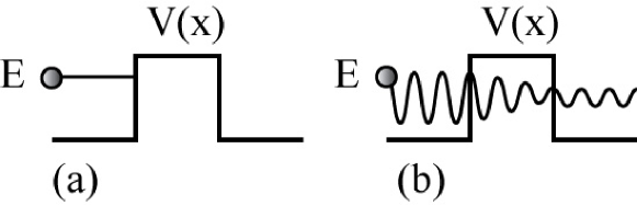
Figure 11: (a) A classical particle of energy $E$ smaller than the disorder $V(x)$ at a given point is totally blocked. (b) A quantum mechanical system of the same energy can pass through the barrier by tunnel effect. One could therefore naively think that quantum systems are much less localized by disorder than their classical equivalents. In fact it is exactly the contrary that happens.

one can imagine that waves in a quantum system have more ease to pass the barriers induced by the disorder since they can use tunnel effect. It was thus a major surprise when Anderson showed Anderson (1958) that it was in fact exactly the opposite effect that occurred for non-interacting quantum particles. Indeed because of the constructive interferences of two paths that are deduced by time inversion there is an additional probability for a particle to be backscattered by the disorder Bergmann (1984). Loosely speaking one should add the wave functions, and thus squaring them getting a factor of four, instead of the naive factor of two of two paths that would not interfere. The main effect is that the wavefunctions of the system, instead of being plane waves, now decay exponentially in space. This phenomenon, known as Anderson localization is strongly dependent on dimension. Simple scaling arguments show that all states should be localized in one and two dimensions Abrahams et al. (1979). In three dimensions, a mobility edge in energy exists below which states are localized and above which they are extended. An important characteristic of such states is thus the localization length $\xi$ characterizing the spatial decay of the localized states. This phenomenon is now well understood for noninteracting particles. For Fermions, i.e. electrons is condensed matter, interactions do exist. However because of the Pauli principle, the important electrons, at the Fermi level have a large kinetic energy $E_{F}$. If this energy is large compared to their interaction it is very reasonable to assume that the noninteracting limit is a good starting point. Indeed, the corresponding predictions for the localization localization have been spectacularly confirmed experimentally Bergmann (1984).

Treating the combined effects of interactions and disorder is a particularly challenging problem, even for fermions. Indeed because of the disorder the motion of the particles becomes much slower than the one of free particles. From ballistic it becomes diffusive at best, which means that two particles can spend more time close to each other. There is thus an extremely strong reinforcement of the interactions by the disorder Altshuler and Aronov (1985); Finkelstein (1984). This leads to singularities and to a physics that is still under debate. Here again the effect of the dimension is crucial, since the singularities increase with lowering dimension. One can expect one dimension, where disorder lead to all state being localized and the interaction leads to the Luttinger liquid state, to be particularly special. I will not dwell further on this problem here and refer the reader to the above literature for further references.

The case of bosons is even more interesting. Indeed in that case the noninteracting case cannot even be used as a reasonable starting point. To understand this let us simply look at a disorder that would take two values $\pm V_{0}$ on each site. Let us assume that one can find a region of space of length $L_{0}$, as shown in Fig. 12. Such a region always exists with a probability $e^{-L_{0}/L_{c}}$ where $L_{c}$ is the characteristic correlation length of the disorder.

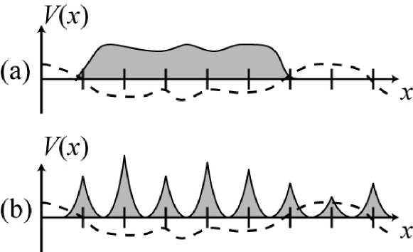
Figure 12: A cartoon of free versus interacting bosons in the presence of disorder (represented by the dashed line). (a) Free boson all condense in a large enough well of the random potential. Since the density is infinite, this situation is unstable when interactions are added. (b) the repulsion prevents the bosons to condense in the same site. Their behavior is thus much closer to fermions, where various minima of the random potential have to be used. Since one can still pile up many bosons in the same minima, the deep minima of the random potential are well smoothed by the bosons.

The lowest energy of one boson confined to this region can be readily computed. Because the boson is confined to a region of size $L_{0}$ its momentum is $p\sim\pi/L_{0}$ instead of zero, since the wavefunction has to essentially vanish at the edges of the region. Thus the total energy is

$$\Delta E=\frac{1}{2m}\left(\frac{\pi}{L_{0}}\right)^{2}-V_{0}$$ (69)

It is thus easy to see that provided that $L_{0}$ is large enough this energy is lower than putting the boson in the lowest plane wave state with $p=0$ where the kinetic energy and average disorder energy would both be zero. Thus one boson will simply go into this finite size region. But then for noninteracting bosons they all condense in the same state. For noninteracting bosons, the superfluid is thus destroyed for arbitrarily weak disorder, and all the particles go to a region of finite size, forming a puddle. The effect of the interactions on such a state is of course crucial, since a macroscopic number of particles $N$ (proportional to the total size of the system $L$) condense into a finite size region $L_{0}$ the density is infinite. Any infinitesimal repulsion makes thus this state unstable. For bosons one has thus to include interactions from the start to get a meaningful answer.

5.2 Disordered interacting bosons

Let us now turn to the problem of such an interacting disordered bosonic gas. In one dimension this problem was solved in Giamarchi and Schulz (1988). Building on this microscopic solution scaling analysis were developped to investigate this question in higher dimensions Fisher et al. (1989). Here also the bosonization representation is particularly useful to deal with the effects of disorder on the one-dimensional boson gas. The disorder can be introduced as a random potential coupled to the density. For simplicity I stick here to the incommensurate case. The disorder is

$$H_{\rm dis}=\int dx\;V(x)\rho(x)$$ (70)

where $V(x)$ is a random variable. One should fix the distribution for $V(x)$ which of course depends on the problem at hand. However if the disorder is weak so that the characteristics of the boson system vary slowly at the lengthscale of variation of the disorder, central limit theorem shows that one can approximate the distribution by a gaussian one. Using the representation (22) of the density one has (keeping only the lowest, that is, most relevant harmonics)

$$H_{\rm dis}=\int dx\;V(x)[-\frac{1}{\pi}\nabla\phi(x)+\rho_{0}(e^{i(2\pi\rho_{0}x-2\phi(x))}+{\rm h.c.})]$$ (71)

This expression shows one remarkable fact. Different Fourier components of the disorder act quite differently on the density, and it is important to distinguish these Fourier components. The natural separation between these different terms is again $Q\sim 2\pi\rho_{0}$, i.e. the average distance between the bosons.

The first term is

$$H_{f}=-\int dx\;V(x)\frac{1}{\pi}\nabla\phi(x)$$ (72)

since the field $\phi$ is smooth at the length scale of the distance between particles, this term couples essentially to the smooth variations of the disorder $V(x)$ varying at a lengthscale much larger than the distance between particles. Note the analogy with the chemical potential term (64). This term is analogous so a slowly varying chemical potential. It is easy to see that this term can be again trivially absorbed Giamarchi and Schulz (1988); Giamarchi (2004a) in a redefinition of the field $\phi$ by

$$\tilde{\phi}(x)=\phi(x)+\frac{K}{u}\int_{0}^{x}dyV(y)$$ (73)

This means that the smeared density $\rho(x)=-\frac{1}{\pi}\nabla\phi(x)$ follows the variation of the potential as shown in Fig. 13

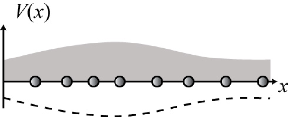
Figure 13: The Fourier component of the random potential $V(x)$ with wavevector small compared to the inverse particle distance act as a random chemical potential. This term increases or decreases smoothly the density. For weak disorder this term does not lead to any localization of the bosons and does not affect the currents or the superfluid correlations. For the TG limit, it would be the equivalent of the forward scattering for the Fermions (see text). The density is indicated by the gray area, while a schematic position of the bosons is given.

Note that the coefficient that relates the change of density to the change of potential is of course the compressibility of the bosons, which is now finite due to the interactions. This term is thus a very classical effect where the bosons go in puddles in the holes of the random potential.

The oscillations at $q\sim 2\pi\rho_{0}$ of the density are deeply affected. In the pure system these correlations were decaying as a powerlaw. Now they behave as

$$\langle e^{i2\phi(x,\tau)}e^{-i2\phi(y,\tau^{\prime})}\rangle\to e^{i\frac{2K}{u}\int_{y}^{x}dzV(z)}\langle e^{i2\phi(x,\tau)}e^{-i2\phi(y,\tau^{\prime})}\rangle_{\rm pure}$$ (74)

If one takes a gaussian disorder with a distribution

$$p(V(x))\propto e^{-D_{f}^{{}^{-}1}\int dxV(x)^{2}}$$ (75)

which leads to averages such as $\overline{V(x)V(x^{\prime})}=D_{f}\delta(x-x^{\prime})$, then the average of the expression 74) gives

$$e^{-\frac{DK^{2}}{u^{2}}|x-y|}\langle e^{i2\phi(x,\tau)}e^{-i2\phi(y,\tau^{\prime})}\rangle_{\rm pure}$$ (76)

leading to an exponential decay of the correlations of the density waves. This is due to the fact that this disorder introduces a random phase in the position of the oscillations of the density.

Paradoxically such a term does not lead to any localization of the bosons. Indeed if one computes the current of bosons, it is given by $J=\partial_{\tau}\phi$. The transformation (73) thus leaves the current invariant and identical to the ones of pure bosons. From the point of view of the transport the system remains a superfluid. Note also that the field $\theta$ is unchanged by the transformation (73), which means that the superfluid correlations are identical to the ones of the pure system. A particularly transparent interpretation of this term can be inferred by looking at the TG limit, or simply at the comparison between the bosonized expressions for the bosons and the spinless fermions systems. As already noted in the Tonks regime $2\pi\rho_{0}\to 2k_{F}$, where $k_{F}$ is the Fermi wavevector. Such a disorder thus corresponds to forward scattering where a fermion around $\pm k_{F}$ remains around the same point of the Fermi surface. It is now obvious that such a forward scattering cannot essentially change the current and cannot lead to localization.

Much more interesting effects arise from the other term, namely

$$H_{\rm dis}=\int dx\;V(x)\rho_{0}(e^{i(2\pi\rho_{0}x-2\phi(x))}+{\rm h.c.})]$$ (77)

Because $\phi$ is a smooth field it is easy to see that this term corresponds now to coupling of Fourier components of the disorder with components around $q\sim\pm 2\pi\rho_{0}$. One can thus rewrite

$$V(x) = \sum_{k}V_{k}e^{ikx}$$ (78)

$$= \sum_{|q|\ll Q}V_{Q+q}e^{i(q+Q)x}+{\rm h.c.}$$

$$= e^{iQx}\xi(x)+{\rm h.c.}$$

where $Q=2\pi\rho_{0}$ and the above equation defines $\xi(x)$. Contrarily to $V(x)$ $\xi(x)$ is a smooth field with averages over disorder of the form

$$\begin{split}\overline{\xi(x)\xi^{*}(y)}&=D_{\rm b}\delta(x-y)\\ \overline{\xi(x)\xi(y)}&=0\end{split}$$ (79)

If $\xi(x)$ was simply constant, (77) would correspond to a commensurate periodic potential, and one would be back to the case of the Mott transition explained in the previous section. The fact that $V(x)$ is random makes the phase of the periodic modulation vary from different positions. We thus see that for the quantum system of bosons, this component of the disorder acts a little bit in a similar way than a periodic potential, trying to pin the charge density wave of bosons. However, because of these phases fluctuations the pinning is not perfect and varies from place to place, leading to a distorted charge modulation. This is shown in Fig. 14.

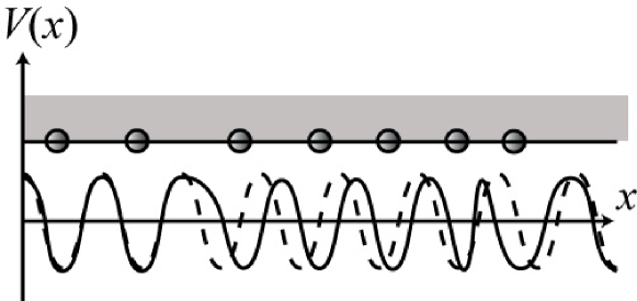
Figure 14: The Fourier components of the disorder $V(x)$ with wavevector close to $Q=2\pi\rho_{0}$ is the one responsible for the localization and the formation of the Bose glass. The full line shows the disorder, while the dashed line would be a periodic potential of wavevector $Q$. The disorder matches the periodicity of the bosons, thus acting in a similar way than a Mott potential, but different portions of the system are shifted compared to the perfect periodic position. Thus although there is pinning of the bosons, the density arrangement is not perfect. Note that for this disorder the smeared density at wavelengthes much smaller than $Q$ is essentially constant as indicated by the gray box. This mechanism of localization is thus quite different than the simple formation of puddles of bosons.

One can also get a simple interpretation for this term by going to the Tonks limit. Indeed in that case this term represents a scattering by the disorder with a momentum close to $\pm 2k_{F}$. It is thus a backscattering term, where a right moving fermion is transformed into a left moving one and vice versa. It is thus clear that such a term affects the current. Exact solutions for noninteracting fermions indeed shows that this term is the one responsible for Anderson localization.

In order to solve for the generic boson system, we can, as for the Mott transition, write the renormalization equations for the disorder and the interactions. The procedure to obtain them is detailed in Giamarchi and Schulz (1988); Giamarchi (2004a). One finds.

$$\begin{split}\frac{dK}{dl}&=-\frac{K^{2}}{2}{\tilde{D}}_{\rm b}\\ \frac{dD}{dl}&=(3-2K){\tilde{D}}_{\rm b}\end{split}$$ (80)

where ${\tilde{D}}_{\rm b}=D_{\rm b}/(\pi^{2}u^{2}\rho_{0})$ and $D_{\rm b}$ is the backward scattering.

The phase diagram can be extracted from these equations, exactly in the same spirit than what was done for the Mott transition in the previous section. The disorder is irrelevant for $K>3/2$, that is, weakly repulsive bosons. One finds a localized phase for $K<3/2$, that is, if the repulsion between the bosons is strong enough. On the separatrix between the two phases the parameter $K$ takes the universal value $K^{*}=3/2$. Thus, the correlation functions decay with universal exponents. For example, the single-particle correlation function decays with an exponent $1/3$. This calculation thus point out the existence for the bosons of a localized phase. This phase, nicknamed Bose glass, whose existence can be established microscopically in one dimension Giamarchi and Schulz (1988) has been generalizable to higher dimensions as well Fisher et al. (1989). In one dimension, one can compute the critical properties of the transition between the superfluid and the Bose glass. I refer the reader to Giamarchi and Schulz (1988); Giamarchi (2004a) for more details on that point. In particular the superfluid stiffness ${\mathcal{D}}$ jumps discontinuously to zero in the Bose glass phase and ${\mathcal{D}}/u=K$ takes the universal value $3/2$ at the transition. At the transition the disorder is marginal. Because of the dual nature of the phases $\phi$ and $\theta$ the fact that the phase $\phi$ is now pinned means that the superfluid correlations decay exponentially, with a characteristic length that is the localization length. One thus expects a lorentzian shape for the $n(k)$ instead of the divergent powerlaw behavior of a Luttinger liquid. The correlation length diverges at the transition to the superfluid phase. Other methods can be used to extract information on the localized phase Giamarchi and Orignac (2003).

This transition from the superfluid to the Bose glass is a direct consequence of the interaction effects between the bosons. In particular the fact that one has a strongly correlated system is hidden in the conjugation relation between the phase $\phi$ and $\theta$ which forces the density fluctuations to be directly related to the superfluid ones. In higher dimensions, although the excitations of the superfluid phase $\theta$ can be described by sound waves, this would not imply much for the fluctuations of the density. In the Bose glass phase, the localization is very similar to the one for spinless fermions. The bosonic nature of the particles is not so important any more. To summarize, in order to be able to observe the localization for quantum interacting bosons, it is important to fulfill the following conditions

1. Have a disorder with sizeable Fourier component close to the interboson periodicity. Having a too smooth potential is of little help, since it can lead to some puddle separation if the disorder is strong but this is a very “classical localization”. The Bose glass phase can also occur for weak disorder.

2. Have repulsive enough interactions between bosons. If $K<3/2$ even an infinitesimal disorder is able to localize. Of course one wants the localization length to be smaller than the size of the system, to observe the localization. The larger the disorder, the larger of course the value of $K$ at which the system localizes. One does not want to make the disorder too strong though (not stronger than the chemical potential) otherwise one is back to the puddle localization mentioned above.

How to reach such limits in a realistic cold atomic system is of course a very challenging question. Current system seem not one dimensional enough and/or with too smooth disorder to be in this quantum limit Clement et al. (2005). One is close however and there is thus little doubts that such a state will be reached in a near future.

There are many directions in which these questions of disorder acting on bosonic systems can be further studied. First for the disordered problem numerical studies have confirmed the analytical predictions and allowed to further study the phase diagram directly in terms of the microscopic parameters Scalettar et al. (1991); Krauth et al. (1991); Rapsch et al. (1999). It is clear that similar studies taking into account the peculiarities of the system (trap etc.) would be very interesting in the context of cold atomic gases.

Second, in the previous section we saw the effect of a periodic potential. We saw that it is very efficient into opening a gap and leading to a Mott insulating phase, but only if the filling is commensurate with the periodicity. On the other hand, a random potential is slightly efficient in giving an insulating phase, but can act regardless of the density of bosons. A particularly interesting intermediate case is the case of quasi-periodic potentials. These potentials lead to a new universality class for the superfluid-insulator transition Vidal et al. (1999); Hida (2000). Similarly one expects very interesting effects when combining disorder and commensurability Fisher et al. (1989); Scalettar et al. (1991); Giamarchi et al. (2001) or going for more than one bosonic mode inside the tube. I refer for example the reader to the literature for other examples of interesting problems such as going to systems of coupled chains Orignac and Giamarchi (1998); Donohue and Giamarchi (2001). It will be very interesting to see if some of these effects can be directly tested in a cold atomic gas context.

6 Conclusions and perspectives

I have shown in these brief notes some of the properties of interacting particles in one dimension. I have focussed principally on interacting one dimensional bosons. Many more examples both on bosons and on other systems can be found in Giamarchi (2004a). Among the many efficient methods both analytical and numerical to tackle one dimensional systems, I have chosen to present here a short account the bosonization method. It is one of the most versatile and physically transparent method. In addition to providing direct insight on the low energy properties of the system, it can also complement very well other angles of approach such as numerical ones. Here again the avid reader will find other methods explained in Giamarchi (2004a). I have shown application of this method to two problems of importance in the rapidly growing field of cold atoms in optical lattices: the Mott transition induced by the presence of a periodic potential on interacting bosons, and the localization of interacting bosons in the presence of a random potential.

Despite an history of more than 40 years the one dimensional world thus continues to offer fascinating challenges. In that respect cold atomic gases have opened a cornucopia of possibilities to test for this fascinating physics. This is due both to the level of control offered by such system but also by their ability to deal with bosons, fermions or mixtures of them at will. It is clear that they have raised many more questions than the theorist had answers ready for, hence offering new playgrounds and challenges. Under such an experimental pressure, there is thus little doubts that one can expect spectacular progress in the years to come.

References

- Emery (1979) Emery, V. J., Plenum Press, New York and London, 1979, p. 247.
- Sólyom (1979) Sólyom, J., Adv. Phys., 28, 209 (1979).
- Voit (1995) Voit, J., Rep. Prog. Phys., 58, 977 (1995).
- Schulz (1995) Schulz, H. J., “Fermi liquids and non–Fermi liquids,” in Mesoscopic Quantum Physics, Les Houches LXI, edited by E. Akkermans, G. Montambaux, J. L. Pichard, and J. Zinn-Justin, Elsevier, Amsterdam, 1995, p. 533.
- von Delft and Schoeller (1998) von Delft, J., and Schoeller, H., Ann. Phys., 7, 225 (1998).
- Schönhammer (2002) Schönhammer, K., J. Phys. C, 14, 12783 (2002).
- Senechal (2003) Senechal, D., in Theoretical Methods for Strongly Correlated Electrons, edited by D. Sénechal et al., CRM Series in Mathematical Physics, Springer, New York, 2003, cond-mat/9908262.
- Gogolin et al. (1999) Gogolin, A. O., Nersesyan, A. A., and Tsvelik, A. M., Bosonization and Strongly Correlated Systems, Cambridge University Press, Cambridge, 1999.
- Giamarchi (2004a) Giamarchi, T., Quantum Physics in One Dimension, Oxford University Press, Oxford, 2004a.
- Takahashi (1999) Takahashi, M., Thermodynamics of One-Dimensional Solvable Models, Cambridge University Press, Cambridge, 1999.
- rev (2004) (2004), for recent reviews on organics, see the volume 104 of Chemical Reviews.
- Dagotto and Rice (1996) Dagotto, E., and Rice, T. M., Science, 271, 5249 (1996).
- Fisher and Glazman (1997) Fisher, M. P. A., and Glazman, L. I., in Mesoscopic Electron Transport, edited by L. Kowenhoven et al., Kluwer Academic Publishers, Dordrecht, 1997, cond-mat/9610037.
- Fazio and van der Zant (2001) Fazio, R., and van der Zant, H., Phys. Rep., 355, 235 (2001).
- Wen (1995) Wen, X. G., Adv. Phys., 44, 405 (1995).
- Dresselhaus et al. (1995) Dresselhaus, M. S., Dresselhaus, G., and Eklund, P. C., Science of Fullerenes and Carbon Nanotubes, Academic Press, San Diego, CA, 1995.
- Pitaevskii and Stringari (2003) Pitaevskii, L., and Stringari, S., Bose-Einstein Condensation, Clarendon Press, Oxford, 2003.
- Greiner et al. (2002) Greiner, M., Mandel, O., Esslinger, T., Hänsch, T. W., and Bloch, I., Nature, 415, 39 (2002).
- Lieb and Liniger (1963) Lieb, E. H., and Liniger, W., Phys. Rev., 130, 1605 (1963).
- Olshanii (1998) Olshanii, M., Phys. Rev. Lett., 81, 938 (1998).
- Stöferle et al. (2004) Stöferle, T., Moritz, H., Schori, C., Köhl, M., and Esslinger, T., Phys. Rev. Lett., 92, 130403 (2004).
- Kinoshita et al. (2004) Kinoshita, T., Wenger, T., and Weiss, D. S., Science, 305, 1125 (2004).
- Paredes et al. (2004) Paredes et al., B., Nature, 429, 277 (2004).
- Jaksch et al. (1998) Jaksch, D., Bruder, C., Cirac, J. I., Gardiner, C. W., and Zoller, P., Phys. Rev. Lett., 81, 3108 (1998).
- Ziman (1972) Ziman, J. M., Principles of the Theory of Solids, Cambridge University Press, Cambridge, 1972.
- Zwerger (2003) Zwerger, W., J. Opt. B: Quantum Semiclass. Opt., 5, 9 (2003).
- Petrov et al. (2000) Petrov, D. V., Walraven, J., and Shlyapnikov, G. V., Phys. Rev. Lett., 85, 3745 (2000).
- Girardeau (1960) Girardeau, M., J. Math. Phys., 1, 516 (1960).
- Haldane (1981a) Haldane, F. D. M., Phys. Rev. Lett., 47, 1840 (1981a).
- Cazalilla (2004a) Cazalilla, M. A., J. Phys. B, 37, S1 (2004a).
- Haldane (1981b) Haldane, F. D. M., J. Phys. C, 14, 2585 (1981b).
- Mahan (1981) Mahan, G. D., Many Particle Physics, Plenum, New York, 1981.
- Cazalilla (2002) Cazalilla, M. A., Europhys. Lett., 59, 793 (2002).
- Nozieres (2004) Nozieres, P., J. Low Temp. Phys, 137, 45 (2004).
- Iucci et al. (2006) Iucci, A., Cazalilla, M. A., Ho, A. F., and Giamarchi, T., Phys. Rev. A, 73, 041608 (2006).
- Cazalilla et al. (2006) Cazalilla, M. A., Ho, A. F., and Giamarchi, T. (2006), cond-mat/0605419; submitted to NJP.
- Mikeska and Schmidt (1970) Mikeska, H. J., and Schmidt, H., J. Low Temp. Phys, 2, 371 (1970).
- Cazalilla (2004b) Cazalilla, M. A., Phys. Rev. A, 70, 041604 (2004b).
- Fisher et al. (1989) Fisher, M. P. A., Weichman, P. B., Grinstein, G., and Fisher, D. S., Phys. Rev. B, 40, 546 (1989).
- Scalettar et al. (1991) Scalettar, R. T., Batrouni, G. G., and Zimányi, G. T., Phys. Rev. Lett., 66, 3144 (1991).
- Giamarchi (1992) Giamarchi, T., Phys. Rev. B, 46, 342 (1992).
- Giamarchi (1997) Giamarchi, T., Physica B, 230-232, 975 (1997).
- Büchler et al. (2003) Büchler, H. P., Blatter, G., and Zwerger, W., Phys. Rev. Lett., 90, 130401 (2003).
- Mott (1949) Mott, N. F., Proc. Phys. Soc. Sect. A, 62, 416 (1949).
- Mott (1990) Mott, N. F., Metal–Insulator Transitions, Taylor and Francis, London, 1990.
- Georges et al. (1996) Georges, A., Kotliar, G., Krauth, W., and Rozenberg, M. J., Rev. Mod. Phys., 68, 13 (1996).
- Imada et al. (1998) Imada, M., Fujimori, A., and Tokura, Y., Rev. Mod. Phys., 70, 1039 (1998).
- Dzyaloshinskii and Larkin (1972) Dzyaloshinskii, I. E., and Larkin, A. I., Sov. Phys. JETP, 34, 422 (1972).
- Kosterlitz (1974) Kosterlitz, J. M., J. Phys. C, 7, 1046 (1974).
- Giamarchi (1991) Giamarchi, T., Phys. Rev. B, 44, 2905 (1991).
- Japaridze and Nersesyan (1978) Japaridze, G. I., and Nersesyan, A. A., JETP Lett., 27, 334 (1978).
- Pokrovsky and Talapov (1979) Pokrovsky, V. L., and Talapov, A. L., Phys. Rev. Lett., 42, 65 (1979).
- Schulz (1980) Schulz, H. J., Phys. Rev. B, 22, 5274 (1980).
- Haldane et al. (1983) Haldane, F. D. M., Bak, P., and Bohr, T., Phys. Rev. B, 28, 2743 (1983).
- Rigol and Muramatsu (2005) Rigol, M., and Muramatsu, A., Phys. Rev. A, 72, 013604 (2005).
- Kollath et al. (2004) Kollath, C., Schollwöck, U., von Delft, J., and Zwerger, W., Phys. Rev. A, 69, 031601(R) (2004).
- Wessell et al. (2004) Wessell, S., Alet, F., Troyer, M., and Batrouni, G. G., Phys. Rev. A, 70, 053615 (2004).
- Pedri and Santos (2003) Pedri, P., and Santos, L., Phys. Rev. Lett., 91, 110401 (2003).
- Gangardt (2004) Gangardt, D. M., J. Phys. A, 37, 9335 (2004).
- Richard et al. (2003) Richard, S., Gerbier, F., Thywissen, J. H., Hugbart, M., Bouyer, P., and Aspect, A., Phys. Rev. Lett., 91, 010405 (2003).
- Altman et al. (2004) Altman, E., Demler, E., and Lukin, M. D., Phys. Rev. A, 70, 013603 (2004).
- Fölling et al. (2005) Fölling, S., Gerbier, F., Widera, A., Mandel, O., Gericke, T., and Bloch, I., Nature, 434, 481 (2005).
- Schori et al. (2004) Schori, C., Stöferle, T., Moritz, H., Köhl, M., and Esslinger, T., Phys. Rev. Lett., 93, 240402 (2004).
- Batrouni et al. (2005) Batrouni, G. G., Assaad, F. F., Scalettar, R. T., and Denteneer, P. J. H., Phys. Rev. A, 72, 031601(R) (2005).
- Reischl et al. (2005) Reischl, A., Schmidt, K. P., and Uhrig, G. S., Phys. Rev. A, 72, 063609 (2005).
- Kollath et al. (2006) Kollath, C., Iucci, A., Giamarchi, T., Hofstetter, W., and Schollwoeck, U. (2006), cond-mat/0603721.
- Giamarchi (2004b) Giamarchi, T., Chem. Rev., 104, 5037 (2004b).
- Arrigoni (2000) Arrigoni, E., Phys. Rev. B, 61, 7909 (2000).
- Georges et al. (2000) Georges, A., Giamarchi, T., and Sandler, N., Phys. Rev. B, 61, 16393 (2000).
- Biermann et al. (2001) Biermann, S., Georges, A., Lichtenstein, A., and Giamarchi, T., Phys. Rev. Lett., 87, 276405 (2001).
- Cazalilla et al. (2005) Cazalilla, M. A., Ho, A. F., and Giamarchi, T., Phys. Rev. Lett., 95, 226402 (2005).
- Ho et al. (2004) Ho, A. F., Cazalilla, M. A., and Giamarchi, T., Phys. Rev. Lett., 92, 130405 (2004).
- Köhl et al. (2004) Köhl, M., Moritz, H., Stöferle, T., Schori, C., and Esslinger, T., J. of Low Temp. Phys., 138, 635 (2004).
- Anderson (1958) Anderson, P. W., Phys. Rev., 109, 1492 (1958).
- Bergmann (1984) Bergmann, G., Phys. Rep., 107, 1 (1984).
- Abrahams et al. (1979) Abrahams, E., Anderson, P. W., Licciardello, D. C., and Ramakrishnan, T. V., Phys. Rev. Lett., 42, 673 (1979).
- Altshuler and Aronov (1985) Altshuler, B. L., and Aronov, A. G., in Electron–electron interactions in disordered systems, edited by A. L. Efros and M. Pollak, North-Holland, Amsterdam, 1985.
- Finkelstein (1984) Finkelstein, A. M., Z. Phys. B, 56, 189 (1984).
- Giamarchi and Schulz (1988) Giamarchi, T., and Schulz, H. J., Phys. Rev. B, 37, 325 (1988).
- Giamarchi and Orignac (2003) Giamarchi, T., and Orignac, E., in Theoretical Methods for Strongly Correlated Electrons, edited by D. Sénechal et al., CRM Series in Mathematical Physics, Springer, New York, 2003, cond-mat/0005220.
- Clement et al. (2005) Clement, D., Varon, A. F., Hugbart, M., Retter, J. A., Bouyer, P., Sanchez-Palencia, L., Gangardt, D. M., Shlyapnikov, G. V., and Aspect, A., Phys. Rev. Lett., 95, 170409 (2005).
- Krauth et al. (1991) Krauth, W., Trivedi, N., and Ceperley, D., Phys. Rev. Lett., 67, 2307 (1991).
- Rapsch et al. (1999) Rapsch, S., Schollwock, U., and Zwerger, W., Europhys. Lett., 46, 559 (1999).
- Vidal et al. (1999) Vidal, J., Mouhanna, D., and Giamarchi, T., Phys. Rev. Lett., 83, 3908 (1999).
- Hida (2000) Hida, K., J. Phys. Soc. Jpn., 69, 311 (2000).
- Giamarchi et al. (2001) Giamarchi, T., Le Doussal, P., and Orignac, E., Phys. Rev. B, 64, 245119 (2001).
- Orignac and Giamarchi (1998) Orignac, E., and Giamarchi, T., Phys. Rev. B, 57, 11713 (1998).
- Donohue and Giamarchi (2001) Donohue, P., and Giamarchi, T., Phys. Rev. B, 63, 180508(R) (2001).