Ground state properties of two spin models with exactly known ground states on the square lattice

Abstract

We introduce a new two-dimensional model with diagonal four spin exchange and an exactly known ground-state. Using variational ansätze and exact diagonalisation we calculate upper and lower bounds for the critical coupling of the model. Both for this model and for the Shastry–Sutherland model we study periodic systems up to system size $6\times 6$.

I Introduction

In this paper we study two frustrated two-dimensional quantum spin models with exactly known singlet dimer ground states.

First we consider the Shastry–Sutherland model ShSu , a two dimensional Heisenberg model with an additional frustrating coupling of strength $J_{1}$ on every second diagonal bond (see Fig.1) with Hamiltonian

$$H = J_{2}\sum_{<i,j>}{\vec{S}_{i}\vec{S}_{j}}+J_{1}\sum_{<i,j>diagonal}{\vec{S}_{i}\vec{S}_{j}}.$$ (1)

Though the model shows similar properties also for higher spins, here we restrict ourselves to the case of spin $\frac{1}{2}$, and the $\vec{S}_{i}$ denote spin-1/2 spin operators located at site $i$. The model Eq.1 has attracted attention recently, when it was suggested, that the magnetic properties of the substance SrCu₂(BO₃)₂ Kage are very well described by its frustrated spin-spin interactions.

The second model we investigate incorporates a diagonal ring exchange term on every second plaquette (see Fig.2). It is given by the Hamiltonian

$$H = J_{2}\sum_{<i,j>}{\vec{S}_{i}\vec{S}_{j}}+J_{1}\sum_{plaquette\ k}({\frac{3}{4}+\vec{S}_{k_{1}}\vec{S}_{k_{3}}})({\frac{3}{4}+\vec{S}_{k_{2}}\vec{S}_{k_{4}}})$$ (2)

where again the $\vec{S}_{i}$ denote spin-1/2 spin operators and the second sum runs over every second plaquette $k$ as depicted in Fig.2. The four-spin interaction is normalized in such a manner that the dimer ground states, which play a major role in what follows, have zero energy. The extra four spin interaction of Eq.2 can be viewed as a “truncated” version of the ring exchange which has been discussed in the context of the two-dimensional mother substances of High $T_{c}$ Coldea and which have been found to play an essential role in spin ladder substances like Sr₁₄Cu₂₄O₄₁ Schmi .

Both models display rich phase diagrams and both have exactly known singlet dimer ground states. The latter property is otherwise rarely encountered when dealing with two-dimensional quantum spin systems: The ground state of the Shastry–Sutherland model is non degenerate and consists of (singlet) dimers located along the diagonal bonds, for the plaquette model the corresponding ground state is two-fold degenerate, and each ground state corresponds to a covering of the two types of diagonals with dimers.

To facilitate the following discussion we define for both models the variable $x:=J_{2}/J_{1}$, which can be viewed as an inverse frustration. The models undergo a zero temperature first order phase transition to the exactly known singlet dimer state at a critical inverse frustration $x_{c}$. The numerical value of $x_{c}$ is different for the two models.

The aim of this paper is to introduce the basic properties of the plaquette model and to determine the value of $x_{c}$ with best possible accuracy for both the Shastry–Sutherland and the plaquette model. Hereby we want to demonstrate, that also for two-dimensional frustrated models which are hard to tackle numerically, by use of the Lanczos technique on finite clusters not only reliable but also precise results for the infinite system can be obtained. We also hope, that our results are of use to gauge methods using uncontrolled approximations, whose errors are usually hard to assess.

The paper is organized as follows. Sect.II is devoted to a study of the plaquette model using variational methods and finite cluster analysis. In particular two types of variational ansätze are used to give upper and lower bounds for the model s critical coupling $x_{c}$. In Sect.III.1 we present a study of the Shastry–Sutherland model of unprecedented precision using the Lanczos algorithm for system sizes up to $6\times 6$ with periodic boundary conditions. In Sect.III.2 we present a similar analysis for the plaquette model on periodic systems and give a comparison of the two models. In Sect.IV we summarize our results and give an outlook to future possibilities.

Figure 1: Shastry–Sutherland model with $J_{2}$ along diagonal bonds and $J_{1}$ along vertical and horizontal bonds. The dimer ground state is build up by dimers i.e. $\frac{1}{\sqrt{2}}(\uparrow\downarrow-\downarrow\uparrow)$ pairs along the diagonal bonds.

Figure 2: Plaquette model with four spin interaction.

Figure 3: Ground state phase diagram of the plaquette model. The phase boundaries between the dimer and the Néel phase is drawn at $J_{2}=J_{1}/2$ which corresponds to a system with $N=4$ spins.

Figure 4: $x_{c}$ calculated on finite clusters with open boundary conditions for the Shastry–Sutherland model Eq.1 and the plaquette model Eq.2. The values for the Shasty–Sutherland model are taken from Ref.us and are listed here for comparison.

Figure 5: A variational configuration of the ”good type”, consisting of two empty plaquettes with four spins and a four spin exchange between the plaquettes, gives an upper bound of $\frac{31}{48}$. For a corresponding configuration of the Shastry–Sutherland model us one obtains an upper bound of $\frac{3}{4}$, wheras a configuration with the diagonal coupling $J_{1}$ on the plaquettes (”bad type”) gives only $\frac{7}{8}$ as upper bound.

Figure 6: $x_{c}$ calculated on finite clusters with periodic boundary conditions for the Shastry–Sutherland model Eq.1 and the plaquette model Eq.2.

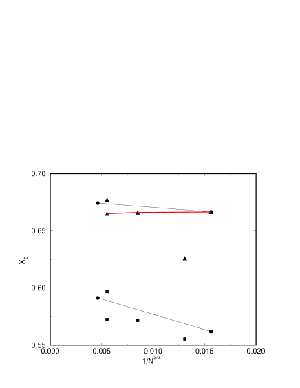
Figure 7: $x_{c}$ plotted versus $1/N^{3/2}$ for the Shastry–Sutherland model Eq.1 (triangles and circles) and for the plaquette model Eq.2 (squares and circles). The lines connect systems with the same shape

II The Plaquette model

II.1 The ground state phase diagram

Some first insight in the model can be gained by considering the smallest possible cluster, which consists of a plaquette of four spins only. This system has two singlet eigenstates with spin $S=0$, three triplets with $S=1$, and one “ferromagnetic” state with $S=2$. The ground state diagram can be easily drawn for this system (see Fig.3). Moving from the singlet dimer phase in anticlockwise direction at $x=\frac{J_{2}}{J_{1}}=\frac{1}{2}$ one enters a second singlet phase usually referred to as antiferromagnetic phase or Néel phase and at $J_{2}=0,J_{1}<0$ starts the ferromagnetic phase, which at $x=-1$ meets again the singlet dimer phase. For $N=4$ the singlet dimer phase is degenerate with two $S=1$ phases. The third $S=1$ state is a ground state only for $J_{2}=0$ and $J_{1}<0$, where it is degenerate with the Néel and the ferromagnetic state.

It is still an open question to what extent a third phase phase between the dimer and the Néel phase exists for the infinite system. This problem is similar to the still unsolved issue in the Shastry–Sutherland model, for which various scenarios of intermittent phases between the Néel phase and the singlet dimer phase have been discussed.

The phase boundaries between the Néel phase and the ferromagnetic phase and between the ferromagnetic and the dimer phase are exact, i.e. they coincide with the boundaries of the infinite system. However the value $x^{(N=4)}_{c}=0.5$ of the phase boundary between the dimer and its adjacent phase is not correct for the infinite lattice. To determine the value of $x_{c}$ also for the infinite lattice, we calculated both lower and upper bounds and also study finite clusters with periodic boundary conditions.

II.2 Lower and upper bounds for the Plaquette model

Using variational ansätze in Ref.us lower and upper bounds for the critical values $x_{c}$ were discussed for the Shastry–Sutherland model. Here we perform a similar analysis for the plaquette model. As was pointed out by P.W. Anderson Anderson the ground state energy of open clusters $H_{i}$ with no overlapping bonds, which cover the whole plane, represent a lower bound for the ground state energy of the infinite system. Similar to the Shastry–Sutherland system we can infer thus from the 4 spin plaquette that $x^{(4)}_{c}=0.5$ is a lower bound for $x_{c}$ of the infinite system. An analysis of systems of larger size (see Fig.4) gives as best lower bound $x_{c}>0.54263$, which is the critical coupling of an open system of size $N=31$. Unfortunately the unsystematic variation of the bound with the system size does not allow a meaningful extrapolation.

To obtain an upper bound on the critical coupling $x_{c}$ the Hamiltonian is split into clusters without common spins and into external bonds connecting the clusters

$$H=\sum_{cluster}H_{cluster}^{N}+H_{bond}.$$ (3)

This is graphically depicted in Fig.5 for clusters with four spins. As variational state we use a product state $\prod_{cluster}|\Psi_{cl}\rangle$, where $|\Psi_{cl}\rangle$ is the ground state of the cluster with Hamiltonian $H_{cluster}^{N}$. In contrast to the Shastry–Sutherland model however, where the expectation value of the external bonds vanishes for the ground state, which has spin $S=0$, in case of the plaquette model the expectation value

$$\langle\prod_{cluster}\Psi_{cl}|H_{bond}|\prod_{cluster}\Psi_{cl}\rangle$$ (4)

has to be explicitly evaluated. Again a first bound can be found by considering clusters of size $N=4$. Best results are obtained here by using a plaquette with no four spin interaction as basic cluster (as shown in Fig.5). One thus obtains $x_{c}<\frac{31}{48}\approx 0.6458$. Again the numerical value can be improved here by considering larger clusters. Since the situation is more complicated in the case of the plaquette model, because one needs to consider also the bonds, we restrict ourselves here to a square lattice of size $N=16$, from which a numerical diagonalisation gives $x_{c}<0.627(1)$.

To conclude, we find $0.54263<x_{c}<0.627(1)$ as exact bounds on the critical coupling of the plaquette model.

III The Shastry–Sutherland and the plaquette model on systems with periodic boundary conditions

III.1 The Shastry–Sutherland model

We do not intend to give a detailed description of the Shastry–Sutherland model here since over the years it has been vastly discussed (see e.g. ShSu ; Kage ). In this paper we summarise only briefly the results on $x_{c}$, which are most relevant for our work based on Lanczos technique Lan .

Using variational approaches us it can be inferred from clusters of 31 and 32 sites, that $0.5914<x_{c}<0.6955$. Thus by calculating variational bounds the margin left open for $x_{c}$ is approximately 0.1.

In this paper we discuss finite systems with periodic boundary conditions, which usually are closer to the infinite size system than systems with open boundaries. Also they allow to study larger systems, because translational invariance can be used to further reduce the size of the subspaces (for a list of the symmetries used for the different systems see table 3).

Here we concentrate in particular on a precise determination of the critical coupling of a $6\times 6$ system. To successfully study this problem we had to deal with subspaces of dimension $5\cdot 10^{8}$. We accomplished this by using parallel OpenMP programming techniques. We also investigated a $N=32$ square system and periodically closed $4\times n$ systems with up to $n=8$. An overview of all the clusters with periodic boundaries is given in Fig.6. Our results for the $6\times 6$ system are shown in table 2 and for the $N=32$ square systems in table 1.

As a technical point we mention that except for the trivial case of $N=4$, there is no argument why the ground state energy for $x>x_{c}$ should be linear in $x$. To obtain optimal results we have therefore chosen values of $x$ as close as possible to $x_{c}$ (see table 1 and 2). This is most important for the $N=36$ system, for which calculating extra points is time consuming. We thus find as result for $N=36$ a critical value of $x_{c}=0.674408$, for the $32$ square we obtain $x_{c}=0.67724$ and for the $4\times 8$ stripe $x_{c}=0.66509$. More values for smaller systems can be found in Fig.6.

When studying two-dimensional clusters with periodic boundary conditions it is obvious, that the finite size effects depend not only on the number of spins in the system, but also on the geometry of the clusters. Here we have two types of systems, one consists of the $N=4\times n$ stripes with $N=16,24,32$ spins and square systems with $N=16,36$. As was already pointed out in us the stripe type systems with open boundaries show a linear finite size behaviour in $1/N$. We therefore extrapolate the $N=16,24,32$ stripe systems as a function of $1/N$ and find $x_{c}=0.6624$, which is an extrapolation for the $4\times n-$ stripe, however it cannot be taken as a limit for the two-dimensional system, because we deal essentially with a one-dimensional system.

On first sight it seems a good idea to try an extrapolation of the $N=8,18,32$ systems. This is however not feasible, because the $N=18$ system, has rather pathological periodic boundary conditions and cannot be taken as a square system.

The line connecting the system with $N=16$ and $N=36$ is not an extrapolation, since the dependence on $1/N^{3/2}$, which is motivated by CHN ; HN ; Sandvik is a guess. The line crosses the ordinate at $x_{c}=0.678$, assuming a $1/N$ dependence gives $x_{c}=0.681$ and assuming $1/N^{2}$ yields $x_{c}=0.6764$. All three values lie within the upper and lower bonds from Ref.us .

The fact, that the $x_{c}$ for $N=16$ is smaller than for $N=36$ prompts us to believe that the true $x_{c}$ should be larger than $x_{c}=0.6744$. If true, this means, that the value $x_{c}=0.63$ found by Knetter et. al KnUh using the flow equation method is too small. We roughly agree with the value $x_{c}=0.7\pm 0.01$ from Ref.MiUe , which is obtained by extrapolating results from systems with $4-20$ spins.

III.2 The Plaquette Model

The finite size behaviour of the plaquette model is in many respects similar to the Shastry–Sutherland model. Again the $4\times n$ stripes have lower $x_{c}$ than the two-dimensional systems. Extrapolating the $N=18$ and $N=32$ squares in the above fashion gives $x_{c}=0.627$ which coincides with the upper bound obtained from the $N=16$ system. A $1/N$ dependence is not compatible with the upper bound and a $1/N^{2}$ extrapolation gives $x_{c}=0.616$. It seems more reliable to draw conclusions from the $N=36$ and the $N=16$ system. For the $N=6\times 6$ square system we find $x_{c}=0.59136$, which is again larger than the corresponding $x_{c}=0.56198$ of the $4\times 4$ system. We expect (though again there is no rigorous argument) that the critical coupling of the infinite size system should be larger than $x_{c}=0.59136$. The line connecting the point of the $4\times 4$ and $6\times 6$ when plotted versus $1/N^{3/2}$ crosses the ordinate at $x_{c}=0.603$ (assuming a $1/N$ dependence gives $x_{c}=0.615$ and assuming $1/N^{2}$ yields $x_{c}=0.599$), all values lie between the rigorous upper and lower bonds of Sect.II.

$J_{2}/J_{1}$	$E_{0}/N$	$J_{2}/J_{1}$	$E_{0}/N$
0.67700000	-0.374999999998987	0.45000000	6.99440505513849e-15
0.67720000	-0.374999999999945	0.59000000	1.49880108324396e-15
0.67724000	-0.374999999997117	0.60000000	-0.00136332822402102
0.67724400	-0.374999999997006	0.61000000	-0.00564902914422299
0.67724600	-0.374999999997179
0.67724800	-0.375000015810957
0.67730000	-0.375023759933420
0.67750000	-0.375115180019318
0.67780000	-0.375252606784488
0.68000000	-0.376271688712272
0.70000000	-0.386720856118170

Table 1: Data points calculated for the square $N=32$ Shastry–Sutherland model (left) and plaquette model (right). The dimension of the subspace containing the ground state is $75.164.451$.

$J_{2}/J_{1}$	$E_{0}/N$	$J_{2}/J_{1}$	$E_{0}/N$
0.50000000	-0.374999999999425	0.50000000	8.16485767884956e-13
0.66697792	-0.374999999995975	0.59135000	5.54148393838716e-12
0.67441000	-0.375003966117052	0.59140000	-1.70109703724886e-05
0.67500000	-0.375286177720292	0.59330700	-0.000846068815337997
0.68000000	-0.377704740424690	0.59331000	-0.000847382217467496
0.70000000	-0.388578449404367	0.62000000	-0.0133823277140735
0.80000000	-0.451753105004501	0.63000000	-0.0183954992316725
0.85000000	-0.484334145942023

Table 2: Data points obtained for the $N=6\times 6=36$ Shastry–Sutherland model (left) and plaquette model (right). The dimension of the subspace with the ground state is $504.174.594$.

IV Summary and Outlook

We have introduced a plaquette model with an exactly known ground state and calculated the critical coupling $x_{c}$ of the dimer phase in the model using the Lanczos algorithm for systems up to $N=36$. For a $6\times 6$ system we find $x_{c}=0.59136$, as rigorous bounds for the critical coupling of the infinite system we obtain $0.54263<x_{c}<0.627(1)$.

We also calculated the critical coupling of the Shastry–Sutherland model and obtained $x_{c}=0.6744$ for a system with periodic boundaries and size $N=6\times 6$. Extrapolating two-dimensional systems is subtle. Our best guess for the infinite system is $x_{c}=0.678$ for the Shastry–Sutherland model and $x_{c}=0.603$ for the plaquette model.

We hope that our work will prompt further investigations of the plaquette model, in particular a detailed comparison of the magnetic properties of the plaquette model with the ”full plaquette interaction” expected in high $T_{c}$ mother substances seems an attractive problem.

system	dimension of subspace	$S_{z}$	momentum	reflection	spin inversion
32 square (periodic)	75.164.451	$\times$	$\times$		$\times$
$4\times 8$ (periodic)	37.582.307	$\times$	$\times$		$\times$
$6\times 6$ (periodic)	504.174.594	$\times$	$\times$		$\times$
28 (open)	20.058.300	$\times$			$\times$
31 (open)	150.283.611	$\times$		$\times$

Table 3: Table of the dimensions of the subspaces and symmetry operations, which were implemented for the 32 square, the $4\times 8$ and the $6\times 6$ system with periodic boundaries and for the 28 and 31 systems with open boundaries.

V Acknowledgments

We would like to thank E. Müller-Hartmann for many useful discussions. Most of the data presented were obtained using the supercomputing facility IBM p690 (JUMP) at the John von Neumann Institute for Computing (NIC) at the Forschungszentrum Jülich and the SMP Sun Fire Cluster at the Computing Center of the RWTH Aachen.

References

- (1) B. S. Shastry and B. Sutherland, Physica B 108, 1069 (1981).
- (2) H. Kageyama, K. Yoshimura, R. Stern, N. V. Mushnikov, K. Onizuka, M. Kato, K. Kosuge, C. P. Slichter, T. Goto and Y. Ueda, Phys. Rev. Lett. 82, 3168 (1999).
- (3) R. Coldea et al., Phys. Rev. Lett. 86, 5377 (2001).
- (4) H. J. Schmidt and Y. Kuramoto, Physica B 163, 443 (1990).
- (5) U. Löw, E. Müller-Hartmann, J. Low Temp. Phys. 126, 1135 (2002) and Erratum.
- (6) P. W. Anderson, Phys. Rev. 83, 1260 (1951).
- (7) C. Lanczos, C. Res. Natl. Bur. Stand. 45, 255 (1950).
- (8) J. S. Chakravaty, B. I. Halperin, D. R. Nelson, Phys. Rev. B 39, 2344 (1989).
- (9) P. Hasenfratz, F. Niedermayer, Phys. Lett. B 268, 231 (1991).
- (10) A. W. Sandvik, Phys. Rev. B 56 11678 (1997).
- (11) C. Knetter, A. Bühler, E. Müller-Hartmann, and G. S. Uhrig, Phys. Rev. Lett. 85, 3958 (2000).
- (12) S. Miyahara, and K. Ueda, Phys. Rev. Lett. 82, 3701 (1999).