Transport Processes on Homogeneous Planar Graphs with Scale-Free Loops

Abstract

We consider the role of network geometry in two types of diffusion processes: transport of constant-density information packets with queuing on nodes, and constant voltage-driven tunneling of electrons. The underlying network is a homogeneous graph with scale-free distribution of loops, which is constrained to a planar geometry and fixed node connectivity $k=3$. We determine properties of noise, flow and return-times statistics for both processes on this graph and relate the observed differences to the microscopic process details. Our main findings are: (i) Through the local interaction between packets queuing at the same node, long-range correlations build up in traffic streams, which are practically absent in the case of electron transport; (ii) Noise fluctuations in the number of packets and in the number of tunnelings recorded at each node appear to obey the scaling laws in two distinct universality classes; (iii) The topological inhomogeneity of betweenness plays the key role in the occurrence of broad distributions of return times and in the dynamic flow. The maximum-flow spanning trees are characteristic for each process type.

I Introduction

In recent years an intensive research on networks structure and dynamics recent_review was conducted, motivated both with theoretical reasons and practical applications to improve network’s performance, for instance in the communication networks. It has been recognized that network structure may influence the course of the dynamic processes on it through the topological constraints fixed by network complex patterns of links and higher topological sub-structures. Certain types of processes run better on networks with higher structural complexity we_review ; TT ; TTR , whereas other processes, like synchronization synchronization , are more efficiently accomplished on homogeneous structures. In this respect, a range of structure–function matching possibilities opens, depending on the details of the dynamics BCN_optimization ; Hurtado ; KK .

In the case of transport of information packets two markedly different structures were found BCN_optimization corresponding to minimized travel time of packets: a scale-free structure at low traffic density, and a homogeneous structure at high traffic density. The highly clustered scale-free graph was also found to support efficient free-flow traffic with the local navigation rules compatible with the “information horizon” of the graph TT ; TTR ; TT_05 . The emergent efficiency of transport is related to the central role of the hub and its associated super-structure TTR . However, the structure is vulnerable for jamming when the creation rate exceeds a (large) critical value TT ; TTR . In this regime, a homogeneous network with distributed node activity is expected to perform better BCN_optimization . Apart from the limitation to free graphs (i.e., graphs in the infinite space dimension) and relatively low transparency of the simulated annealing procedure at large networks, the results of Ref. BCN_optimization revealed main structure–traffic interdependences and traced routes towards improved efficiency of transport processes on complex networks. The following questions remain open:

• What topological property on a small scale of the underlying network plays the key role in given dynamics?

• How these globally optimal topologies perform in the case of traffic with constraints of restricted geometries?

Here we address these questions using numerical simulations to study comparatively two types of transport processes on a homogeneous planar graph with scale-free distribution of loops. In particular, we study: (1) Traffic of information packets between specified pairs of nodes on the graph at constant packet density (fixed number of moving packets) $\rho\gg 1$; and (2) Transport of electrons via tunneling between nodes, which are driven by the constant voltage difference $V=const$ on electrodes. In both cases the transported packet (electron) has a specified source and sink as a pair of nodes on the graph. The packets are navigated locally towards their destination (sink) node, whereas the electrons are driven globally by the voltage profile. Another important difference in these processes is that the information packets interact by making queues on a node. In contrast, the number of electrons on a node is practically unrestricted and order of their processing is random. We determine quantitative characteristics of these two processes on the same network (fixed by its adjacency matrix) and attempt to relate the statistical properties of transport to the microscopic process rules. In contrast to the above mentioned networks in infinite dimensional space, we consider here a graph that is constrained to a planar geometry. We also fix the number of links per node to strictly $k=3$, in order to minimize the effects of node connectivity. Our main findings are that in transport on planar graphs the key topological feature is the betweenness centrality of nodes. Different processes utilize the underlying structure in different ways leading to statistically different outcomes. The observed traffic properties can be further related to certain features of the microscopic dynamics, specifically to queuing and driving details.

In Section II we present the graph structure and its main topological characteristics MSBT_iccs06 . Section III defines the transport processes and their numerical implementation on the graph. Main features of the traffic noise are considered in section IV, and relation between the topological and dynamical centrality measures are studied in Section V. Section VI contains a short summary and the discussion of the results.

II Structure

Planar graphs are mathematical objects that can be embedded into an Euclidean plane. They obey the following topological constraints BB_book : A graph is planar iff it does not contain a subdivision of $K_{5}$ (5-clique) and $K_{3,3}$ structures, and the Euler relation $N_{p}+N=E+1$ between the number of polygons $N_{p}$, nodes $N$, and links $E$ is satisfied.

We grow a planar graph by cell aggregation procedure, which we introduced earlier MSBT_iccs06 . Here we observe a strict constraint of node connectivity $k=3$ for all nodes enclosed in the graph interior. The cells are loops of nodes with varying lengths $\ell$ driven from a power-law distribution $P(\ell)\sim\ell^{-\tau}$. The aggregation is starting from an initial loop and nesting additional loops along the boundary of the graph. In order to observe the constraint of maximum connectivity $k=3$, a nesting place along the graph boundary is searched and its length $n_{d}$ is identified as the distance between two successive nodes with connectivity $k=2$. Then the nesting is performed with a probability $p\sim\exp{(-\nu n_{s})}$, where $n_{s}$ represents the excess number of nodes, defined as the difference between current loop length $\ell$ and the length of the selected nesting string $n_{d}$. The number of nodes that are successfully nested are identified with the existing $n_{d}$ nodes along the nesting site on the graph boundary. In this way the parameter $\nu$ plays the role of the chemical potential for addition of nodes. In general, when $\nu$ is small, the probability of adding a large number of new nodes $n_{s}$ attached to a short nesting site is larger, resulting in a more branched graph structures, compared with more homogeneously space-filling loops obtained for large $\nu$ values MSBT_iccs06 . An example of the structure for large $\nu$ and $\tau=2.2$ is shown in Fig. 1 (left).

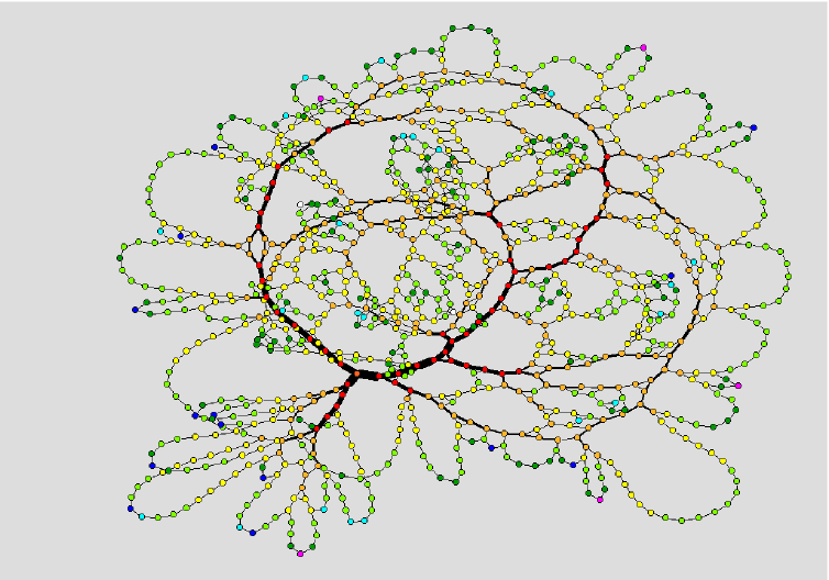
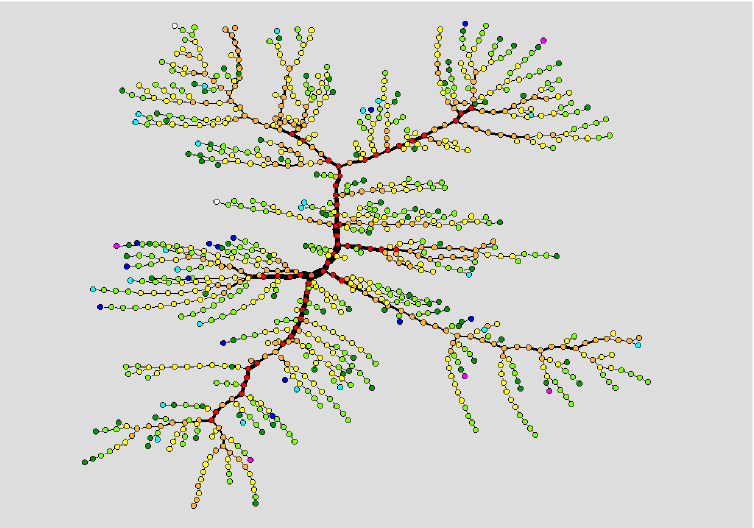
Figure 1: Emergent planar graph with scale-free distribution of loop sizes and nesting potential $\nu=5$ (left) and its maximum-betweenness-spanning tree (right). Line widths indicate relative topological betweenness of links. Different colors are coding the topological centrality of nodes.

It should be stressed that, due to the planar constraints the emergent graph structure is not of a small-world type. In addition, the graph is strictly homogeneous and clustered (probability of a short triangle loop $\ell=3$ is relatively high in the power-law distribution of loops). A remarkable feature of this type of graphs is its inhomogeneity in the betweenness centrality for both nodes and links. In Fig. 1 the centrality of links is marked on the graph with lines of different widths. The topological maximum betweenness spanning tree, in which each node is linked to the rest of the nodes on the graph via its largest betweenness link, is also shown in Fig. 1 (right). Due to graph homogeneous connectivity, the maximum betweenness nodes lie on the maximum betweenness links (see the color-coded figure).

III Dynamics

We consider two types of dynamic processes on the graph shown in Fig. 1 (left): (i) Autonomously driven constant-density transport of information packets (IP) and (ii) Constant-voltage- driven tunneling current (Q). Next we describe the two processes in detail and then determine their statistical properties, in particular features of the traffic noise and dynamical flow. We then discuss the traffic features relative to the topological properties of the graph. The graph (Fig. 1) contains $N=1003$ nodes connected according to its adjacency matrix and is identical in both processes.

III.1 Information Flow at Constant Density

Transport of the information packets on the graph takes part between an in advance specified pair of nodes—origin and destination node of a packet, which are selected randomly. Motion of a packet on the network is implemented as a guided random walk from the origin of the packet towards its destination TT ; TTR ; TT_05 ; BT_ccp03 . At each node the packets are navigated through the graph using the local nnn-search rule, where two depth levels around each node (sometimes called information horizon 2) are searched for the packet destination address TT ; TTR ; TT_05 ; BT_ccp03 . The rule is supplemented by random diffusion when the search is unsuccessful. The whole network is updated in parallel. The packets are removed when they arrive at their destinations. Here we implement the traffic for a fixed number of moving packets. We start with a given number $\rho$ of packets. The arrived and removed packets are replaced in the next time step by creating the same number new ones at randomly chosen nodes and assigned new destinations. In the limit $\rho=1$ this corresponds to the sequential guided random walk problem. For $\rho>1$ packets interact with each other by making queues at nodes along their paths. The queuing of packets is a qualitatively new feature of dense traffic on networks. The packet density is controlled with the number of moving packets $\rho$ on the graph with a fixed number of nodes $N$. We assume finite queue lengths $H=1000$, and a LIFO (last-in-first-out) queuing rule TTR . Details of the numerical implementation can be found in Ref. BT_ccp03 .

III.2 Voltage-Driven Electron Tunneling

Description: In this dynamic process the graph represent system of nano particles (nodes) Philip_SA ; Philip_REP with equal inter-dot capacitances over links, $C$, and equal capacitances between dot and gate, $C_{g}$. We assume conditions that lead to Coulomb-blockade transport nanoarrays_book with equal tunneling resistance $R$. Electrodes are associated to two subsets of the graph boundary nodes. Each electrode length and distance between them is taken as one quarter of the graph boundary length. Total energy of this system can be written as nanoarrays_book ; PRL-93 ; CB

$$E=\frac{1}{2}\mathbf{Q}^{\dagger}M^{-1}\mathbf{Q}+\mathbf{Q}\cdot V^{ext}+Q_{\nu}\Phi^{\nu},$$ (1)

$$V^{ext}=M^{-1}\mathbf{C}_{\nu}\Phi^{\nu},$$ (2)

where $M$ is the capacitance matrix, $\mathbf{Q}$ is the vector of charges on dots, $\Phi^{\nu}$ —potential of an electrode, $\nu\in\{+,-,gate\}$, and $\mathbf{C}_{\nu}$ is the vector of capacitances between dots and electrode $\nu$. The diagonal elements of $\mathbf{M}$ are the sum of all capacitances associated with a dot and off-diagonal elements are the negative interdot capacitances: $M_{ij}=-C_{ij}$, $i\neq j$ and $M_{ii}=\sum_{j}C_{ij}+\sum_{\nu}C_{\nu,i}$, where $C_{ij}$ is the adjacency matrix of the graph.

Dynamics: The single electron tunneling rate through a junction (link) $ij$ is calculated:

$$\Gamma_{ij}=-\frac{\Delta E_{ij}/e^{2}R}{1-\exp({\Delta E_{ij}}/{k_{B}T})},$$ (3)

where $R$ is the quantum tunneling resistance, $\Delta E_{ij}$ is the energy change associated with a tunneling process along the $i\to j$ link, and $k_{B}T$ is the thermal energy. The rate $\Gamma_{ij}$ then determines the probability density function of the tunneling time $t$ by $p_{ij}(t)=\Gamma_{ij}\exp(-\Gamma_{ij}t)$.

Implementation: System is initiated as a network of dots without charges and a voltage difference $V$ between the electrodes is imposed. In each step we compute rates $\Gamma_{ij}$ and determine respective tunneling times from the distribution $p_{ij}(t)$ for all junctions $\{ij\}$. We process a single electron tunneling through the junction that has the shortest tunneling time. After each step we sample time, number of charges on all dots, number of charges that arrived to the zero-voltage electrode (current). We also keep track of number of tunnelings that occurred along each link and on each node.

Parameters and optimization: In all calculations the potential of the gate and on one electrode is kept to zero and constant potential $V$ on the other electrode. The system was on zero temperature. The elements of the inverse capacitance matrix $M^{-1}$ fall off exponentially with a screening length, which is proportional to $C/C_{g}$. We assume $C/C_{g}\ll 1$, which permits computational acceleration by using only nearst-neighbour elements of $M^{-1}$ for calculation of the energy change in Eqs. (1-3). For the same reason, the potential $V^{ext}$ (2) can be considered as a constant within the shortest computed time window $\delta t\sim 1/\Gamma_{max}$.

Non-linearity and statistics: Driven by the external potential, the charges are entering the system from the high-voltage electrode. For small voltage on that electrode, the charges can screen-off the external potential. In that case, after some transient time, the system become static and there is no current. For voltage larger than a threshold voltage $V_{T}$ the screening does not occur and after some transient time a stationary distribution of charges over dots sets-in with a constant current. In general, current-voltage dependence is non-linear PRL-93 ; we-future $I\sim(V-V_{T})^{\zeta}$ for $V>V_{T}$. For this network type we find $\zeta\approx 3$ we-future . In this paper we consider transport properties for a fixed voltage $V=10V_{T}$ in the non-linear regime. The data are collected after the transient time when a constant current occurs.

IV Noise Properties in the Stationary Flow Regime

In the case of electron tunneling with voltage difference $V$ between the electrodes, the distribution of electrons per node in the stationary state is compatible with the actual value of the voltage at that node. An electron moves along a link towards the zero-voltage electrode when the tunneling condition $\Gamma_{ij}>0$, with $\Gamma_{ij}$ in Eq. (3), is satisfied. Thus the number of tunnelings on a node fluctuates in time around an average value which is determined by the voltage profile. We consider the charge fluctuations $Q_{i}(t)$ at a node $i$ as a time-series taken over discrete time points $t/<\Gamma_{max}^{-1}>=1,2,\cdots$.

In the case of information packet transport the stationarity is guaranteed by the implementation of the constant density, here $\rho=100$ packets. (In other driving modes the stationary traffic occurs for posting rates below a certain critical value for each network TT ; TTR .) For a fixed node $i$ on the network, the number of packets arriving to that node $h_{i}(t)$ fluctuates in time steps $t$, depending on the activity of its neighbour nodes. Each node tries to process top packet on it towards packet’s actual destination. Thus a macroscopic current is absent.

Power Spectra. The power spectrum of the corresponding time series is shown in Fig. 2a (bottom line), with the form $S(f)\sim f^{-\phi}$, $\phi\approx 0.9$, within error bars,indicating a long-range correlations for large frequencies. In contrast, the corresponding power-spectrum of the time series collected at the zero-voltage electrode in the tunneling process, which is given in Fig. 2b (lower curve), indicates a white noise. Another time series comprises of the fluctuating number of nodes which are simultaneously processing a packet (electron), $n(t)$. Its power spectrum is also shown in Fig. 2a and b (top curves) for both packet and electron processing, respectively. These series appears to be weakly correlated on the planar graph. Since the network structure is identical in both processes, the observed difference in the noise correlations can be attributed to the interaction mechanisms and driving conditions. In particular, the processed packets interact locally via queuing at a node, whereas number of electrons at each node is determined by global energy minimum conditions, given by the Hamiltonian in Eq. (1).

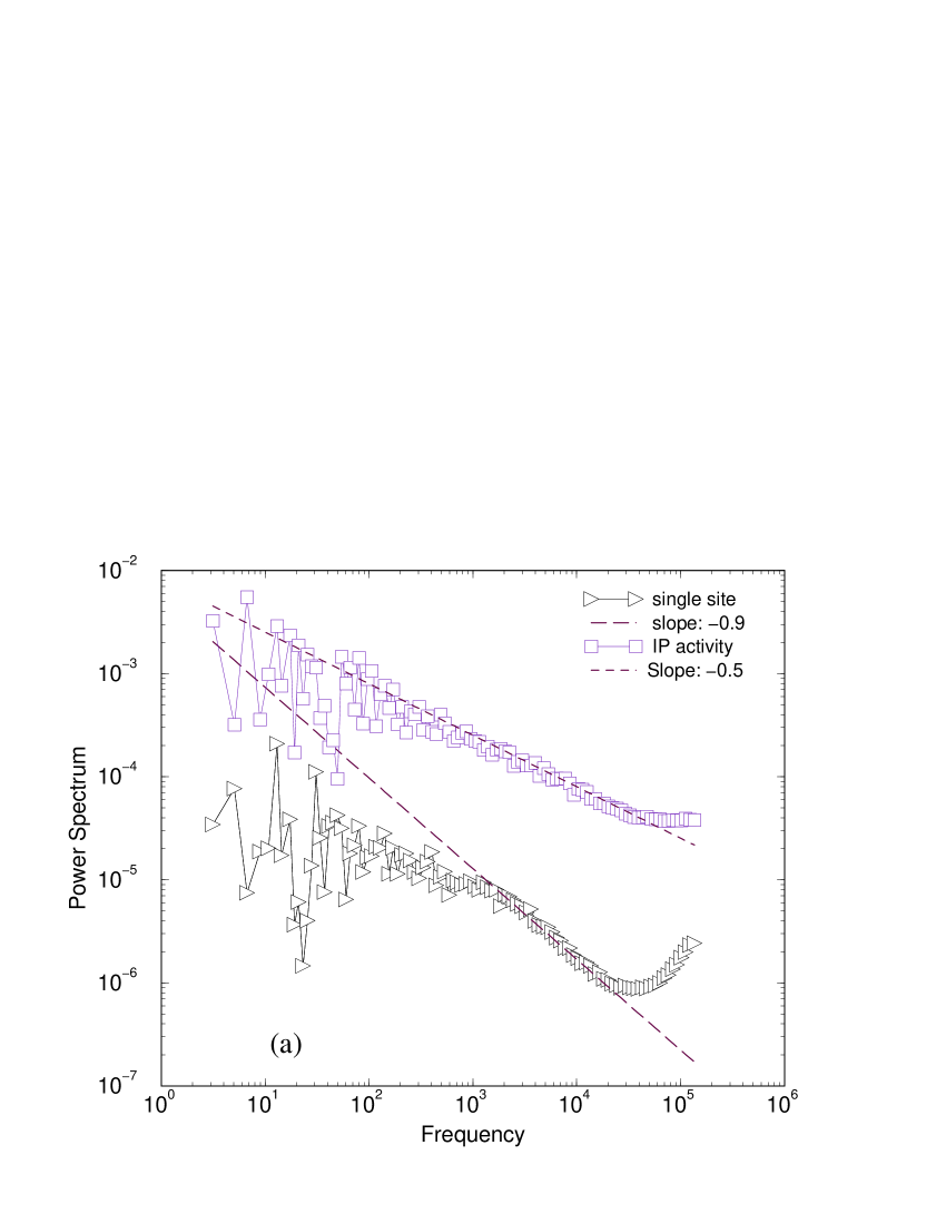
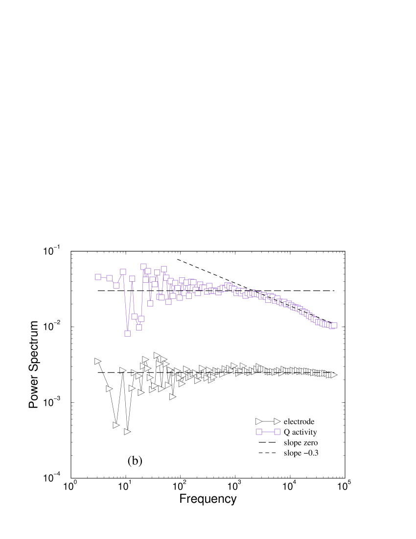
Figure 2: Power spectra of the recorded time series of activity at a single node (lower curves) and of a number of active nodes for transport of information packets (a) and tunneling electrons (b).

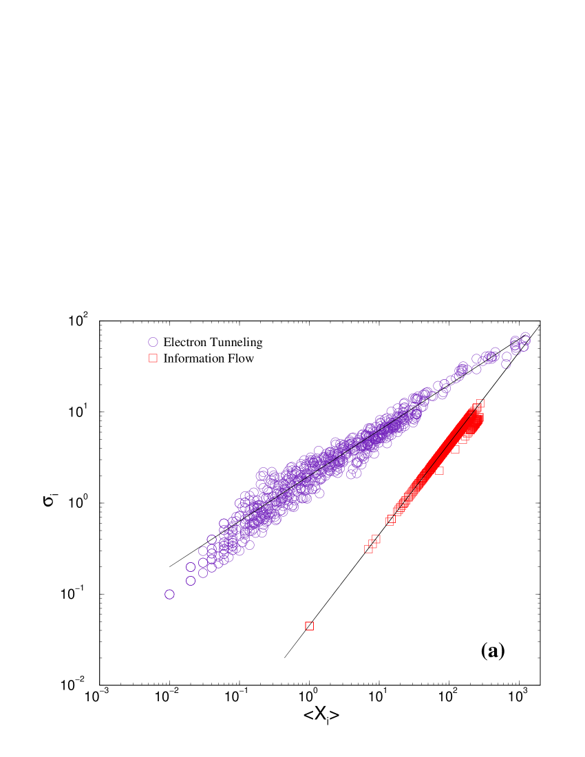
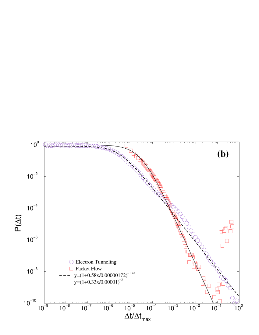
Figure 3: (a) Standard deviation $\sigma_{i}$ against average $<X_{i}>$ of the number of processing events at a node $i$ within time window $T_{win}=1000$ steps for the information packets and electron tunneling at cellular network in Fig. 1. Full lines indicate slopes $\mu=1/2$ and $\mu=1$. (b) Distributions of return-time intervals for the packet and electron transport. Fits are according to Eq. (5).

Multi-channel Noise. Monitoring the number of packets processed by each node within a fixed time window of $T_{win}=1000$ time steps, we make a set of time series $\{h_{i}(t_{w})\}$ for each node $i=1,2,\cdots N$, where $t_{w}=1,2,\cdots$ enumerates consecutive time windows. The computed standard deviation $\sigma_{i}$ of the time series $h_{i}(t_{w})$ for each node $i=1,2,\cdots N$ separately is shown against its average over all time windows $<X_{i}>\equiv<h_{i}(t_{w})>$ in Fig. 3 (a). It appears that the scaling law scaling_hsigma

$$\sigma_{i}\sim<X_{i}>^{\mu}\ ,$$ (4)

holds for all nodes, with the exponent $\mu=1$. With analogous analysis of the set of time series $\{Q_{i}(t_{w})\}$ and $<X_{i}>\equiv<Q_{i}(t_{w})>$ for the electron tunneling process at all nodes, we find that the scaling law (4) also holds, however, with clearly different exponent $\mu=1/2$, as shown in Fig. 3 (a).

Return-Times Statistics. In order to further substantiate the difference between the two transport processes, we determine the return-time statistics, which demonstrates how often the process occurs at a given node. The return time $\Delta t_{i}$ is defined as time interval between two consecutive events at a fixed node $i$. The distributions of return times appear to have power-law tails, that can be fitted with the $q$-exponential form Tsallis

$$P(\Delta t)=B_{q}\left[1-(1-q)\Delta t/\Delta t_{0}\right]^{1/(1-q)}\$$ (5)

with $q=1.58$ for the electron tunneling, and $q=1.33$ for the packet transport. The results are shown in Fig. 3 (b) for a reduced variable $\Delta t/\Delta t_{max}$, with $\Delta t_{max}$ is maximum observed interval for given process. This statistics suggests that longer waiting times and thus stronger correlations (larger $q>1$ values) occur more often in the electron tunneling. However, the corresponding noise fluctuations at individual nodes are compatible with $\mu=1/2$, contrary to the arguments given in Ref. scaling_hsigma .

In the packet processing, the local search is ineffective on the homogeneous (non-small world) network, and packets perform mostly random walk involving a large number of nodes (number of active nodes fluctuates around 94 for the density $\rho=100$). However, the packets interact due to queuing practically at all nodes along the path. The number of arriving packets at each node is limited to maximum three (number of links), whereas one packet is forwarded per time step. These transport constraints result in the noise fluctuations with the exponent $\mu=1$ on our planar graph.

V Role of Betweenness Centrality in Transport Processes

Contrary to the small-world graphs, in a homogeneous planar graph the even connectivity of nodes does not guarantee their even betweenness centrality. The betweenness centrality of nodes (links) in our network as shown in Fig. 1 appeares to be widely distributed. This topological inequality of nodes (links) is the basis for a different role that individual nodes (links) play in a dynamic process on that network. Additional difference developes due to microscopic details of the dynamics. Here we compare the topological betweenness centrality with dynamical flow for the two types of processes described above.

The computed topological betweenness centrality of nodes (links) of the network is also displayed in Fig. 1 via a color-code (exhibiting the spectrum from red, orange, yellow, green, blue, deep-blue and purple) for descending betweenness centrality in a suitably chosen log-binns. Note that, due to the constant node connectivity, the betweenness of links follows a similar pattern, so that nodes of high betweenness are placed along the links with high betweenness (shown with different widths of links in Fig. 1). The maximum-topological-flow spanning tree (shown in Fig. 1 right) connects pairs of nodes via the most frequent paths on the graph. Obviously, the skeleton of the tree represents the most frequent part of all paths on the graph. Nodes with largest centrality are placed along that path stretch.

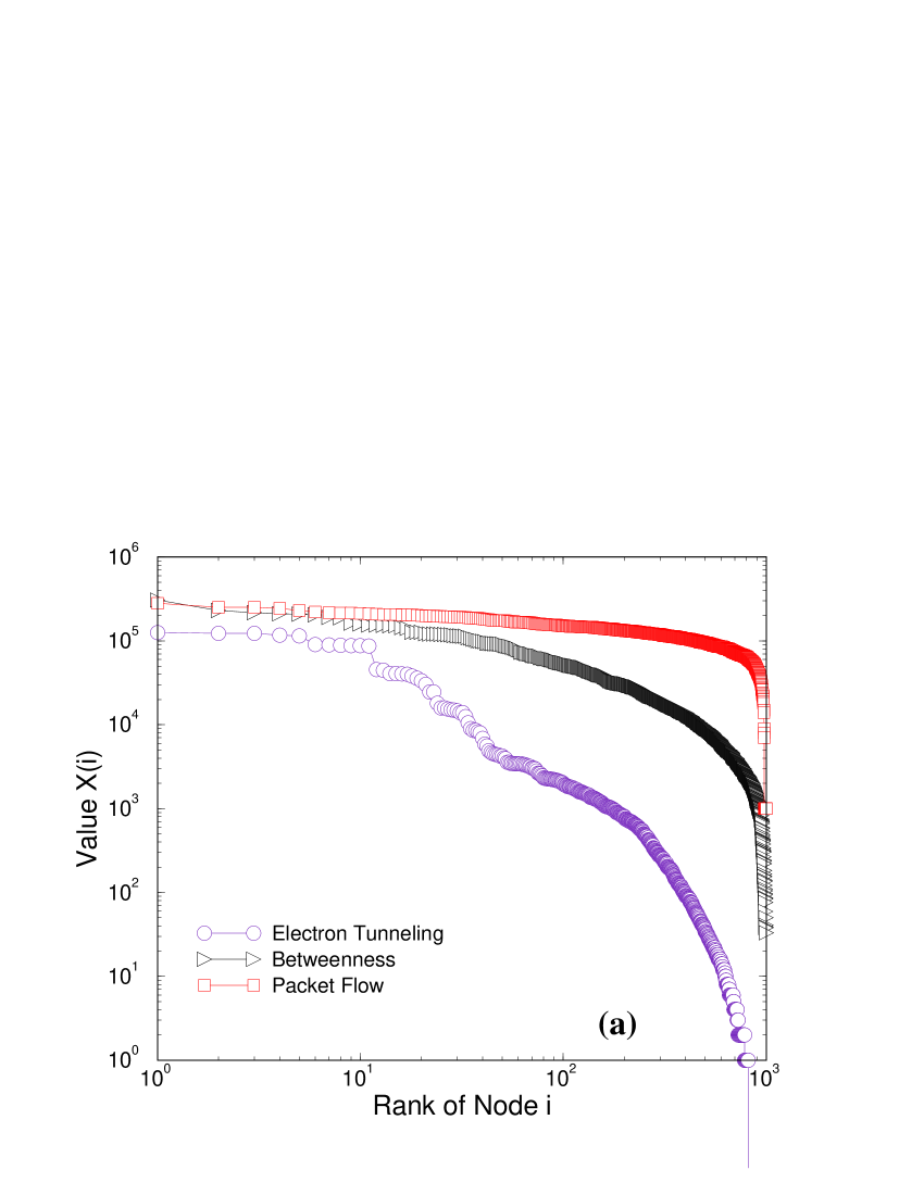
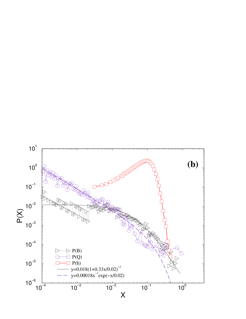
Figure 4: (a) Ranking statistics of nodes according to their topological betweenness centrality ($\triangleright$), dynamical number of tunnelings ($\bigcirc$) and number of processed packets ($\square$). (b) Distributions of topological centrality ($\triangleright$), number of tunnelings ($\bigcirc$), and number of processed packets ($\square$).

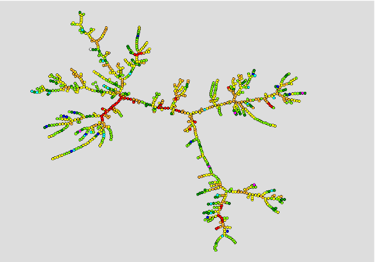
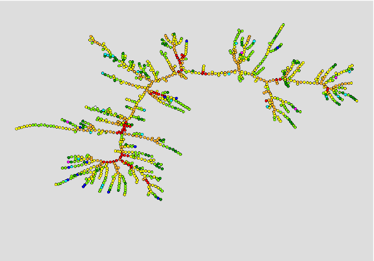
Figure 5: Information packets maximum-flow spanning tree (left) and tunneling-current maximum-flow spanning tree (right). Color-code represents topological betweenness of nodes, as in Fig. 1.

Additional details of the quantitative analysis are shown in Fig. 4. The inhomogeneous betweenness of nodes results in a broad ranking-statistics curve (stretched-exponential) and a broad distribution of betweenness (Fig. 4b). Compared to the topological betweenness, the dynamical betweenness (or flow), which is defined as number of packets processed by a node, in the case of packet transport appears to be more even in the node ranking statistics. The picture is compatible with the random walk dynamics, in which all nodes become almost equally busy in the transport process. This results in a narrow distribution of the dynamical information-flow betweenness, as shown in Fig. 4b. In the case of electron tunneling, the profile of the ranked dynamical betweenness of nodes is steeper, and consequently the distribution broader, compared to the topological betweenness. The reason is the directed flow of electrons between the electrodes, and additionally, the reduced active part of the graph, due to the selected position of the electrodes.

The difference between these two processes is also illustrated by their maximum-dynamic-flow spanning trees, which are shown in Fig. 5. Obviously, the two dynamic processes use the underlying graph topology in different ways. Nevertheless, the nodes with maximum topological betweenness are often placed along the central line on the dynamic flow trees, suggesting the key role of these nodes in both transport processes.

VI Conclusions

We have studied two dynamic processes on a homogeneous planar graph with scale-free loops in which we demonstrated several aspects of constraints in the network dynamics. First, the growth of the graph is constrained to a planar geometry and fixed node connectivity. This results in a non-small world graph, in which topological betweenness centrality of nodes (links) appears to be inhomogeneous, making the basis for nontrivial dynamical effects. Second, the graph’s geometry makes the constraints to the dynamic processes.

In the two types of diffusion processes—information packet flow and voltage-driven electron-tunneling—which take part between pairs of nodes on the graph, details of the dynamics result in different use of the underlying graph topology. The relevant features at microscopic scale are, on one side, random-walk dynamics with queuing of information packets, against directed transport of electrons with global constraint on the number of electrons at a node, on the other. In particular, we demonstrated the emergent quantitative difference in noise correlations, universal noise fluctuations and return-time statistics, and in the respective dynamical maximum-flow spanning trees. Our numerical data, for instance for the return-time distributions and the noise fluctuations, appear to be well fitted with theoretical expressions suggested in different concepts of the complex dynamical systems scaling_hsigma ; Tsallis . The full understanding of the occurrence of these laws in the transport on networks remains elusive. We hope that our numerical study may serve as a basis for further theoretical research to unravel the role of constraints in the dynamic processes on networks.

- (1) S. Boccaletti, V. Latora, Y. Moreno, M. Chavez, and D.-U. Hwang: Complex networks: Structure and dynamics, Physics Reports 424 (2006) 175-308
- (2) B. Tadić, G. J. Rodgers and S. Thurner, Transport on Complex Networks: Flow, Jamming, and Optimization, (submitted).
- (3) B. Tadić, S. Thurner, Physica A 332 (2004) 566-584; cond-mat/0307670
- (4) B. Tadić, T. Thurner, G.J. Rodgers, Phys. Rev. E 69 (2004) 036102
- (5) L.M. Pecora, M. Barahona, Chaos and Complexity Letters 1(1) (2005) 61-91
- (6) R. Guimera, A. Diaz-Guilera, F. Vega-Redondo, A. Cabrales, A. Arenas, Phys. Rev. Lett. 86 (2001) 3196-3199
- (7) L. Donetti, P.I. Hurtado, M.A. Muñoz, Phys. Rev. Lett. 95 (2005) 188701
- (8) K. Kaneko, On recursive production and evolvability of cells: Catalytic reaction network approach, in Geometric Structures of Phase Space in Multidimensional Chaos: Advances in Chemical Physics, Part B, edited by M. Toda et al., 103 (2005) 543-598
- (9) B. Tadić, S. Thurner, Physica A, 436 (2005) 183
- (10) M. Šuvakov and B. Tadić, Topology of Cell-Aggregated Planar Graphs, V.N. Alexandrov et al. Eds., Lecture Notes in Computer Science, Springer (Berlin) Part III, 3993 (2006) 1098-1105
- (11) B. Bollobás, Modern Graph Theory, Springer (New York) 1998.
- (12) B. Tadić, Modeling Traffic of Information Packets on Graphs with Complex Topology. P. Sloot et al. Eds., Lecture Notes in Computer Science, Springer (Berlin) Part I, 2657 (2003) 136-142
- (13) P. Moriarty, M.D.R. Taylor, M. Brust, Phys. Rev. Lett. 89 (2002) 248303
- (14) P. Moriarty, Pep. Prog. Phys. 64 (2001) 297-381
- (15) B.K. Ferry, S.M. Goodnick, Transport in Nanostructures, Cambridge University Press, 1997
- (16) R. Parthasarathy, X.M. Lin, H.M. Jaeger, Phys. Rev Lett. 87 (2001) 186807
- (17) S.C. Benjamin, Arxiv preprint cond-mat/0503319, 2005
- (18) M. Šuvakov and B. Tadić, Charge transport in cellular networks, in preparation.
- (19) M. Argolo de Menezes, A.L. Barabasi, Phys. Rev. Lett. 92 (2004) 028701
- (20) C. Tsallis, J. Stat. Phys. 52 (1988) 479