$G_{Q}$-corrections in Circuit Theory of Quantum Transport

Abstract

We develop a finite-element technique that allows one to evaluate correction of the order of $G_{Q}$ to various transport characteristics of arbitrary nanostructures. Common examples of such corrections are weak localization effect on conductance and universal conductance fluctuations. Our approach, however, is not restricted to conductance only. It allows in the same manner to evaluate corrections to noise characteristics, superconducting properties, strongly non-equilibrium transport and transmission distribution. To enable such functionality, we consider Green functions of arbitrary matrix structure. We derive a finite-element technique from Cooperon and Diffuson ladders for these Green’s functions. The derivation is supplemented with application examples. Those include transitions between ensembles and Aharonov-Bohm effect.

I Introduction

The theoretical predictions of weak localization WeakDiscovery and universal conductance fluctuations UCFDiscovery along with experimental discoveries in this direction GQExperimental ; bergman have laid a basis of modern understanding of quantum transport — transport in nanostructures — and have stimulated a considerable interest to the topic. Early studies mostly concentrated on diffusive electron transport. Both effects arise from quantum interference that is described in the language of slow modes: Cooperons and Diffusons.Rama ; Fukuyama Each mode of this kind brings a quantum (fluctuating) correction of the order of $G_{Q}\equiv e^{2}/\pi\hbar$ to the classical Drude conductance $G$ of the sample. This universal value sets an important division between classical conductors ($G\gg G_{Q}$) where interference effects are small and quantum ones ($G\simeq G_{Q}$) where the transport is essentially quantum.

A complementary approach to $G_{Q}$-corrections comes from Random Matrix Theory(RMT) of scattering Imry ; BeenakkerReview This approach relates statistical properties of scattering matrix of a nanostructure to those of a certain ensemble of random matrices. $G_{Q}$-corrections are understood in terms of fluctuations and rigidity of spectral density of these matrices. Although RMT approach can deal with diffusive systems, the most comprehensive setup includes the so-called quantum cavity — an element whose scattering matrix is presented by a completely random unitary matrix of a certain ensemble. The cavity can be seen as a region of space where electron motion is sufficiently chaotic (either ballistic or diffusive) and where electrons can get in and out through some constrictions cavity . The transport is determined by the propagation in the constrictions while random unitary matrix representing the cavity is responsible for ”randomization” of the scattering. The RMT approach does not necessary concentrate on the total conductance. One can work with transmission distribution: the averaged density of eigenvalues of transmission matrix squared. This transmission distribution appears to be useful in a much broader physical context: it determines not only conductance of nanostructures, but also noise, full counting statistics of charge transfers, and properties of the same nanostructure with superconducting leads attached BeenakkerReview ; NazarovOhm . It is a modern paradigm of quantum transport that an individual nanostructure is completely characterized by a set of transmission eigenvalues while transmission distribution describes the averaged properties of random nanostructures of the same design. This makes it relevant to study $G_{Q}$ corrections and fluctuations of transmission distribution Carlo-corrections ; Yuli-corrections . The density of transmission eigenvalues is of the order of $G/G_{Q}$, and $G_{Q}$ corrections are of the order of $\delta G/G_{Q}\simeq 1$.

The microscopic Cooperon-Diffuson description is equivalent to a proper RMT approach. This is best illustrated in the framework of more general supersymmetric theory Efetov that allows for non-perturbative treatment of fluctuations in quantum scattering. The Cooperons and Diffusons in this theory are fluctuations of supersymmetric field around the saddle point. For quantum cavity, only a single mode of these fluctuations is relevant. The integration over these modes reproduces RMT results Efetov ; Zirnbauer ; Iida .

One can describe nanostructures in the framework of a simple finite-element approach usually termed ”circuit theory”. The circuit theory has originated from attempts to find simple solutions of Usadel equations in superconducting heterostructures circuit-theory-old . However, it has been quickly understood that theories of the same structure can be useful in much broader context: one can compute transmission distribution NazarovOhm ; ct-yuli , noise and counting statistics fcs-yuli , investigate spin effects spin and non-equilibrium phenomenanon-eq . In circuit theory, a nanostructure is presented in a language similar to that of electric circuits: It consists of nodes, reservoirs and connectors. A node is in fact a quantum cavity, a connector can be of very different types: tunnel junction, ballistic contact and diffusive wire and is generally characterized by a set of transmission coefficients. In circuit theory, each node is described by a matrix related to the electron Green’s function. In the limit $G\gg G_{Q}$ the circuit theory provides a set of algebraic equations that allow one to express the matrices in the nodes in terms of fixed matrices in the reservoirs.

In this article, we present a technique to evaluate $G_{Q}$-corrections for arbitrary nanostructures described by circuit theory. To allow for various applications, we consider $G_{Q}$ corrections to multi-component Green’s functions of arbitrary matrix structure. We are able to present $G_{Q}$ corrections in a form of a determinant made of derivatives of Green’s functions in the nodes with respect to self-energy parts. In terms of a supersymmetric sigma-model, this corresponds to expansion of the action up to quadratic terms. However, the formulation we present does not contain any anti-commuting variables that complicate applications of sigma-models. The determinant is just that of a finite matrix, this facilitates the computation of $G_{Q}$ corrections for nanostructures of complicated design.

The structure of the article is as follows. To make it self-contained, we start with a short outline of circuit theory of multi-component Green’s functions adjusted for the purposes of further derivations. In Section III we derive microscopic expressions for $G_{Q}$ corrections and specify to finite-elements in Section IV. Next Section V is devoted to description of spin-orbit scattering and magnetic-field de-coherence that are used to describe transitions between different RMT ensembles. Since Aharonov-Bohm effect plays an important role in experimental observation of $G_{Q}$ corrections, we explain how to incorporate it to our scheme in a short separate section VI. We illustrate the technique with several examples (Section VII) concentrating on a simplest $2\times 2$ matrix structure that suits to calculate $G_{Q}$ corrections to transmission distribution. The examples also involve simplest circuits: One with a single node and two arbitrary connectors, a chain of tunnel junctions, and two-node four-junction circuit to demonstrate Aharonov-Bohm effect. We summarize in Section VIII.

II From Green’s functions to finite elements

In this article, we consider Green’s functions of arbitrary additional matrix structure with $N_{ch}$ indices. We do this for the sake of generality: This allows for description of super-conductivity, incorporating Keldysh formalism and treating non-equilibrium and time-dependent problems. This is also extremely convenient, since the most relations in use do not depend on the ”physical meaning” of the structure. We use ”hat” symbol for operators in coordinate space and ”check” symbol for matrices in additional indices. The Green’s function thus reads: $\hat{G}\equiv\check{G}(\bm{x},\bm{x}^{\prime})$, $\bm{x}$ stands for (three-dimensional) coordinate. The general Green’s function is defined as the solution of the following equation

$$\left[-\check{\Sigma}(\bm{x})-\hat{H}\right]\check{G}(\bm{x},\bm{x}^{\prime})=\delta(\bm{x}-\bm{x}^{\prime}).$$ (1)

All physical quantities of interest can be in principle calculated from Green’s functions. We address here the quantum transport of electrons in disordered media. In this case, one can work with common Hamiltonian

$$\hat{H}=\hat{H}_{0}+u(\bm{x}),\,\,\,\hat{H}_{0}=-\frac{1}{2m}\nabla^{2}_{\bm{x}}+U(\bm{x}).$$ (2)

Here $U(\bm{x})$ describes the design of nanostructure: Potential ”walls” that determine its shape, and form ballistic quantum point contacts, potential barriers in tunnel junctions, etc. The potential $u(\bm{x})$ is random: it describes the random impurity potential responsible for diffusive motion of electrons, isotropization of electron distribution function and, most importantly for this article, fluctuations of transport properties of the nanostructure. The physics at space scales exceeding the isotropization length (which is the mean free path in the case of diffusive transport) does not depend on a concrete model of randomness of this potential. Most convenient and widely used model assumes normal distribution of $u(\bm{x})$ characterized by the correlator $\langle u(\bm{x})u(\bm{x}^{\prime})\rangle=w\delta(\bm{x}-\bm{x}^{\prime})$. It is important for us that both $\hat{H}_{0}$ and $u(\bm{x})$ are diagonal in check indices.

Most evident choice of self-energy matrix is $\check{\Sigma}(\bm{x})=-\epsilon$, $\epsilon$ being energy parameter of the Green’s function. $\check{\Sigma}$ is more complicated in the theory of superconductivity. We will find it convenient, at least for derivation purposes, to work with arbitrary $\check{\Sigma}(\bm{x})$. We can also consider more general situation with non-local $\check{\Sigma}(\bm{x},\bm{x^{\prime}})$.

Provided the conductance of the nanostructure is sufficiently high ($G\gg G_{Q}$), one can disregard quantum $G_{Q}$-corrections and work with semiclassical averaged Green’s functions. Closed equations for those are obtained with the non-crossing approximation AGD . They include the impurity self-energy,

$$\left[-\check{\Sigma}(\bm{x})-\check{\Sigma}_{imp}-\hat{H}_{0}\right]\check{G}(\epsilon;\bm{x},\bm{x}^{\prime})=\delta(\bm{x}-\bm{x}^{\prime}),$$ (3)

$$\check{\Sigma}_{imp}(\bm{x})=w\check{G}(\bm{x},\bm{x})$$ (4)

At space scales exceeding the mean free path, one can write closed equations for the Green’s function in the coinciding points Usadel ; Larkin . It is convenient to change notations introducing dimensionless $\check{G}(\bm{x})\rightarrow G(\bm{x},\bm{x})/i\pi\nu$, with $\nu$ the density of states at Fermi energy. For purely diffusive transport, one obtains Usadel equation

$$\nabla\cdot\check{\bm{j}}-i\pi\nu[\check{\Sigma}(\bm{x}),\check{G}(\bm{x})]=0,\ \ \ \ \check{\bm{j}}=-\pi D(\bm{x})\nu\check{G}\bm{\nabla}\check{G},$$ (5)

$D$ being the diffusion coefficient. The solutions of Usadel equations are defined only if one takes into account boundary conditions at ”infinity”: Equilibrium Green’s functions in the macroscopic leads adjacent to the nanostructure. It turns out that $\check{G}$ satisfies unity condition $\check{G}^{2}=\check{1}$. For situations where the transport is not entirely diffusive, one would supplement the Usadel equation with boundary conditions of various kinds (c.f. Kuprianov ).

An alternative way to proceed is to notice that the Usadel equation is almost a conservation law for the matrix current $\check{\bm{j}}$, which allows for a finite element approach. This conservation law is exact at space scale smaller than the coherence length estimated as $\sqrt{D\Sigma}$. It does not relay on assumption of diffusivity: It occurs because the Hamiltonian $\hat{H}$ commutes with the ”check” structure. It is then natural to proceed to the separation of the nanostructure into regions where $\check{G}(\bm{x})$ can be assumed constant. The next steps are the same as in traditional circuit theory of electric circuits, which exploits conservation of electric current and finite discretization of the system onto regions of approximately constant voltage — nodes. Each node is connected by connectors to other nodes or reservoirs, those representing macroscopic leads.

After the discretization of the nanostructure we can write a Kirchhoff-like equation

$$\sum_{c}\check{I}_{c}+\sum_{\alpha}\check{I}_{l,\alpha}=0,$$ (6)

where the indices $c$ and $\alpha$ label the nodes and the connectors of the nanostructure. The current through a connector $c$ which connects nodes $c1$ and $c2$ reads

$$\check{I_{c}}=\frac{1}{4}\sum_{n}\frac{T^{c}_{n}[\check{G}_{c1},\check{G}_{c2}]}{1+T^{c}_{n}(\check{G}_{c1}\check{G}_{c2}+\check{G}_{c2}\check{G}_{c1}-2)/4},$$ (7)

$\{T^{c}_{n}\}$ being the set of transmission eigenvalues of the transmission matrix squared relative to the connector. Eq. 5 shows that the current $\check{\bm{j}}$ is not fully conserved; to this aim we included in Eq. 6 a leakage current

$$\check{I}_{l,\alpha}=-\frac{i\pi}{\delta_{\alpha}}[\check{\Sigma}_{\alpha},\check{G}_{\alpha}],\ \ \ \ \ \ \delta_{\alpha}=\frac{1}{\nu V_{\alpha}},$$ (8)

where $V_{\alpha}$ is the volume of the node; $\delta_{\alpha}$ can be easily recognized as the average level spacing in the node.

It is opportune to notice that the conservation law (6) can be obtained by requiring that the values assumed by the matrix Green’s function in the nodes are such to minimize the following the action

$${\cal S}=\sum_{c}{\cal S}_{c}+\sum_{\alpha}{\cal S}_{\alpha}$$ (9)

$${\cal S}_{c}=\frac{1}{2}\sum_{n}\mbox{Tr}\ln\left[1+\frac{T_{n}}{4}(\check{G}_{c1}\check{G}_{c2}+\check{G}_{c2}\check{G}_{c1}-2)\right]$$ (10)

$${\cal S}_{\alpha}=-\frac{i\pi}{\delta_{\alpha}}\mbox{Tr}\check{\Sigma}_{\alpha}\check{G}_{\alpha}.$$ (11)

The minimization of the action must be carried out provided that the Green’s functions in each node satisfy the normalization condition $\check{G}_{\alpha}^{2}=1$; this implies that the variation of the Green’s function $\delta\check{G}_{\alpha}$ has to anti-commute with $\check{G}_{\alpha}$ itself. A possible way to satisfy this condition is to write the variation as

$$\delta\check{G}_{\alpha}=\check{G}_{\alpha}\delta\check{v}_{\alpha}-\delta\check{v}_{\alpha}\check{G}_{\alpha},$$ (12)

where no restriction is imposed on $\delta\check{v}_{\alpha}$. The Kirchhoff equations are then re-written as

$$\frac{\delta\cal{S}}{\delta\check{v}_{\alpha}}=[\check{G},\frac{\delta\cal{S}}{\delta\check{G}_{\alpha}}]=0.$$ (13)

The same action can be used at microscopic level too, even before averaging over $u(\bm{x})$. To do this, we note once again that $\check{\Sigma}(\bm{x})$ form , at least formally, a set of parameters of our model. This can be straightforwardly extended to non-local operators $\Sigma(\bm{x},\bm{x}^{\prime})$. To this end, we define the action in terms of the following variational formula

$$\delta{\cal S}=-\int d\bm{x}d\bm{x^{\prime}}{\rm Tr}\left[\check{G}(\bm{x}^{\prime},\bm{x})\delta\check{\Sigma}(\bm{x},\bm{x}^{\prime})\right],$$ (14)

which is traditional in Green’s function applicationsAGD ; Luttinger . With making use of formal operator traces, this action can be written in terms of either $\hat{\Sigma}$ or $\hat{G}$,

$${\cal S}={\rm Tr}\ln\left(\hat{\Sigma}+\hat{H}\right);$$ (15)

$${\cal S}={\rm Tr}\left[-\ln\left(-\hat{G}\right)-(\hat{\Sigma}+\hat{H})\hat{G}\right];$$ (16)

apart from a constant. Eq. 1 is reproduced by varying either (15) or (16) over $\hat{\Sigma}$ or $\hat{G}$ respectively. Since we are not planning to treat $G_{Q}$ corrections beyond perturbation theory, we do not attempt to use the exponent of this action as an integrand in some path integral representation of a result of exact averaging over $u(\bm{x})$. This has been done in Efetov for supersymmetric matrices $\check{Q}$ and in Larkin-great for Keldysh-based two-energy matrices $\check{Q}(\bm{x},\epsilon,\epsilon^{\prime})$. We note, however, that the action used in Efetov ; Larkin-great is equivalent to (9) if one substitutes $\check{G}=\check{Q}$.

To this end, for averaged Green’s functions the action in use is defined simply as

$$\delta{\cal S}=-\int d\bm{x}d\bm{x^{\prime}}{\rm Tr}\left[<\check{G}(\bm{x}^{\prime},\bm{x})>\delta\check{\Sigma}(\bm{x},\bm{x}^{\prime})\right].$$ (17)

III $G_{Q}$-corrections to multi-component Green’s functions

In this Section, we outline a microscopic approach to $G_{Q}$ corrections suitable for multi-component Green’s functions. The main idea is the same as in Yuli-corrections ; Yuli-Annalen where similar derivation has been done for purely diffusive case and for a concrete $2\times 2$ matrix structure. It is known Rama ; Fukuyama that diffuson and cooperon modes responsible for $G_{Q}$ corrections are presented as ladder diagrams made from averaged Green’s functions. In usual technique, such diagrams have vertices corresponding to two current operators in Kubo formula. One does not have to work with vertices: Instead, one considers Cooperon and Diffuson contributions to the action that do not have any. The part of the action that presents $G_{Q}$ corrections is given by wheel diagrams. These wheels are made of either Cooperon or Diffuson ladder sections in a straightforward way (see Fig. 1)

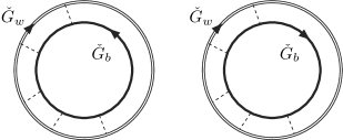
Figure 1: Wheel diagrams that determine $G_{Q}$-corrections to the action. Single (double) line represents the Green’s functions from the black (white ) block while dashed lines represent the averaging over disorder. The Diffuson (left) and Cooperon (right) wheel differ by mutual orientation of the lines.

We argue that the optimal way to present this part of the action is to double the existing ”check” structure and to consider Eq. 1 in so-extended setup. Indeed, suppose we would like to address the most general application of $G_{Q}$ corrections: Parametric correlations parametric . In this case, we start with two different ”worlds” corresponding to two different sets of parameters. In our case, all parameters can be in principle incorporated into $\check{\Sigma}(\bm{x})$. So we have ”white” and ”black” sets, $\check{\Sigma}_{b},\check{\Sigma}_{w}$, those define corresponding non-averaged Green’s functions $\check{G}_{b},\check{G}_{w}$. The averaging over the random potential $u({\bm{x}})$ provides correlations between the two ”worlds” and gives the rungs of the ladder diagrams that involve ”white” and ”black” Green’s functions (Fig. 1). This is to obtain the Diffuson ladder wheel. The Cooperon ladder wheel is obtained by inverting the direction of the Green’s function in one of the ”worlds”. This corresponds to using transposed self-energies for this world, $\check{\Sigma}_{w}\rightarrow(\check{\Sigma}_{w})^{T}$. This guarantees that the corresponding Green’s functions are also transposed. Fluctuations at the same values of the parameters are naturally given by diagrams where $\check{\Sigma}_{b}$ and $\check{\Sigma}_{w}$ either are the same in both ”worlds” (Diffusons), or mutually transposed (Cooperons).

Finally, we note that the doubled structure is also useful for evaluation of the weak localization correction. In this case, the last section of the Cooperon ladder is twisted before closing the wheel.

To proceed further, let us introduce the operators $\hat{K}$ presenting a section of a corresponding ladder,

$$\hat{K}_{\rm diff}^{ab,cd}(\bm{x},\bm{x^{\prime}})=w(\bm{x})\langle G_{b}^{ac}(\bm{x},\bm{x}^{\prime})\rangle\langle G_{w}^{db}(\bm{x^{\prime}},\bm{x})\rangle$$ (18)

$$\hat{K}_{\rm cooper}^{ab,cd}(\bm{x},\bm{x}^{\prime})=w(\bm{x})\langle G_{b}^{ac}(\bm{x},\bm{x}^{\prime})\rangle\langle G_{w}^{bd}(\bm{x},\bm{x}^{\prime})\rangle$$ (19)

where Latin letters represent ”check” indices. As we have noted, the ”white” Green’s function is transposed for the Cooperon. Those are operators in the space spanned by the coordinates and the two check indices.

Summing up all diagrams, we find the formal operator expressions for contributions to the action. For fluctuations, we have

$${\cal S}_{G_{Q}}={\rm Tr}\left[\ln(1-\hat{K}_{\rm cooper})\right]+{\rm Tr}\left[\ln(1-\hat{K}_{\rm diff})\right]$$ (20)

diffuson and cooperon contributions are given by $\hat{K}_{diff}$, $\hat{K}_{cooper}$ respectively. For weak localization correction, one has to account for the fact that the last ladder section is twisted. We do this by introducing the permutation operator $\check{P}$, which exchange ”check” indices,

$$\hat{P}\,\hat{K}^{ab,cd}=\hat{K}^{ba,cd}.$$ (21)

The contribution to the action becomes

$${\cal S}_{wl}=\frac{1}{2}{\rm Tr}\left[\hat{P}\ln(1-\hat{K}_{\rm cooper})\right].$$ (22)

The factor one half is included in the last formula to take into account that ”black” and ”white” Green’s functions, in the case of weak localization, are not anymore independent. We note that $\hat{K}$ for the Cooperon is symmetric with respect to index exchange, so that $\hat{K}$ and $\hat{P}$ commute. The eigenfunctions and the eigenvalues of $K$ are therefore either symmetric ($K^{+}$) or anti-symmetric ($K^{-}$) with respect to permutations. We can rewrite the last expression as a sum over these eigenvalues

$${\cal S}_{wl}=\frac{1}{2}\sum_{n}\left[\ln(1-K^{+}_{n})-\ln(1-K^{-}_{n})\right].$$ (23)

It is clear from the previous discussion that, in order to calculate the $G_{Q}$ corrections, one has to evaluate the eigenvalues of the ladder section $\check{K}$, both for Cooperon and Diffuson. We introduce now a method to compute this matrix easily. The observation is that the ladders under consideration are not specific for $G_{Q}$-corrections: The same ladders determine a response of semiclassical Green’s functions upon variation of $\check{\Sigma}$ remark .

To see this, let us go back to non-averaged Green’s functions. We keep in mind that we have doubled the ”check” space to include white and black sector. We add by hand a source term: The self-energy which mixes up ”black” and ”white” Green’s functions, $\delta\check{\Sigma}_{bw}(\bm{x})$. This source term will give rise to a correction to the Green’s function in the same black-white sector. In the first order, we have

$$\delta\check{G}_{bw}(\bm{x},\bm{x}^{\prime})=\\ -\int d\bm{x}_{1}d\bm{x}_{2}\check{G}_{b}(\bm{x},\bm{x}_{1})\delta\check{\Sigma}_{bw}(\bm{x}_{1},\bm{x}_{2})\check{G}_{w}(\bm{x}_{1},\bm{x}^{\prime}),$$ (24)

which is best illustrated by the diagram in Figure 2. Next step is to include the effect of the random potential $u(\bm{x})$. We average Eq. 24 limiting ourselves to the non-crossing approximation and obtaining a set of ladder diagrams (Fig. 2.) By summing up all the contributions we obtain the correction—taken in coinciding points—to the Green’s function

$$\langle\delta\check{G}_{bw}(\bm{x},\bm{x})\rangle=\frac{1}{w(\bm{x})}\frac{\hat{K}_{\rm diff}}{1-\hat{K}_{\rm diff}}\delta\check{\Sigma}_{bw}\,(\bm{x}).$$ (25)

Eq. (25) is very valuable: it demonstrates that the response of the Green’s function to the source term $\delta\check{\Sigma}_{bw}$ is determined by the same ladder operator $\hat{K}$, which we need to compute $G_{Q}$ corrections.

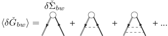
Figure 2: The response of Green’s function $\delta\check{G}_{bw}$ on self-energy $\check{\Sigma}_{bw}$ in semiclassical non-crossing approximation is determined by the sum of ladder diagrams. This allows to express the wheel diagrams in terms of eigenvalues of response kernels.

At the space scale of isotropization length $\hat{K}\sim 1$. Usually one is interested in the contribution arising from the larger space scale where Cooperon-Diffuson approximation is valid. At this scale, the eigenvalues of $\hat{K}$ are either zero or very close to one. To see this, we cite the results for the homogeneous case with $\check{\Sigma}={\rm const}(\bm{x})$. A convenient basis in ”check” space is one where $\check{\Sigma}$ is diagonal, the eigenvalues being $\Sigma_{n}$. The Green’s function is diagonal in this basis as well, $G_{n}=s_{a}\equiv\rm{sign\ Im}(\Sigma_{a})$. Owing to homogeneity, the section operator is diagonal in the wave vector representation, its eigenvalues being $K^{nm}(\bm{q})$. Direct calculation similar to Fukuyama gives $K^{nm}(\bm{q})=0$ if $s_{n}=s_{m}$. If $s_{n}\neq s_{m}$,

$$1-K^{ab}(\bm{q})\approx\tau\left(is_{b}(\Sigma_{a}-\Sigma_{b})+D\bm{q}^{2}\right)+...$$ (26)

for $\Sigma\tau,ql\ll 1$($\tau=2\pi w\nu$ is the isotropization time). This equation makes the relation between our technique and the common technique for Cooperons and Diffusons in homogeneous media. Usually, the self-energy $\Sigma$ has equal number of eigenvalues with positive and negative imaginary parts. In this case, at each $\bm{q}$, $\hat{K}$ has $N_{ch}^{2}/2$ zero and $N_{ch}^{2}/2$ non-zero eigenvalues.

Now we note that zero eigenvalues contribute neither to (20) nor to (25). As to those close to $1$, we may replace $\hat{K}$ by $1$ in the numerator of (25). We also note that $\delta\check{G}$ can be presented as the derivative of the action (c.f. Eq. 14). Therefore, we can write the $G_{Q}$ corrections due to the diffuson modes to the action in terms of a determinant made of derivatives of the semiclassical action with respect to $\check{\Sigma}_{bw},\check{\Sigma}_{wb}$

$${\cal S}_{G_{Q},{\rm diff}}=-\ln\det{{}^{\prime}}\left(-w(\bm{x})\frac{\delta^{2}{\cal S}}{\delta\check{\Sigma}_{wb}\delta\check{\Sigma}_{bw}}\right).$$ (27)

The ”prime” sign of the determinant signals that the zero eigenvalues shall be excluded: $det^{\prime}$ is defined as the product of all non-zero eigenvalues. Indeed, as we have seen, some variations of self-energies do not change the Green’s functions giving rise to zero eigenvalues. We also note that the $G_{Q}$ corrections are not affected by the concrete form of $w(\bm{x})$: Since the determinant of matrix product is a product of their determinants, this matrix gives a constant contribution to the action which does not affect any physical quantities.

IV Method

Let us now adapt the microscopic relation (27) to the finite-element approach outlined in the Section II.

With all previous derivations, this step is easy. We just replace the actual $\bm{x}$-dependent $\check{G}$ and $\check{\Sigma}$ by constants in each node. To get the action in these terms, one integrates over the volume of each node so that the formula (14) reads

$$\delta{\cal S}=-\sum_{\alpha}\frac{i\pi}{\delta_{\alpha}}{\rm Tr}\left[\check{G}_{\alpha}\delta\check{\Sigma}_{\alpha}\right],$$ (28)

where the summation is over the nodes. The discrete analog of the determinant relation (27) is now

$${\cal S}_{G_{Q},{\rm diff}}=-\ln\det{{}^{\prime}}\left(-\frac{w_{\alpha}}{V_{\alpha}}\frac{\delta^{2}{\cal S}}{\delta\check{\Sigma}_{wb}\delta\check{\Sigma}_{bw}}\right)\\ -\ln\det{{}^{\prime}}\left(\frac{\pi}{2\tau_{\alpha}\delta_{\alpha}}\frac{\delta^{2}{\cal S}}{\delta\check{\eta}_{wb}\delta\check{\eta}_{bw}}\right)={\rm const}-\ln\det{{}^{\prime}}\left(\frac{\delta^{2}{\cal S}}{\delta\check{\eta}_{wb}\delta\check{\eta}_{bw}}\right)$$ (29)

where we have introduced dimensionless response matrix $\check{\eta}_{\alpha}\equiv i\pi\Sigma/\delta_{\alpha}$ and noticed that the matrix $\propto w$ brings a constant contribution to the action. The response matrix is determined from the solution of the Kirchhoff equations at vanishing source term $\check{\eta}_{\alpha}^{bw}$. It has $N_{nodes}\cdot N_{ch}^{2}/2$ non-zero eigenvalues and the same number of zero ones. We observe that at $\Sigma_{w,b}=0$ the eigenvalues of this matrix do not depend on the volume of the nodes, they are determined by the transmission eigenvalues of the connectors only, and are of the order of $G/G_{Q}$. Since rescaling of all conductances gives only an irrelevant constant contribution to the action, the $G_{Q}$ corrections depend only on the ratios of conductances of the connectors: This manifests the universality of these corrections.

The circuit theory action (9)is given in terms of $\check{G}_{\alpha}$. It is advantageous to present the answer for ${\cal S}_{G_{Q}}$ in terms of the expansion coefficients of the action around the saddle-point: The solution of semiclassical circuit-theory equations. That is, to use $\delta^{2}{\cal S}/{\delta\check{G}_{wb}\delta\check{G}_{bw}}$ instead ${\delta^{2}{\cal S}}/{\delta\check{\eta}_{wb}\delta\check{\eta}_{bw}}$. If the latter matrix were invertible, we would make use of the fact that $\delta^{2}{\cal S}/{\delta\check{G}_{wb}\delta\check{G}_{bw}}=({\delta^{2}{\cal S}}/{\delta\check{\eta}_{wb}\delta\check{\eta}_{bw}})^{-1}$. In fact, owing to the constrain $\check{G}^{2}=1$, there is a big number of zero eigenvalues in the response matrix. So the task in hand is not completely trivial.

We proceed as follows. We expand the action by replacing each $\check{G}$ in each node by

$$\check{G}=\check{G}_{0}+\check{g}-\check{G}_{0}\check{g}^{2}/2+...$$ (30)

and collecting terms of the second order in $\check{g},\check{\eta}$. The form (30) satisfies the constrain $\check{G}^{2}=1$ up to second order terms provided $\check{g}\check{G}_{0}+\check{G}_{0}\check{g}=0$. Let us work in the $N_{ch}^{2}N_{node}$-dimensional space indexed with the ”bar” index $\bar{a}$ composed of two ”check” indices and one node index, $\bar{a}\equiv(a,b,\alpha)$. We present the result of the expansion as

$$\delta{\cal S}=g^{wb}_{\bar{a}}M_{\bar{a}\bar{b}}g^{bw}_{\bar{b}}-\eta_{\bar{a}}g^{bw}_{\bar{a}}.$$ (31)

The variation of (31) under the constrain $\check{g}\check{G}_{0}+\check{G}_{0}\check{g}=0$ gives the response matrix $\delta^{2}{\cal S}/\delta\eta_{\bar{a}}\delta\eta_{\bar{a}}$. Next we consider matrix $\Pi_{\bar{a}\bar{b}}$ defined trough the following relation:

$$\Pi_{\bar{a}\bar{b}}g^{bw}_{\bar{b}}\rightarrow$$

$$\frac{1}{2}\left(\check{g}-\check{G}_{0}\check{g}\check{G}_{0}\right)\rightarrow$$

$$\frac{1}{2}\left(\check{g}^{bw}-\check{G}_{b}\check{g}^{bw}\check{G}_{w}\right),$$ (32)

the last equation makes white-black block separation explicit. We note that $\Pi_{\bar{a}\bar{b}}$ is a projector: It separates ”bar” space on two subspaces where $\check{g}$ either commutes or anti-commutes with $\check{G}_{0}$, and projects an arbitrary $\check{g}$ onto anti-commuting subspace. Applying this projector to Eq. 31, we show that the projected matrix $\Pi_{\bar{a}\bar{b}}M_{\bar{b}\bar{c}}\Pi_{\bar{c}\bar{b}}$ is an inverse of the response matrix within the anti-commuting subspace.

$${\cal S}_{G_{Q}}=\ln{\rm det}^{\prime}\left(\Pi_{\bar{a}\bar{b}}M_{\bar{b}\bar{c}}\Pi_{\bar{c}\bar{b}})\right)=$$

$$\ln{\rm det}\left(\Pi_{\bar{a}\bar{b}}M_{\bar{b}\bar{c}}\Pi_{\bar{c}\bar{b}}+\delta_{\bar{a}\bar{b}}-\Pi_{\bar{a}\bar{b}}\right)$$ (33)

In the last equation we add the matrix $1-\hat{\Pi}$. This procedure replaces all zero eigenvalues with $1$, so one can evaluate a usual determinant.

We remind that as far as fluctuations are concerned, there are two contributions of this kind coming from Diffuson and Cooperon ladder respectively. The weak localization correction involves permutation operator that sorts out eigenvalues involved according to (23). With this, the equations (33) and (29) give the $G_{Q}$ corrections in an arbitrary circuit-theory setup in the most general form.

V Decoherence and Ensembles

Until now we have assumed that the Hamiltonian commutes with the ”check” structure and is invariant with respect to time reversal. This implies strict coherence of waves with different ”check” index which propagate in the disordered media described by this Hamiltonian. Even small ”check”-dependent perturbations of the symmetric Hamiltonian give accumulating phase-shifts to these waves and may significantly change their interference patterns at long distances. Due to its random nature, such phase-shifts can be regarded as decoherence although this should not be confused with a real decoherence coming from interaction-driven inelastic processes altrev2 .

In real experimental situations, two sources of such decoherence are usually of importance: spin-orbit scattering and magnetic field. Already early studies of $G_{Q}$ corrections WeakDiscovery ; bergman have revealed their significant dependence on these two factors in the regime where those are too weak to affect the semiclassical transport. From the RMT point of view, these factors, upon increasing their strength, provide transitions form orthogonal ensemble (symmetric Hamiltonian) to two different ensembles: symplectic (spin-orbit interaction) and unitary (magnetic field) Efetov .

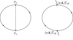
Figure 3: Second-order diagrams in spin-orbit interaction (left) and magnetic field (right) provide decoherence terms in the action. These terms describe transitions between pure RMT ensembles.

We show in this Section how to incorporate spin-orbit scattering and magnetic field into our scheme. The most convenient way is to present them as perturbative corrections to $\check{G}$-dependent action (Fig. 3.)

The spin-orbit scattering enters the Hamiltonian in the form $\hat{H}_{so}=\check{\sigma}_{a}H^{a}(\bm{x},\bm{x^{\prime}})$, $H^{a}(\bm{x},\bm{x^{\prime}})=-H^{a}(\bm{x^{\prime}},\bm{x})$, $\check{\sigma}_{a}$ representing spin Pauli matrices in ”check” space. In the second order in $H^{a}$ the averaging gives (Fig. 3)

$${\cal S}_{so}=\int d{\bm{x}}\frac{\pi\nu}{8\tau_{so}(\bm{x})}{\rm Tr}\left[\check{G}(\bm{x})\check{\sigma}_{a}\check{G}(\bm{x})\check{\sigma}_{a}\right]$$ (34)

At the level of microscopic approach, the spin-orbit scattering takes place anywhere in the nanostructure. In the finite-element approach, it is advantageous to ascribe spin-orbit scattering to nodes rather than to connectors. This is consistent with the main idea of our scheme: Random phase-shifts take place in the nodes. The spin-orbit contribution in each node $\alpha$ is obtained by integrating (34) over the node,

$${\cal S}_{so}=\frac{\eta_{so}}{4}{\rm Tr}\left[\check{G}_{\alpha}\check{\sigma}_{a}\check{G}_{\alpha}\check{\sigma}_{a}\right]$$ (35)

where $\eta_{so}\equiv\pi/(2\tau^{(so)}_{\alpha}\delta_{\alpha})$.

The magnetic field is incorporated into the Hamiltonian through the modification of the derivative,

$$i\nabla\rightarrow i\nabla-\frac{e}{c\hbar}\check{\Sigma}_{H}\bm{A},$$

where $\bm{A}$ is the vector potential and $\check{\Sigma}_{H}$ $(\check{\Sigma}^{2}_{H}=1)$ describes the interaction of different ”check” waves with the magnetic field. In its simplest form, $\check{\Sigma}_{H}$ is the matrix in the white-black structure introduced such that $\check{\Sigma}^{b}_{H}=1$, $\check{\Sigma}^{w}_{H}=-1$ provided we describe a Cooperon. This is consistent with the requirement that one of the Hamiltonians must be transposed to describe a Cooperon ladder. This is not the only plausible form of this matrix. For instance, in non-equilibrium superconductivity $\check{\Sigma}_{H}$ involves electron-hole Nambu structure.

The magnetic field decoherence contribution can also be assigned to a node and reads

$${\cal S}_{H}=\frac{\eta_{H}}{2}{\rm Tr}\left[\check{G}_{\alpha}\check{\Sigma}_{H}\check{G}_{\alpha}\check{\Sigma}_{H}\right]$$ (36)

where $\eta_{H}=\pi/(\tau_{H}\delta_{\alpha})$ and $\tau_{H}$ corresponds to Cooperon magnetic decoherence time in a common theory. The latter is known to depend on the geometry of the node and its characteristics ABGreview . If the transport within the node is diffusive, $1/\tau_{H}=4(e/\hbar)^{2}D\langle\bf{A}^{2}\rangle$ where $\langle\rangle$ denote averaging over the volume of the node. The vector potential is taken in the gauge where it is orthogonal to the boundaries of the node. We have order of magnitude, $1/\tau_{H}\delta\simeq(\Phi/\Phi_{0})^{2}(G_{node}/G_{Q})$ $\Phi$ being magnetic flux through the node, $\Phi_{0}\equiv\pi\hbar/e$ being flux quantum, and $G_{node}$ being a typical conductance of the node. The latter is limited by its Sharvin value in the ballistic regime where the isotropization length is of the order of the node size.

The magnetic field produces not only random but also deterministic phase-shifts. This gives rise to the Aharonov-Bohm effect discussed in the next Section.

To find the effect of decoherence terms (35) and (36) on the eigenvalues forming the localization correction, we expand the action as done to obtain Eq. 31. The decoherence contribution to $\hat{M}$ is diagonal in node index, and can be made diagonal in ”bar” index by proper choice of the basis in ”check” space. For instance, if no external spin polarization is present in the structure, spin-orbit contribution is diagonal in the basis made of singlets and triplets in spin space. The simple realization of $\Sigma_{H}$ mentioned is automatically diagonal. If in addition this diagonal contribution is the same in all nodes, both decoherence effects just shift the eigenvalues of $\hat{M}$ corresponding to the symmetric Hamiltonian. This gives an extremely convenient model of decoherece effects.

The action for fluctuations is modified as follows:

$${\cal S}_{Diff}=\sum_{n}\ln(M_{n})+3\ln(M_{n}+\eta_{so})$$ (37)

$${\cal S}_{Cooper}=\sum_{n}\ln(M_{n}+\eta_{H})+3\ln(M_{n}+\eta_{so}+\eta_{H})$$ (38)

where summation goes over non-degenerate eigenvalues of $\hat{M}$ and factor $3$ comes from three-fold degeneracy of the triplet. To derive the modification for the week localization contribution, we note that singlet and triplet are respectively antisymmetric and symmetric with respect to permutation. Therefore, triplet extensions of symmetric and antisymmetric eigenvalues are respectively symmetric and antisymmetric. The weak localization correction thus reads

$${\cal S}^{wl}=\frac{1}{2}\sum_{n}\ln\frac{M^{-}_{n}+\eta_{H}}{M^{+}_{n}+\eta_{H}}+\frac{3}{2}\ln\frac{M^{+}_{n}+\eta_{so}+\eta_{H}}{M^{-}_{n}+\eta_{so}+\eta_{H}}$$ (39)

$M^{+(-)}$ being (anti)symmetric eigenvalues of $\hat{M}$.

Since eigenvalues of $\hat{M}$ are of the order of $G/G_{Q}$, the decoherence effects become important at $\eta_{so},\eta_{H}\simeq G/G_{Q}$, that is, when inverse decoherence times match Thouless energy $E_{th}=(G/G_{Q})\delta$ of the node, $1/\tau_{so},1/\tau_{H}\simeq E_{th}$.

VI Ahronov-Bohm effect

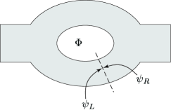
Figure 4: Ahronov-Bohm effect: the topological phase arising from the magnetic flux $\Phi$ is incorporated into the boundary conditions that relate the wave functions on two sides of an imaginary cut. The cut can be made in any place.

Aharonov-Bohm effect plays a crucial role in experimental observation and identification of $G_{Q}$ corrections (see e.g. (aron ). Therefore it must be incorporated into our scheme, and in this Section we explicate how to do this. This extends the results of Ref. stoof where AB effect was considered in superconducting circuit theory. In the following, we do not consider any orbital effects of the magnetic field but just the topological one.

Let us suppose that the nanostructure presents a closed ring threaded by a magnetic flux $\Phi$. As explained above, in presence of magnetic field the momentum operator has to be modified according to

$$i\nabla\rightarrow i\nabla-{e/\hbar}\check{\Sigma}_{H}\bm{A},$$

where $\bm{A}$ is the vector potential. Neglecting orbital effects, one can get rid of the vector potential in the Schrödinger equation by a gauge transformation. Let us have a ideal cut in the nanostructure that breaks the loop (Fig. 4.) The topological effect of the flux can be incorporated into a boundary condition for the wave-function $\psi_{L,R}$ on two sides of the cut, $\psi_{L}=\exp(i\phi_{AB}\Sigma_{H})\psi_{R}$. The phase of the wave function therefore presents a discontinuity at the cut that is equal to $\pm\phi_{AB},\phi_{AB}=\pi\Phi/\Phi_{0}$. Since the transformation does not explicitly depend on $\bm{x}$, it can be immediately extended to semiclassical Green’s functions. So that, those functions at two sides are related by

$$\check{G}_{L}=\exp(i\phi_{AB}\check{\Sigma}_{H})\check{G}_{R}\exp(-i\phi_{AB}\check{\Sigma}_{H}).$$ (40)

This solves the problem at microscopic level. Once the nanostructure has been discretized to finite elements, we note that the cut always occur between a connector and a node. The most convenient way to deal with the gauge transformation (40) is to put it into the action of the corresponding connector. To do this, we observe that the Green’s function at the right end of the connector is not $\check{G}_{R}$ of the node anymore: since the cut is crossed, it is eventually $\check{G}_{L}$ given by (40). The connector action in the presence of flux is therefore

$$S_{c}=\frac{1}{2}\sum_{n}\mbox{Tr}\ln\left[1+\frac{T_{n}}{4}(\check{G}_{c1}\check{G}_{c2}(\phi_{AB})+\right.$$

$$\left.+\check{G}_{c2}(\phi_{AB})\check{G}_{c1}-2)\right]$$ (41)

where

$$\check{G}(\phi_{AB})=\exp(i\phi_{AB}\check{\Sigma}_{H})\check{G}\exp(-i\phi_{AB}\check{\Sigma}_{H}).$$ (42)

One checks that the variation of the so-modified action reproduces the Kirchhoff laws for matrix current given in stoof . Owing to global gauge invariance, it does not matter to which connector and to which end of the connector the Aharonov-Bohm phase is ascribed. If the are more loops in the nanostructure, more connector actions have to be modified in such a way.

VII Examples

In the previous sections, we operated with general matrix ”check” structure to keep the discussion as general as possible. In this Section, we will give a set of examples to illustrate concrete applications of the technique developed. For the sake of simplicity, we choose the simplest matrix structure that gives a sensible circuit theory. We consider $2\times 2$ matrix Green’s functions whose values in two terminals can be parametrized by a single parameter $\phi$,

$$\check{G}(\phi)=\left(\begin{array}[]{cc}0&e^{-i\phi}\\ e^{i\phi}&0\end{array}\right).$$ (43)

The use of these matrix structures is that they give access to a fundamental quantity in quantum transport: Transmission distribution of transmission eigenvalues of two-terminal nanostructure. We have to explain this relation before going to concrete examples. The averaged transmission distribution is defined as

$$\rho(T)=\sum_{n}\langle\delta(T-T_{n})\rangle$$ (44)

where the sum is done over all the transport channels and the average is, in principle, to be intended over an ensemble of nanostructures of the same design. For $G\gg G_{Q}$ the transmission eigenvalues are dense in the interval $[0,1]$ and self-averaging takes place.

Let us take a connector and set Green’s functions at its ends to $\check{G}(\phi_{1}),\check{G}(\phi_{2})$. By virtue of (10) the connector action reads

$${\cal S}(\phi_{1}-\phi_{2})=\sum_{n}\ln\left[1-T_{n}\sin^{2}\frac{\phi_{1}-\phi_{2}}{2}\right].$$ (45)

The trick is to regard the whole nanostructure as a single complex connector between left and right reservoir, and set the Green’s functions in the reservoirs to $\check{G}(0),\check{G}(\phi)$. The total action (9) becomes now the connector action of the whole nanostructure and defines the transmission distribution in question,

$${\cal S}(\phi)=\int dT\rho(T)\ln\left[1-T\sin^{2}\frac{\phi}{2}\right].$$ (46)

If one computes the $\phi$-dependence of ${\cal S}$, the transmission distribution can be extracted from its analytic continuation on complex $\phi$ (NazarovOhm )

$$\rho(T)=-\frac{1}{\pi T\sqrt{1-T}}{\rm Re}\left[\frac{\partial{\cal S}}{\partial\phi}(\pi+2i\cosh^{-1}\frac{1}{\sqrt{T}}-0^{+})\right].$$ (47)

Circuit theory of the Section II gives the answer in the limit $G\gg G_{Q}$. The weak localization contribution ${\cal S}_{wl}$ gives $G_{Q}$ correction to the transmission distribution. The fluctuation contribution ${\cal S}_{G_{Q}}={\cal S}_{diff}+{\cal S}_{cooper}$ that depends on two parameters $\phi_{w,b}$, gives correlations of transmission distributions (c.f. Yuli-corrections )

$${\cal S}_{G_{Q}}(\phi_{b},\phi_{w})=\int dTdT^{\prime}\ll\rho(T)\rho(T^{\prime})\gg$$

$$\ln\left[1-T\sin^{2}\frac{\phi_{b}}{2}\right]\ln\left[1-T^{\prime}\sin^{2}\frac{\phi_{w}}{2}\right].$$ (48)

A simple application of the above formulas are $G_{Q}$ corrections to the conductance. Those are given by the derivatives of corresponding actions at $\phi_{b,w}=0$,

$$\frac{\delta G_{wl}}{G_{Q}}=-2\left.\frac{\partial^{2}{\cal S}_{wl}(\phi)}{\partial\phi^{2}}\right|_{\phi=0}$$ (49)

$$\frac{\ll G_{b}G_{w}\gg}{G^{2}_{Q}}=4\left.\frac{\partial^{4}{\cal S}_{G_{Q}}(\phi_{b},\phi_{w})}{\partial\phi_{b}^{2}\partial\phi_{w}^{2}}\right|_{\phi^{b},\phi^{w}=0}$$ (50)

VII.1 Junction Chain

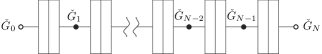
Figure 5: The chain of tunnels junctions of the same conductance $G_{T}$. In our finite-element approach, there are two Cooperon and two Diffuson eigenvalues per node. In the limit of $N\rightarrow\infty$ the chain is shown to be identical to a continous quasi-one-dimensional diffusive wire.

The first example is a chain of tunnel junctions. We will study $G_{Q}$ corrections for a chain of $N$ identical junctions that connects two reservoirs (Fig. 5.) The connector action for a tunnel junction assumes a very simple form: ${\cal S}_{c}=(G_{T}/4G_{Q}){\rm Tr}\left(\check{G}_{1c}\check{G}_{2c}\right)$, $G_{T}$ being conductance of the tunnel junction. Several tunnel junctions in series, however, provide a good approximate for diffusive wire. Therefore, in the limit $N\to\infty$ we can compare $G_{Q}$ corrections with the known results Carlo-corrections ; Yuli-corrections for corrections to transmission distribution of a one-dimensional diffusive conductor.

We set Green’s functions in the reservoirs on the left and on the right to $\check{G}(0),\check{G}(\phi)$ (c.f. Eq.43) respectively. The semiclassical action for the system reads

$${\cal S}=\frac{G_{T}}{4G_{Q}}\sum_{k=0}^{N-1}{\rm Tr}\check{G}_{k}\check{G}_{k+1}-\frac{i\pi}{\delta_{S}}\sum_{k=1}^{N-1}{\rm Tr\check{\Sigma}_{k}\check{G}_{k}},$$ (51)

Here $k=1,\dots,N-1$ labels the nodes, while $k=0$ and $k=N$ identify left and right reservoir respectively. All the nodes are assumed to be identical with the same $\delta_{S}$.

Since all the junctions are identical, the semiclassical solution is easy to find: the ”phase” $\phi$ drops by the same amount at each junction, and the solution reads $\check{G}_{k}=\check{G}(k\phi/N)$, provided $\check{\Sigma}_{k}\propto\check{1}$ within each $2\times 2$ block. This gives the optimal value of the action,

$${\cal S}=\frac{NG_{T}}{2G_{Q}}\cos\left(\frac{\phi}{N}\right)$$ (52)

from which one can evaluate the semiclassical transmission distribution by using relation (47). In the limit $N\to\infty$ ${\cal S}=-({G_{D}}/{4G_{Q}})\phi^{2}$, $G_{D}\equiv G_{T}/N$ being the conductance of the whole chain. This gives well-known transmission distribution for diffusive conductor, $\rho(T)=(G_{D}/2G_{Q})/T\sqrt{1-T}$ NazarovOhm .

As explained above, to calculate $G_{Q}$ corrections we augment the ”check” dimension of the Green’s functions by introducing the ”black” and ”white” structure. Consequently, the parameter $\phi$ gets a ”color” index $b$ or $w$. The semiclassical solution for resulting $4\times 4$ matrix is non-zero in $bb$ and $ww$ blocks,

$$\check{G}^{0}_{k}=\left(\begin{array}[]{cc}\check{G}(k\phi_{b}/N)&0\\ 0&\check{G}(k\phi_{w}/N)\end{array}\right).$$ (53)

Now we shall derive the matrix $\hat{M}$ eigenvalues of which determine $G_{Q}$ corrections. It is advantageous to use a parametrization of the deviations from the semiclassical solution,$\check{g}$, which automatically satisfy $\check{g}\check{G}+\check{G}\check{g}=0$ in each node. To this end, we rewrite the action (51) in a special basis: That one where $\check{G}^{0}_{k}$ are diagonal in each node,

$$\check{G}^{0}_{k}=\left(\begin{array}[]{cccc}1&0&0&0\\ 0&-1&0&0\\ 0&0&1&0\\ 0&0&0&-1\end{array}\right).$$ (54)

Then the deviation of the form

$$\check{g}_{k}=\left(\begin{array}[]{cccc}0&0&0&g^{bw}_{k,p}\\ 0&0&g^{bw}_{k,m}&0\\ 0&g^{wb}_{k,p}&0&0\\ g^{wb}_{k,m}&0&0&0\end{array}\right)$$ (55)

satisfies the condition mentioned.

In this basis (see Appendix A for details) the action reads

$${\cal S}=\frac{G_{T}}{2G_{Q}}\sum_{k=0}^{N-1}{\mbox{T}r}\check{G}_{k}\check{L}\check{G}_{k+1}\check{L}^{-1}-\frac{i\pi}{\delta_{S}}\sum_{k=1}^{N-1}{\mbox{T}r}\check{\Sigma}_{k}\check{G}_{k},$$ (56)

where $bb$ $(ww)$ block of $\check{L}$ is given by

$$L^{bb(ww)}=\left(\begin{array}[]{cc}\cos(\phi^{b(w)}/N)&i\sin(\phi^{b(w)}/N)\\ i\sin(\phi^{b(w)}/N)&\cos(\phi^{b(w)}/N)\end{array}\right).$$ (57)

We expand the Green’s matrices according to Eq. (30), write the quadratic form in terms of $\check{g}$ and diagonalize it (see Appendix A) to find the following set of eigenvalues, ($l=1\dots N-1$)

$$\frac{4G_{Q}}{G_{T}}M^{\pm}_{l}(\phi^{b},\phi^{w})=2\cos\frac{\phi^{b}}{2N}\cos\frac{\phi^{w}}{2N}\cos\frac{\pi l}{N}-\cos\frac{\phi^{b}}{N}$$

$$-\cos\frac{\phi^{w}}{N}\mp\sqrt{4\sin^{2}\frac{\phi^{b}}{2N}\sin^{2}\frac{\phi^{w}}{2N}\cos^{2}\frac{\pi l}{N}+\epsilon^{2}},$$ (58)

$\epsilon\equiv 2\pi G_{Q}(\Sigma^{b}-\Sigma^{w})/G_{T}i\delta_{S}$ measures the difference of Green’s function energy parameter in $bb$ and $ww$ blocks in units of a single-node Thouless energy. To obtain eigenvalues that determine the weak localization contribution, we set $\phi^{w}=-\phi^{b}=\phi,\epsilon=0$. This yields

$$M^{+}_{wl,l}(\phi)=\frac{G_{T}}{4G_{Q}}\cos(\frac{\phi}{N})\left[\cos\frac{\pi l}{N}-1\right]$$ (59)

$$M^{-}_{wl,l}(\phi)=\frac{G_{T}}{4G_{Q}}\left[\cos\frac{\pi l}{N}-\cos\frac{\phi}{N}\right]$$ (60)

Let us discuss the weak localization correction first. If we neglect decoherence factors, we can sum up over $l$ to find a compact analytical expression

$${\cal S}_{wl}=\frac{(N-2)}{2}\ln(\cos\frac{\phi}{N})+\frac{1}{2}\ln\left(\frac{\sin\frac{2\phi}{N}}{\sin\phi}\right)$$ (61)

In the limit $N\to\infty$ this reproduces the known correction for one-dimensional diffusive wire Yuli-corrections ,

$${\cal S}_{wl}=\frac{1}{2}\ln\left(\frac{\phi}{\sin\phi}\right)$$ (62)

It is interesting to note that the weak localization correction is absent for $N=2$. We will see below that this is a general property of a single-node tunnel-junction system. It was observed in Yuli-corrections that a part of weak localization correction in diffusive conductors is universal: It depends neither on the shape nor on the dimensionality of the conductor. The universal part is concentrated near transmissions close to one and is given by

$$\delta\rho_{wl}(T)=-\frac{1}{4}\delta(T-1),$$ (63)

while the non-universal part is a smooth function of $T$. The relation (61) possesses this property at any $N$, since the universal part comes from the divergency in (61) at $\phi=\pi$ where the eigenvalue $M^{-}_{wl,1}$ goes to zero. Our approach proves that this correction is universal for a large class of the nanostructures, not limited to diffusive ones, for any nanostructure where transmission eigenvalues approach $1$. This is guaranteed by the logarithmic form of the action. If $M^{-}_{wl,1}\propto(\pi-\phi)$ at $\phi\to\pi$, the correction is given by (63) irrespective of the proportionality coefficient.

Expanding (61) at $\phi\to 0$ we find the correction to the conductance of the tunnel junction chain,

$$\frac{\delta{G}_{wl}}{G_{Q}}=-\frac{1}{3}\frac{(N-1)(N-2)}{N^{2}}$$ (64)

This is written for orthogonal ensemble, a well-known factor $(1-2/\beta)$ defines the correction for other pure ensembles. The effect of spin and magnetic decoherence can be taken into account by shifting the eigenvalues (59 ,60) according to Eq. 39 since the decoherence factors in each node are the same, $\zeta_{H,so}\equiv\eta_{H,so}(4G_{Q}/G_{T})$.

The ${\cal S}_{wl}$ is still given by analytical although lengthy expression (See Appendix A). The correction to the transmission distribution corresponding to this expression is plotted in Fig. 6 for different strengths of spin-orbit coupling to illustrate the transition between the orthogonal and simplectic ensembles. The correction to the conductance is given by

$$\frac{\delta G_{wl}}{G_{Q}}=3F(N,\zeta_{H}+\zeta_{so})-F(N,\zeta_{H})$$ (65)

where we define an auxiliary function $F(x,N)$

$$F(x,N)=-\frac{(N-1)}{N^{2}}-\frac{1}{N^{2}}\frac{(2+x)^{2}}{x(4+x)}\\ -\frac{1}{N\sqrt{x(4+x)}}\frac{2^{2N}+\left(2+x+\sqrt{x(4+x)}\right)^{2N}}{2^{2N}-\left(2+x+\sqrt{x(4+x)}\right)^{2N}}$$

Let us discuss the parametric correlations. Without decoherence factors and at the same energy ($\epsilon=0$) one can still sum up over the modes to obtain an analytical expression,

$${\cal S}_{Diff}={\cal S}_{Coop}=(N-1)\ln\left(\cos\frac{\phi_{b}}{N}+\cos\frac{\phi_{w}}{N}\right)+\\ +\sum_{\pm}\ln\left(\frac{\sin\frac{\phi_{b}\pm\phi_{w}}{2}}{\sin\frac{\phi_{b}\pm\phi_{w}}{2N}}\right)$$ (66)

The fluctuation of conductance obtained with (50) reads

$$\frac{\langle\langle\delta G^{2}\rangle\rangle}{G^{2}_{Q}}=\frac{2}{15}\frac{N^{4}+15N-16}{N^{4}}$$ (67)

and converges to the known expression for quasi-one-dimensional diffusive conductor at $N\to\infty$. We notice that this convergence is rather quick, the fluctuation at $N=5$ differs from asymptotic value by $10\%$ only. We see thus that the diffusive wire, that in principle contains an infinite number of Cooperon and Diffuson modes, can be, with sufficient accuracy, described by the finite-element technique even at low number of elements.

Another point to discuss concerns the correlations of transmission eigenvalues $T_{n}$, those can be obtained by analytic calculation of (VII). It is instructive to concentrate on the relatively small eigenvalue separations those are much smaller than $1$ but still exceed an average spacing $\simeq G_{Q}/G$ between the eigenvalues, $G_{Q}/G\ll|T-T^{\prime}|\ll 1$. We observe that the correlation in this case is determined by the divergency of ${\cal S}$ at $\phi_{b}-\phi_{w}\to\pm 2\pi$. Indeed, $M^{-}_{1}$ approaches $0$ in this limit. This again suggest the universality of these correlations. Indeed, as shown in Yuli-corrections for diffusive conductors, the correlations in this parameter range are determined by universal Wigner-Dyson statistics and reduce to

$$\langle\langle\rho(T)\rho(T^{\prime})\rangle\rangle=-\frac{2}{\pi^{2}\beta}{\rm Re}\frac{1}{(T-T^{\prime}+i0^{+})^{2}}.$$ (68)

Since the conductance fluctuations are contributed by correlations of $T_{n}$ at scale $\sim 1$ as well, they are not universal. We plot in Fig. 7 the correlator of conductance fluctuations as function of energy difference at several $N$.

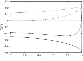
Figure 6: Weak localization correction to the transmission distribution of a system of four identical junctions at different values of spin-orbit parameter $\zeta_{SO}$. We plot here cumulate correction $X(T)\equiv\int_{T}^{1}dT^{\prime}T^{\prime}\delta\rho(T^{\prime})$. $X(1)$ represents the universal singular part of the correction (c.f. Eq. 63) while $X(0)$ gives correction to the conductance. The lowest curve corresponds to strictly zero $\zeta_{SO}$ and therefore represents pure orthogonal ensemble. Its negative value at $T=1$ is partially compensated by positive non-universal contribution coming from $T\simeq 1$ so that the resulting correction to conductance $\delta G_{wl}/G_{Q}=X(0)\approx 0.2$. The two higher curves correspond to relatively small values of $\zeta_{SO}$, $0.05$ and $0.4$. While they are close to the orthogonal ensemble result at $T\simeq 1$, their behavior at $T\approx 1$ is quite different: the universal correction is that of symplectic ensemble and is of positive sign. The highest curve corresponding to $\zeta_{SO}=10$ is close the cumulate correction of pure symplectic ensemble, $X_{sym}(T)=-X_{ort}(T)/2$.

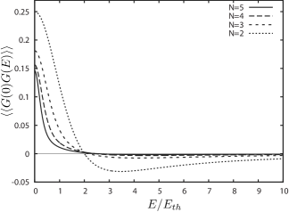
Figure 7: Energy dependence of the correlator of conductance fluctuations $\ll G(0)G(E)\gg$ for chains with different number of junctions $N$. The energy difference is normalized to Thouless energy of the whole chain, $E_{th}\equiv\delta_{s}G_{T}/2\pi G_{Q}N^{2}$. Note the fast convergence of the correlator to that of diffusive wire for big $N$ and negative correlations at large $E$.

VII.2 AB ring

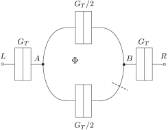
Figure 8: A simplest circuit to exemplify AB effect consists of two nodes and for (tunnel) connectors. AB phase modifies the Green’s function on the right side of the lowest connector with respect to $\check{G}_{B}$. The cut is given by dotted line.

In this subsection we exemplify evaluation of $AB$ effect within our scheme. We concentrate on the simple circuit presented in Fig. 8. It contains four tunnel junctions and two nodes labeled $A$ and $B$. The conductances of the junctions are chosen to re-use the results of the previous section for a chain of three tunnel junctions: The solution of semiclassical circuit theory equations is given by (53) for $N=3$. The action reads

$$S=\frac{G_{T}}{4G_{Q}}{\mbox{T}r}\left\{\check{G}_{L}\check{G}_{A}+\frac{1}{2}\check{G}_{A}\check{G}_{B}\right.$$

$$\left.+\frac{1}{2}\check{G}_{A}\check{G}_{B}(\phi_{AB})+\check{G}_{B}\check{G}_{R}\right\}-i\frac{\pi}{\delta}\sum_{i=A,B}{\mbox{T}r}\check{\Sigma}_{i}\check{G}_{i}.$$ (69)

where $\check{G}_{L,R}$ are Green’s functions in the reservoirs and $\check{G}_{B}(\phi_{AB})$ is modified according to Eq. 40. To study correlation of conductance fluctuations, we consider different Green’s functions for white and black block, and subjected to different fluxes $\phi_{AB}^{b}\neq\phi_{AB}^{w}$. For weak localization correction, we set $\phi_{AB}^{b}=-\phi_{AB}^{w}=\phi_{AB}$

To calculate the matrix $\hat{M}$ we use again the basis where $G^{(0)}_{i}$ are diagonal and the parametrization for $\check{g}$ introduced in the previous subsection. It reads

$$M=\left(\begin{array}[]{cc}M_{d}&M_{od}\\ M^{*}_{od}&M_{d}\end{array}\right)$$

where $2\times 2$ blocks $M_{d,od}$ are given

$$\frac{G_{T}M_{d}}{4G_{Q}}=\left(\begin{array}[]{cc}-\cos\varphi^{b}-\cos\varphi^{w}+\epsilon&0\\ 0&-\cos\varphi^{b}-\cos\varphi^{w}-\epsilon\end{array}\right)$$

$$\frac{G_{T}M_{od}}{4G_{Q}}=\frac{1+e^{i(\phi_{AB}^{b}-\phi_{AB}^{w})}}{2}\left(\begin{array}[]{cc}\cos\frac{\varphi^{b}}{2}\cos\frac{\varphi^{w}}{2}&\sin\frac{\varphi^{b}}{2}\sin\frac{\varphi^{w}}{2}\\ \sin\frac{\varphi^{b}}{2}\sin\frac{\varphi^{w}}{2}&\cos\frac{\varphi^{b}}{2}\cos\frac{\varphi^{w}}{2}\end{array}\right)$$

The parameter $\epsilon$ which characterizes the energy difference between black and white Green’s function is defined as in the previous subsection. At $\epsilon=0$ we obtain explicit expression for the Diffuson eigenvalues (the Cooperon ones are obtained by $\phi^{w}\rightarrow-\phi^{w}$ and $\phi_{AB}^{w}\rightarrow-\phi_{AB}^{w}$),

$$\frac{4G_{Q}}{G_{T}}M_{1,2}^{+}=-\cos\frac{\phi_{b}}{3}-\cos\frac{\phi_{w}}{3}$$

$$\pm\cos\left(\frac{\phi^{b}_{AB}-\phi^{w}_{AB}}{2}\right)\cos\left(\frac{\phi_{b}-\phi_{w}}{6}\right),$$ (72)

$$\frac{4G_{Q}}{G_{T}}M_{1,2}^{-}=-\cos\frac{\phi_{b}}{3}-\cos\frac{\phi_{w}}{3}$$

$$\pm\cos\left(\frac{\phi^{b}_{AB}-\phi^{w}_{AB}}{2}\right)\cos\left(\frac{\phi_{b}+\phi_{w}}{6}\right).$$ (73)

The weak localization correction to the action reads

$${\cal S}_{wl}(\phi)=\frac{1}{2}\ln\left(\frac{\cos^{2}(\phi/3)(4-\cos^{2}(\phi_{AB}))}{4\cos^{2}(\phi/3)-\cos^{2}(\phi_{AB})}\right),$$ (74)

from which we calculate the correction to conductance as function of the flux

$$\frac{\delta G_{wl}}{G_{Q}}=-\frac{4\cos^{2}(\phi_{AB})}{9(7-\cos(2\phi_{AB}))}.$$ (75)

We see that the weak localization correction cancels at half-integer flux $\phi_{AB}=\pi$. This is because the junctions forming the loop are taken to be identical. The flux dependence exhibits higher harmonics indicating semiclassical orbits that encircle the flux more than once.

For the correlator of conductance fluctuations we obtain

$$\frac{\langle\delta G^{2}\rangle}{G^{2}_{Q}}=\sum_{\pm}\frac{259-4\cos(\phi^{w}_{AB}\pm\phi^{b}_{AB})+\cos 2(\phi^{w}_{AB}\pm\phi^{b}_{AB})}{81(\cos(\phi^{w}_{AB}\pm\phi^{b}_{AB})-7)^{2}}$$ (76)

where plus and minus signs indicate Cooperon and Diffuson contributions respectively. The higher harmonics are present as well.

VII.3 Two connectors and one node

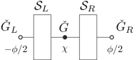
Figure 9: The simplest possible circuit comprises one node, two connectors($L$ and $R$), and two reservoirs where Green’s functions $\check{G}_{L,R}$ are fixed.

Probably the simplest system to be considered by circuit theory methods consists of a single node and two connectors (Fig. 9). Since in this case there are only $N_{ch}$ eigenvalues, one can straightforwardly elaborate on complicated arbitrary connectors. For this setup we are still able to find an analytical expression for Cooperon and Diffusion eigenvalues. This allows us to get an expression for the weak localization correction to the conductance which was vanishing in the case of two tunnel junctions. Each connector is in principle characterized by the distribution of transmission coefficients $\{T^{R}_{n}\}$, $\{T^{L}_{n}\}$, or, equivalently, by the functional form of the connector action given by Eq. (10), ${\cal S}_{L},{\cal S}_{R}$ . The action for the whole system reads

$${\cal S}={\cal S}_{L}(\check{G}_{L},\check{G})+{\cal S}_{R}(\check{G},\check{G}_{R})-i\frac{\pi}{\delta_{s}}{\rm Tr}\check{\Sigma}\check{G}.$$ (77)

$\check{G}$ being the Green’s function of the node. We employ $2\times 2$ matrices parametrized by (43), and set the Green’s functions in the left and right reservoir to $\check{G}(-\phi/2)$ and $\check{G}(\phi/2)$ respectively. The saddle-point value of $\check{G}$ is given by the phase $\chi$ and for a general choice of ${\cal S}_{L}$ and ${\cal S}_{R}$ does depend on $\phi$, $\chi\equiv\chi(\phi)$. The total action in the saddle point is therefore ${\cal S}(\phi)={\cal S}_{L}(\chi+\phi/2)+{\cal S}_{R}(\chi-\phi/2)$. We expand the Green’s function according to Eq. 30. The second order correction to the action in this case reads

$${\cal S}^{(2)}=-i\frac{\pi}{\delta_{s}}\mbox{Tr}\,\check{\Sigma}\,\check{g}\\ -\frac{1}{2}\sum_{n}\mbox{Tr}\Bigg{\{}\frac{T^{L}_{n}}{4[1+\frac{T^{L}_{n}}{4}(\{\check{G}^{0},\check{G}_{L}\}-2)]}\check{g}^{2}\check{G}^{0}\check{G}_{L}\\ +\left[\frac{T^{L}_{n}}{4[1+\frac{T^{L}_{n}}{4}(\{\check{G}^{0},\check{G}_{L}\}-2)]}\right]^{2}\ (\check{g}\check{G}_{L}\check{g}\,\check{G}_{L}+\check{g}^{2})+(L\leftrightarrow R)\Bigg{\}}.$$ (78)

Acting like in the previous subsections, we find two following Diffuson eigenvalues (the Cooperon ones are obtained by the substitution $\phi^{w}\rightarrow-\phi^{w}$).

$$M^{\pm}(\phi^{b},\phi^{w})=\sum_{i=b,w}I(\phi^{i})\left[\cot[\chi(\phi^{i})-\frac{\phi^{i}}{2}]-\cot[\chi(\phi^{i})+\frac{\phi^{i}}{2}]\right]\\ -\frac{1-\cos[\chi(\phi^{b})+\frac{\phi^{b}}{2}\mp\chi(\phi^{w})\mp\frac{\phi^{w}}{2}]}{2}\sum_{i=b,w}\left\{\frac{1}{\sin^{2}[\chi(\phi^{i})+\phi^{i}/2]}\left[\frac{I^{\prime}(\phi^{i})}{\chi^{\prime}(\phi^{i})+1/2}-I(\phi^{i})\cot[\chi(\phi^{i})+\frac{\phi^{i}}{2}]\right]\right\}\\ +\frac{1-\cos[\chi(\phi^{b})-\frac{\phi^{b}}{2}\mp\chi(\phi^{w})\pm\frac{\phi^{w}}{2}]}{2}\sum_{i=b,w}\left\{\frac{1}{\sin^{2}[\chi(\phi^{i})-\phi^{i}/2]}\left[\frac{I^{\prime}(\phi^{i})}{\chi^{\prime}(\phi^{i})-1/2}-I(\phi^{i})\cot[\chi(\phi^{i})-\frac{\phi^{i}}{2}]\right]\right\}.$$ (79)

Here we introduce $I(\phi)\equiv\partial{\cal S}/{\partial\phi}$ to characterize the derivative of the total semiclassical action. We see that $M^{-}$ approaches zero in the limit $\phi_{b},\phi_{w}\to\pm\pi,\mp\pi$ provided $I(\phi)$ stays finite. As discussed, this divergency guarantees the universality of the correlations of transmission eigenvalues.

Below we specify to three different cases.

VII.3.1 Symmetric setup

If we set ${\cal S}_{R}={\cal S}_{L}$, $\chi(\phi^{b(w)})$ is zero regardless the concrete form ${\cal S}_{L}$. The total action therefore reads ${\cal S}(\phi)=2{\cal S}_{L}(\phi/2)$. The eigenvalues (79) take a simpler form. To compute the weak localization correction to the action we set $\phi^{b}=-\phi^{w}=\phi$ to find

$${\mathcal{S}}_{wl}=\frac{1}{2}\ln\left(\frac{I^{\prime}(\phi)}{I(\phi)}\tan\frac{\phi}{2}\right)+{\rm const}.$$ (80)

For tunnel junctions, $I(\phi)\propto\sin(\phi/2)$ and the correction disappears.

Expanding Eq. 80 in Taylor series near $\phi\rightarrow 0$ we reproduce the well-known result of Iida for weak localization correction to conductance. To comply with the notations used there, we characterize connectors with $t_{p}=\sum_{n}T_{n}^{p}$.

$$\frac{\delta G_{wl}}{G_{Q}}=-\frac{t_{2}}{4t_{1}},$$ (81)

Similar expansion of Diffusion and Cooperon eigenvalues reproduces the result of Iida for conductance fluctuations,

$$\frac{\langle(\delta G)^{2}\rangle}{G_{Q}}=\frac{3t_{2}^{2}+2t_{1}^{2}-2t_{1}(t_{2}+t_{3})}{8t_{1}^{2}}.$$ (82)

VII.3.2 Diffusive connectors

It is instructive for understanding circuit theory of $G_{Q}$ corrections to specify the relation (80) to diffusive connectors. Since in this case $I(\phi)\propto\phi$, we obtain

$${\cal S}_{wl,node}=\frac{1}{2}\ln(\tan(\phi/2)/\phi)$$ (83)

Two connectors, single node situation can be easily realized in a quasi-one-dimensional wire with inhomogeneous resistivity distribution along the wire. A low-resistivity region would make a node if bounded by two shorter resistive regions that would make the connectors. On the other hand it has been proven in Yuli-Annalen that the weak localization correction in inhomogeneous wires does not depend on the resistivity distribution. Therefore, it has to be universally given by (62), ${\cal S}_{wl,1d}=(1/2)\ln(\phi/\sin\phi)\neq{\cal S}_{wl,node}$. How to understand this apparent discrepancy?

This illustrates a very general point: $G_{Q}$ corrections may be accumulated at various space scales ranging from mean free path to sample size. The experimental observation of the corrections relies on the ability to separate the contributions coming from different scales, e.g. by changing magnetic field bergman . With our approach, we evaluate the part coming from interference at the scale of the node. The part coming from interference at shorter scale associated with the connectors is assumed to be included into transmission distribution of these connectors.

For our particular setup, this extra contribution comes from two identical connectors. Since only half of the phase $\phi$ drops at each connector, the contribution equals $2{\cal S}_{wl,1d}(\phi/2)$. Summing up both contributions, we obtain

$${\cal S}_{wl,node}+2{\cal S}_{wl,1d}(\phi/2)={\cal S}_{wl,tot}={\cal S}_{wl,1d}(\phi)$$

That is, the weak localization correction in this case remains universal provided the contribution of the node is augmented by contributions of two connectors.

VII.3.3 Non-ideal Quantum Point Contact

The transmission distribution of an ideal multi-mode Quantum Point Contact (QPC) with conductance $G_{B}\gg G_{Q}$ is very degenerate since all $T_{n}=1$ or $0$. This degeneracy is lifted if the QPC is adjacent to a disordered region, even if the scattering in this region is weak. This can be modeled as a connector with conductance $G_{D}\gg G_{B}$ in series.

The weak localization correction to the conductance has been calculated already a while ago (Beenakker-QPC ). In the relevant limit, it is parametrically small in comparison with $G_{Q}$, $\delta G_{wl}=-G_{Q}(G_{B}/G_{D})$. Usual way to verify the applicability of semiclassical approach to quantum transport is to compare the conductance of a nanostructure with the weak localization correction to it. For generic nanostructure, this gives $G\gg G_{Q}$. However, for our particular example $\delta G_{wl}\ll G_{B}$ even for a few-channel QPC where $G_{B}\simeq G_{Q}$. So the question is: Is semiclassical approach really valid at $G_{B}\simeq G_{Q}$?

To answer this question, we compute the weak localization correction to the transmission distribution. Since system is not symmetric, we make use of the full expression (79). In the limit of $G_{D}\gg G_{B}$, the relevant values of $\phi$ are close to $\pi$. We stress it by shifting the phase, $\mu=\pi-\phi,|\mu|\ll 1$.

The circuit theory analysis in semiclassical limit gives campagnano

$$I(\mu)=G_{D}(-\frac{\mu}{2}+\sqrt{\frac{\mu^{2}}{4}+R_{c}})\hskip 28.45274pt\chi=\frac{\pi}{2}+\sqrt{\frac{\mu^{2}}{4}+R_{c}},$$

where $R_{c}\equiv 4G_{B}/G_{D}\ll 1$. This gives to the following distribution of reflection coefficients (c.f. Eq. 47)

$$\rho(R)=\frac{G_{D}}{2\pi G_{Q}}\Theta(R_{c}-R)\sqrt{\frac{R_{c}}{R}-1}.$$

We use the above relations with (79) to find the Cooperon eigenvalues,

$$M^{+}(\mu) = -G_{D}\left(-\frac{1}{2}+\frac{\mu/4}{\sqrt{\frac{\mu^{2}}{4}+R_{c}}}\right)\frac{\frac{\mu^{2}}{4}+R_{c}}{R_{c}/2},$$ (84)

$$M^{-}(\mu) = G_{D}\left(-\frac{\mu}{2}+\sqrt{\frac{\mu^{2}}{4}+R_{c}}\right)\frac{\mu}{2R_{c}}.$$ (85)

This yields the weak localization correction to the current,

$$I_{wl}(\mu)=\frac{2R_{c}}{\mu(\mu^{2}+4R_{c})}.$$

The resulting correction to the transmission distribution consists of two delta-functional peaks of opposite sign, those are located at the edges of the semiclassical distribution,

$$\delta\rho_{wl}(R)=\frac{1}{4}\left[\delta(R-R_{c})-\delta(R)\right].$$ (86)

To estimate the conditions of applicability, we smooth the correction at the scale of $R_{c}$. This gives $|\delta\rho|/\rho\simeq G_{Q}/G_{B}$ and the semiclassical approach does not work at $G_{B}\simeq G_{Q}$. This agrees with RMT arguments given in campagnano . The correction to the conductance calculated with (86) agrees with the value cited above and indeed is anomalously small.

VIII Conclusions

We present a finite-element method to evaluate quantum corrections — typically of the order of $G_{Q}$ — to transport characteristics of arbitrary nanostructures. This includes universal conductance fluctuation and weak localization. We work with matrix Green’s functions of arbitrary structure to treat a wider class of problems that includes superconductivity, full counting statistics and non-equlibrium transport. At microscopic level, the corrections are expressed in terms of Diffuson and Cooperon modes of continuous Green’s functions. We employ a variational method based on an action to formulate a consistent finite-element approach.

We illustrate the method with a set of simple and physically interesting examples. All examples are based on $2\times 2$ matrices, this suffices to calculate the transmission distribution of two-terminal structures. We show how a chain of tunnel junctions approaches the diffusive wire upon increasing the number of junctions and study transitions between ideal RMT ensembles in the chain. We consider the simplest finite-element system that exhibits Ahronov-Bohm effect. We obtain general results for a single-node system with two arbitrary connectors and check their consistence with the well-known results for quantum cavity. This allows us to improve understanding of quantum interference in inhomogeneous diffusive wires and non-ideal quantum point-contacts.

Appendix A Junction chain

In this Appendix we illustrate how to find the eigenvalues of the matrix $M$ defined in section IV for the chain of tunnel junctions introduced. We consider the action in the rotated basis presented in text

$${\cal S}=\frac{G_{T}}{4G_{Q}}\sum_{i=0}^{N}{\mbox{T}r}\check{G}_{i}\check{L}\check{G}_{i+1}\check{L}^{-1}-\frac{i\pi}{\delta_{s}}\sum_{i=1}^{N-1}{\mbox{T}r}\check{\Sigma}_{i}\check{G}_{i}.$$ (87)

We expand the Green’s matrices according to Eq. (30)

The second order correction to the action reads (the first order is zero because we perform the expansion around the stationary point)

$${\cal S}^{(2)}=\frac{G_{T}}{4G_{Q}}\sum_{i=0}^{N}{\rm Tr}\left\{\check{g}_{i}\check{L}\check{g}_{i+1}\check{L}^{-1}-\frac{1}{2}\check{g}_{i}\check{L}\check{G}^{0}_{i+1}\check{L}^{-1}-\frac{1}{2}\check{G}^{0}_{i}\check{L}\check{g}_{i+1}\check{L}^{-1}\right\}-\frac{i\pi}{\delta_{s}}\sum_{i=1}^{N-1}{\rm Tr}\left\{\delta\check{\Sigma}_{i}\check{g}_{i}-\frac{1}{2}\check{\Sigma}_{i}\check{g}^{2}_{i}\check{G}_{i}^{0}\right\}$$ (88)

Taking the variation respect to $g^{wb}_{p,k}$ and $g^{wb}_{m,k}$ leads to the eigenvalue equations the matrix $M$.

$$\sin\frac{\phi^{b}}{2N}\sin\frac{\phi^{w}}{2N}(g^{wb}_{p,k+1}+g^{wb}_{p,k-1})+\cos\frac{\phi^{b}}{2N}\cos\frac{\phi^{w}}{2N}(g^{wb}_{m,k+1}+g^{wb}_{m,k-1})-(\cos\frac{\phi^{b}}{N}+\cos\frac{\phi^{w}}{N})g^{wb}_{m,k}\\ -\frac{1}{2\xi}(\Sigma^{b}-\Sigma^{w})g^{wb}_{m,k}-\frac{4G_{Q}}{G_{T}}Mg^{wb}_{m,k}=0,$$ (89)

$$\sin\frac{\phi^{b}}{2N}\sin\frac{\phi^{w}}{2N}(g^{wb}_{m,k+1}+g^{wb}_{m,k-1})+\cos\frac{\phi^{b}}{2N}\cos\frac{\phi^{w}}{2N}(g^{wb}_{p,k+1}+g^{wb}_{p,k-1})-(\cos\frac{\phi^{b}}{N}+\cos\frac{\phi^{w}}{N})g^{wb}_{p,k}\\ +\frac{1}{2\xi}(\Sigma^{b}-\Sigma^{w})g^{wb}_{p,k}-\frac{4G_{Q}}{G_{T}}Mg^{wb}_{p,k}=0,$$ (90)

where $\xi=i\delta_{s}\,G_{T}/(4\pi G_{Q})$. To solve the system of coupled equations it is convenient to write

$$g^{wb}_{p,k}=g^{>}_{p}e^{iqk}+g^{<}_{p}e^{-iqk},$$ (91)

and similar equation for the $m$-component. The coefficient $q$ is to be determined from the boundary conditions

$$g^{wb}_{p,0}=0,$$

$$g^{wb}_{p,N}=0.$$

From the boundary conditions we have $g^{>}_{k}=-g^{<}_{k}$ and $q=\pi l/N$ with $l=1,..,N-1$. We substitute the expressions 91 in the equations for the eigenvalues and get

$$\frac{4G_{Q}}{G_{T}}M^{\pm}_{l}(\phi^{b},\phi^{w})=2\cos\frac{\phi^{b}}{2N}\cos\frac{\phi^{w}}{2N}\cos(\frac{\pi l}{N})-\cos\frac{\phi^{b}}{N}$$

$$-\cos\frac{\phi^{w}}{N}\mp\sqrt{4\sin^{2}\frac{\phi^{b}}{2N}\sin^{2}\frac{\phi^{w}}{2}\cos^{2}(\frac{\pi l}{N})+\epsilon^{2}}$$ (92)

The quantity $\epsilon$ being $(\Sigma^{b}-\Sigma^{w})/2\xi$.

Here we report the correction to the action when decoherence and spin orbit are present as generalization of Eq. 61 , let us define the following functions

$$s_{1}(\phi,x,N)=\frac{1}{2}\left(2+\frac{x}{\cos(\phi/N)}\right)\\ +\sqrt{\frac{1}{4}\left(2+\frac{x}{\cos(\phi/N)}\right)^{2}-1}$$

$$s_{2}(\phi,x,N)=\frac{1}{2}\left(x+2\cos(\phi/N)\right)\\ +\sqrt{\frac{1}{4}\left(x+2\cos(\phi/N)\right)^{2}-1}$$

and the function

$$A(\phi,x,N)=\\ \left[\frac{s_{1}^{2}-s_{1}^{-2}}{2-s_{1}^{2}-s_{1}^{-2}}+N\frac{-s_{1}^{2N}+s_{1}^{-2N}}{2-s_{1}^{2N}-s_{1}^{-2N}}\right]\frac{\partial}{\partial\phi}\ln\left(s_{1}(\phi,x,N)\right)\\ -\left[\frac{s_{2}^{2}-s_{2}^{-2}}{2-s_{2}^{2}-s_{2}^{-2}}+N\frac{-s_{2}^{2N}+s_{2}^{-2N}}{2-s_{2}^{2N}-s_{2}^{-2N}}\right]\frac{\partial}{\partial\phi}\ln\left(s_{2}(\phi,x,N)\right)$$

We can finally express the correction to the action as

$$\frac{\partial}{\partial\phi}{\cal S}_{wl}(\phi)=A(\phi,\zeta_{H},N)-3A(\phi,\zeta_{H}+\zeta_{so},N)$$ (93)

References

- (1) L. P. Gor’kov, A. I. Larkin and D. E. Khmel’nitskii, Pis’ma Zh. Eksp. Teor. Fiz. 30, 248 (1979) [JETP Lett. 30, 228 (1979)]; E. Abrahams, P. W. Anderson, D. C. Licciardello, and T. V. Ramakrishnan, Phys. Rev. Lett. 42, 673 (1979).
- (2) B. L. Altshuler, Pis’ma Zh. Eksp. Teor. Fiz. 41, 530 (1985) [JETP Lett. 41, 648 (1985)]; P. A. Lee and A. D. Stone, Phys. Rev. Lett. 35, 1622 (1985); B. L. Altshuler and D. E. Khmelnitskii, JETP Lett. 42, 559 (1985).
- (3) S. Washburn and R. A. Webb, Rep. Prog. Phys. 55, 1311 (1992).
- (4) G.Bergman, Phys. Rep. 107, 1 (1984).
- (5) P. A. Lee and T. V. Ramakrishnan, Rev. Mod. Phys. 57, 287 (1987).
- (6) P. A. Lee, A. D. Stone, and H. Fukuyama, Phys. Rev. B 55, 1039 (1987).
- (7) Y. Imry, Europhys. Lett. 1, 249 (1986).
- (8) C. W. J. Beenakker, Rev. Mod. Phys. 69, 731 (1997)
- (9) R. Blümel and L. Smilansky , Phys. Rev. Lett. 60, 477 (1988).
- (10) Yu. V. Nazarov, in: Quantum Dynamics of Submicron Structures, ed. by H. A. Cerdeira, B. Kramer, and G. Schön, Kluwer Academic Publishers, Dordrecht (1995), p.687.
- (11) K.B. Efetov, Adv. Phys. 32, 53 (1983).
- (12) M.R.Zirnbauer, Nucl. Phys B 265 375 (1986).
- (13) S. Iida, H. A. Weidenmueller, and J. A. Zuk, Ann. Phys. (N.Y.) 200, 219 (1990).
- (14) C. W. J. Beenakker, Phys. Rev. B 49, 2205 (1994); C. W. J. Beenakker, Phys. Rev. Lett. 70, 4126 (1993).
- (15) Yu. V. Nazarov, Phys. Rev. B 52, 4720 4723 (1995); Yu. V. Nazarov, Phys. Rev. Lett. 76, 2129 (1996).
- (16) Yu. V. Nazarov, Phys. Rev. Lett. 73, 1420 (1994).
- (17) Yu. V. Nazarov and D. A. Bagrets, Phys. Rev. Lett. 88, 196801 (2002).
- (18) Yu. V. Nazarov, Phys. Rev. Lett. 73, 134 (1994).
- (19) A. Brataas, Yu. V. Nazarov, and G. E. W. Bauer Phys. Rev. Lett. 84, 2481 (2000)
- (20) Yu. V. Nazarov, Superlattices and Microst. 25, 1221 (1999); cond-mat/9811155.
- (21) A. A. Abrikosov, L.P. Gor’kov, and I.E. Dzhyaloshinskii, Methods of Quantum Field Theory in Statistical Mechanics (Dover Publications) (1977).
- (22) K.D. Usadel, Phys. Rev. Lett. 25, 507 (1970).
- (23) A. I. Larkin and Yu. V. Ovchinninkov, Sov. Phys. JETP 41,960 (1975);A. I. Larkin and Yu. V. Ovchinnikov, Sov. Phys. JETP 46, 155 (1977).
- (24) A. A. Golubov, M. Yu. Kupriyanov, and E. Il’ichev Rev. Mod. Phys. 76, 411 (2004).
- (25) J. M. Luttinger and J.C. Ward, Phys. Rev. 118, 1417 (1960).
- (26) M. V. Feigel’man, A. I. Larkin and M. A. Skvortsov, Phys. Rev. B 61, 12361 (2000).
- (27) Yu. V. Nazarov, Ann. Phys. (Leipzig) 8, SI-193 (1999), cond-mat/9908143.
- (28) B. L. Altshuler and B. I. Shklovskii, Zh. Exp. Theor. Phys. 91, 220 (1986) [ Sov. Phys. JETP 64, 127 (1986)].
- (29) Although this fact is in principle known form Larkin and therefore preceeds the discovery of corrections, it is still not commonly recognized. On many occasions, the presence of Copperon ladders and Hikami boxes in a diagrammatic theory has been confusingly misinterpreted as ”a signature of quatum corrections”.
- (30) B. L. Altshuler and A.G. Aronov, in: Electron-Electron Interactions in Disordered Systems p.1, eds., A.L. Efros and M.Pollak (North Holland, Amsterdam, 1985).
- (31) I. L. Aleiner, P. Brouwer and L. I. Glazman, Physics Reports 358, 309 (2002).
- (32) A.G. Aronov and Y.V. Sharvin, Rev. Mod. Phys. 59, 755 (1987).
- (33) T. H. Stoof and Yu. V. Nazarov, Phys. Rev. B 54, R772 (1996).
- (34) P.W. Brouwer and C.W.J. Beenakker, J. Math. Phys. 37, 4904 (1996).
- (35) C. W. J. Beenakker and J. A. Melsen, Phys. Rev. B 50, 2450 (1994).
- (36) G. Campagnano, O. N. Jouravlev, Ya. M. Blanter, and Yu. V. Nazarov, Phys. Rev. B 69, 235319 (2004)