Origin of the approximate universality of distributions
in equilibrium correlated systems

Abstract

We propose an interpretation of previous experiments and numerical experiments showing that, for a large class of systems, distributions of global quantities are similar to a distribution originally obtained for the magnetization in the 2D-XY model [1]. This approach, developed for the Ising model, is based on previous numerical observations [8]. We obtain an effective action using a perturbative method, which successfully describes the order parameter fluctuations near the phase transition. This leads to a direct link between the D-dimensional Ising model and the XY model in the same dimension, which appears to be a generic feature of many equilibrium critical systems and which is at the heart of the above observations.
Accepted for publication in Europhysics Letters.

Following a first observation by Bramwell, Holdsworth and Pinton [1], many studies report that the probability density functions (PDF), for spatially or temporarily averaged quantities in correlated equilibrium [2] and out-of-equilibrium [3, 4, 5] systems have a generic asymmetric form similar to the so-called BHP distribution. This distribution (see figure 1(b)) is obtained from the magnetic fluctuations in the two-dimensional (2D) XY model of magnetism, in the spin wave approximation, in the zero temperature limit [6]. This ”superuniversality” is clearly incompatible with the notion of universality classes in critical phenomena and its ubiquitous presence in out-of-equilibrium phenomena appears mysterious to say the least. In fact it is easy to find critical systems where the distribution is radically different and in most situations, some deviation from BHP distribution is apparent. Even in the case of the 2D-XY model itself it has been recently established that small temperature-dependent corrections exist [7, 9, 10]. There are therefore strict physical criteria associated with both the observation of this generic behaviour and with the deviations from it, just as in the case of Gaussian fluctuations through the application of the central limit theorem. In this paper we expose these criteria through the study of a well known and well controlled equilibrium system, the 2D Ising model, the aim being to show microscopically how a XY-like behaviour appears in the Ising model.
Using numerical simulations for the 2D Ising model [2, 8] we established that there exists a range of temperatures $T^{*}(L)$, or applied field $H^{*}(L)$ close to the critical point $(T_{\mathrm{c}}(L),H=0)$, where $L$ is the system size, where the PDF is similar to the BHP function. At this specific temperature or field the magnetization shows intermittent behaviour, where coherent structures appear on intermediate time scales, in analogy with injected power fluctuations in enclosed turbulent flow [3, 8]. This should be contrasted with the behaviour at the critical point, where the amplitude of the structures and the ensuing intermittency are cut off by the boundaries of the available phase space. The cross over from approximate superuniversality to universality class dependence is related to this change of regime. We approach the critical point from the ordered phase, making a perturbation expansion about the ordered state. The calculation shows that there is indeed a quantitative similarity between the fluctuations for 2D XY and Ising models up to this threshold and this is the origin of generic behaviour in the Ising system. Through this result we are able to make some precise statements about the criteria leading to such generic behaviour in more disparate and less well controlled systems.
We consider the 2D classical Ising model on a square lattice of size $L\times L$ described, after the Hubbard-Stratronovitch transformation, by $N=L^{2}$ continuous variables $\phi_{i}$, leading to the partition function $\mathcal{Z}$ [11]:

$$\mathcal{Z}\propto\left(\frac{\mathrm{det}\bm{K}}{2\pi}\right)^{1/2}\>\int\mathcal{D}\phi\>\exp\left[-\frac{1}{2}\sum_{i,j=1}^{N}\phi_{i}K_{ij}\phi_{j}+\sum_{i=1}^{N}\log\cosh\left(\sum_{j=1}^{N}K_{ij}\phi_{j}+\beta H\right)\right],$$ (1)

where $\bm{K}$ is the coupling matrix whose elements are $K_{ij}=K(2\lambda\delta_{r_{i},r_{j}}+\sum_{\delta}\delta_{r_{j},r_{i}+\delta})$, and $\beta=K=1/T$. The vectors $\delta$ are the lattice unit vectors $\pm\hat{x}$ and $\pm\hat{y}$, and $\lambda$ is an arbitrary parameter introduced by the Hubbard-Stratonovitch transformation. It is chosen so that all the eigenvalues of $\bm{K}$ are positive, and the mean-field critical temperature $T_{\mathrm{c}}^{\mathrm{mf}}=2(D+\lambda)$ is usually defined with $\lambda=0$. The local spin $\sigma_{i}$ is thus mapped onto the local magnetization $m_{i}=\tanh\left(\sum_{j=1}^{N}K_{ij}\phi_{j}+\beta H\right)$.

1 Generalized Ginsburg criterion for fluctuations at large length scale

The usual criterion used in critical phenomena to discuss the validity of a perturbative approach to the fluctuations is the Ginsburg criterion. This is defined such that the ratio of the two-point correlation function, averaged up to the correlation length $\xi$ and the square of the magnetization, averaged on the same scale, be small. For the 2D Ising model it is well known that this ratio is not small compare to unity, and therefore a perturbative approach can not capture the physical behaviour of the model up to this length scale. In our particular case however we are interested in the fluctuations at a large scale $l$, not equal to $\xi$. It is hence natural to define a generalized Ginsburg criterion by the ratio (for D$<4$):

$$R_{l}=\frac{\int_{0}^{l}G(\bm{r})\mathrm{d}\bm{r}}{\int_{0}^{l}\langle m(\bm{r})\rangle^{2}\mathrm{d}\bm{r}}\simeq A\left(\frac{\xi}{l}\right)^{D}.$$ (2)

Here, $G(\bm{r})$ is the two-point correlation function which is roughly equal to $1/r^{D-2+\eta}$ for $r<\xi$ and 0 for $r>\xi$. $\langle m(\bm{r})\rangle$ is the local magnetization, which scales like $\xi^{-\beta/\nu}$. The second and approximate equality is obtained using the scaling hypothesis and is true independently of the value of the critical exponents. The traditional Ginsburg criterion is recovered for $l\sim\xi$ and it is unsatisfied for all dimension D$<4$ ($A\simeq 1$). The main result of ref. [8] is that along the locus of temperatures $T^{*}(L)$, while the correlation length diverges with $L$ as expected for a critical phenomenon, its amplitude is small compared to $L$: $\xi/L\simeq 0.03$. Therefore we have $R_{L}(T^{*}(L))\ll 1$ and we expect that the fluctuations at the integral scale $l=L$ could be described, to an excellent approximation, by a perturbative development. Such an approach cannot of course give correct critical exponents but this is consistent with the observation that such behaviour is, to a very good approximation, independent of the exponents at hand [2, 9]. From the point of view of renormalisation, we are expanding about the zero temperature fixed point, which is Gaussian. The major contribution to the fluctuations will come from length scales of the order of the correlation length. From the microscopic scale up to $\xi$ the effective action stays close to the non-trivial fixed point, only to cross over towards the zero temperature fixed point for $l\simeq L$. The calculation approximates the behaviour at this scale with contributions estimated from the zero temperature sink.
To make the perturbative development we define the “fast”, fluctuating variables $\theta_{i}=\phi_{i}-\phi_{0}$ which we separate from the “slow” variable $\phi_{0}=\sum_{i}\phi_{i}/N$. Here the terms “fast” and “slow” are taken from the dynamical point of view as we will see in detail below. We take the $\theta_{i}$ to be small. The effective action, expanded to $lowest$ order in the $\theta_{i}$ and Fourier transformed can be separated into two parts:

$$\mathcal{Z} \propto \int\mathrm{d}\phi_{0}\prod_{{\bm{q}}\in S_{1}}\mathrm{d}\theta_{{\bm{q}}}\mathrm{d}\theta_{-{\bm{q}}}\exp-\mathcal{S}[\phi_{0},\theta_{{\bm{q}}}],$$ (3)

$$\mathcal{S}[\phi_{0},\theta_{{\bm{q}}}] = \mathcal{S}_{0}(\phi_{0})+\sum_{{\bm{q}}\in S_{1}}G_{{\bm{q}}}^{-1}\theta_{{\bm{q}}}\theta_{-{\bm{q}}},\;G_{{\bm{q}}}^{-1}=1-(1-\mathcal{T}^{2})K_{{\bm{q}}},$$

$$\mathcal{S}_{0}(\phi_{0}) = N\left[K(D+\lambda)\phi_{0}^{2}-\log\cosh(2K(D+\lambda)\phi_{0}+\beta H)\right],$$

where $S_{1}$ is the minimal set of Fourier modes ${\bm{q}}=(2\pi p/L,2\pi q/L)\neq(0,0)$ that, in addition to the operation ${\bm{q}}=(2\pi(L-p)/L,2\pi(L-q)/L)$, fills up the entire Brillouin zone except the zero mode. This prevents us to count twice the quantities $\theta_{\pm{\bm{q}}}$. We also define $\mathcal{T}=\tanh[2K(D+\lambda)\phi_{0}+\beta H]$ and $K_{{\bm{q}}}=2K(\lambda+\cos q_{x}+\cos q_{y})$. The total magnetization is then given by $m_{\mathrm{tot}}\simeq\mathcal{T}-2\mathcal{T}(1-\mathcal{T}^{2})\sum_{{\bm{q}}\in S_{1}}K_{{\bm{q}}}\theta_{{\bm{q}}}\theta_{-{\bm{q}}}/N$.

2 Dynamical approach

To this lowest order, the action (3) looks similar to that of the $2D$-XY model with a propagator that is a function of $H$ and $\phi_{0}$. Setting $\phi_{0}$ constant would make it truly XY-like, with a massive propagator. However, at zero field this is not the case as we have here a finite size system. Hence, in dealing with the effective action we have to take into account the fact that there is no rigorous symmetry breaking and that the equilibrium, low temperature magnetization is strictly zero, in zero field. For this reason we choose a dynamical approach separating time scales for fluctuations about a local free energy minimum from those for a passage from one local minimum to the other. This separation of scales defines the fast modes and slow modes of evolution. At low temperature, or in finite field, the slow, or ergodic time scale will be outside the numerical or experimental observation time scale and we expect fluctuations around a single minimum. As the critical point is approached, we expect this separation of scales to be no longer possible with the result that the symmetry is restored.
We can now follow the Langevin dynamics from the action (3). Defining the fields $\phi_{\bm{q}}^{(1)}$ (resp. $\phi_{\bm{q}}^{(2)}$) as $\mathrm{Re}\left(\theta_{\bm{q}}\right)$ (resp. $\mathrm{Im}\left(\theta_{\bm{q}}\right)$), we obtain the following Langevin equations for the fast and slow degrees of freedom:

$$\dot{\phi}^{(\alpha)}_{{\bm{q}}}(t) = -2G_{{\bm{q}}}^{-1}\phi_{\bm{q}}^{(\alpha)}(t)+\eta^{(\alpha)}_{\bm{q}}(t),\;\dot{\phi}_{0}(t)=-\frac{\delta\mathcal{S}_{0}[\phi_{0}(t)]}{\delta\phi_{0}(t)}+\eta_{0}(t),$$ (4)

where the $\eta$ are Gaussian $\delta$-correlated noise: $\langle\eta^{(\alpha)}_{{\bm{q}}}(t)\eta^{(\alpha^{\prime})}_{{\bm{q}}^{\prime}}(t^{\prime})\rangle=2\delta_{\alpha,\alpha^{\prime}}\delta_{{\bm{q}},{\bm{q}}^{\prime}}\delta(t-t^{\prime})$, and $\langle\eta_{0}(t)\eta_{0}(t^{\prime})\rangle=2\delta(t-t^{\prime})$.

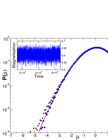
(a) Comparison at $T<T_{\mathrm{c}}$ and $H=0$

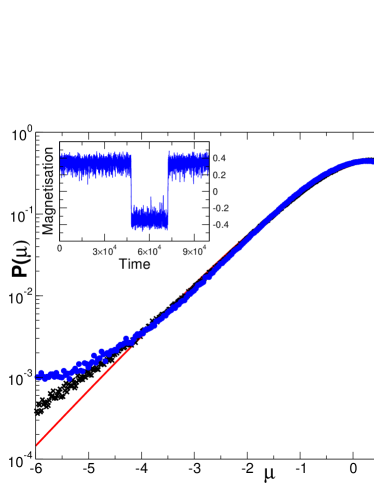
(b) Comparison at $T=T^{*}$ and $H=0$

Figure 1: Numerical test of the Langevin dynamics, for $\lambda=2.5$ and $L=65$. (a) The data ($\times$) are Monte Carlo simulations at $T=1.7$ and $L=64$.The data ($\bullet$) are obtained by Langevin dynamics from equation ( 4) at $T_{\mathrm{dyn}}=T_{\mathrm{c}}^{\mathrm{mf}}\times 0.74$. The plain curve corresponds to the distribution of the Gaussian model ($L=64$) with mass $M=3.5\times 10^{-1}$ [14]. (b) The plain curve is the BHP distribution [6]. The data ($\times$) are Monte Carlo simulations for $L=64$ system at $T^{*}(L)=T_{\mathrm{c}}\times 0.94$ [8]. The data ($\bullet$) are from the Langevin dynamics (4), at $T^{*}(L,\lambda)=T_{\mathrm{c}}^{\mathrm{mf}}\times 0.95$. Inset: examples of magnetization dynamics.

We have now all the ingredients to compute $P(m,\tau)$, the PDF of the instantaneous magnetization $m$ at time $\tau$. It is given by, $P(m,\tau)=\langle\delta\big{(}m-m_{\mathrm{tot}}(\tau)\big{)}\rangle_{\{\eta_{0},\eta_{{\bm{q}}}\}}.$ As previously [3, 6] we introduce a reduced scaling variable for the magnetization. Here we are interested in fluctuations around the typical value of $m$, $\bar{m}=\langle m_{\mathrm{tot}}\rangle_{\{\eta_{{\bm{q}}}\}}$, where the average is performed over all noise except $\eta_{0}$. Similarly we define the width of the distribution as $\bar{\sigma}^{2}=\langle m_{\mathrm{tot}}^{2}\rangle_{\{\eta_{{\bm{q}}}\}}-\bar{m}^{2}$, and the reduced magnetization $\mu_{\mathrm{tot}}=(m-\bar{m})/\bar{\sigma}$. We stress that $\bar{m}$ and $\bar{\sigma}^{2}$ are not the mean and variance of the instantaneous magnetization, as we have not averaged over the noise $\eta_{0}$.
At this stage of our derivation, it is useful to numerically check the approximations and assumptions made so far, i.e. the perturbation expansion, the Langevin dynamics and the logic of the separation of time scales. In figure 1(a) we show data generated by integrating numerically equations (4) for a temperature below the mean-field critical temperature, at zero field. This shows that perturbation theory can indeed capture the first departure from Gaussian fluctuations, as the critical point is approached. In figure 1(b) we compare the PDF obtained from Monte Carlo simulations at $T^{*}(L=64)=T_{\mathrm{c}}\times 0.94$ [8] with the results of Langevin dynamics at $T^{*}(L=65,\lambda=2.5)=T_{\mathrm{c}}^{\mathrm{mf}}\times 0.95$. As one can see the agreement is good and the data give an equally good fit to the BHP function. Differences appear in the wings of the distribution. The perturbation scheme overestimates the value of the PDF, illustrating the limit of its validity. However, it is clear that, at least in the case where the symmetry is effectively broken and where our criterion (2) is satisfied, the scheme captures the magnetic fluctuations of the Ising model to an excellent approximation. Our scheme has to be compare with mean-field treatment of Zheng [13] where a simple approximation or ansatz can also describe most of the features. Here however, the connection with the XY-model is revealed through a separation of the “fast” variables, described by spin waves like excitations, and “slow” variables, representing the evolution of the global magnetization within the effective potential minima.

3 Probability density function of the fluctuations

Using the integral representation of the Dirac function, $P(m,\tau)$ can be written as a path integral over the noise $\eta_{0}$ and $\eta_{\bm{q}}$. As the equations on $\phi_{\bm{q}}^{(\alpha)}$ are linear (4), they can be integrated out if we assume that $\phi_{0}$ is slowly varying with time. This is true at low temperature: $\phi_{0}$ is the instantaneous magnetization within the mean-field approximation, and the fluctuations around this value are represented by the $\phi_{\bm{q}}^{(\alpha)}$. The amplitude of the fluctuations of the global variable $\phi_{0}$ in equation (4) are scaled by the factor $1/N$ coming from ${\cal S}_{0}$, and therefore $\phi_{0}$ does not, at least at low temperature, venture far from the energy minima. In this case, the quantity $G_{{\bm{q}}}$, which depends on $\phi_{0}$, can be considered as constant. That is, we can replace the propagator by its time averaged value during the period $\tau$.
After some algebra, defining $g_{k}=2\sum_{{\bm{q}}\in S_{1}}\left[K_{\bm{q}}G_{\bm{q}}\coth(\tau/G_{\bm{q}})\right]^{k}/N^{k}$, one finally obtains

$$P(m,\tau)=\int\mathcal{D}\eta_{0}(t)\exp\left(-\frac{1}{4}\int_{0}^{\tau}\eta_{0}^{2}(u)\mathrm{d}u\right)\Pi_{XY}[\phi_{0}](\mu_{\mathrm{tot}},\tau),$$ (5)

$$\Pi_{\mathrm{XY}}[\phi_{0}](\mu_{\mathrm{tot}},\tau)=\int_{-\infty}^{+\infty}\frac{\mathrm{d}x}{2\pi\bar{\sigma}}\exp\left(ix\mu_{\mathrm{tot}}+\frac{1}{2}\sum_{k=2}^{\infty}\frac{g_{k}}{k}\left(\sqrt{\frac{2}{g_{2}}}ix\right)^{k}\right).$$

The function $\Pi_{\mathrm{XY}}$ is the PDF for the 2D-XY model in the spin wave approximation with a massive propagator, $G_{\bm{q}}^{-1}\varpropto q^{2}+M(\phi_{0})^{2}$ [14]. Here $\Pi_{\mathrm{XY}}$ depends on the temperature as the mass varies with temperature through $\phi_{0}$. In the limit $M\rightarrow 0$, the temperature dependence disappears and $\Pi_{\mathrm{XY}}$ becomes precisely the BHP function.
In order to obtain the PDF for $m_{\mathrm{tot}}$, we would have to evaluate the last path integral over $\eta_{0}$. This integral is related to the non linear Langevin equation (4). At $T=0$ the dominant solution of the equation of motion is $\phi_{0}^{(0)}(t)=\mathrm{constant}$, which is a solution of $\delta{\cal S}_{0}/\delta\phi_{0}(u)=0$: the mode $\phi_{0}^{(0)}$ does not have any dynamics and it affects the PDF only by imposing a finite mass $M(\phi_{0}^{(0)})$. Physically this means that the PDF for the Ising model at low temperature should be the same as that obtained for the 2D-XY model with a small magnetic field. This is exactly what we have observed in figure 1(a). At finite temperature however non constant solutions exist: these are the instantons associated with the non-linear Langevin equation (4). Expressing the path integral in (5) over $\eta_{0}(t)$ as a path integral over $\phi_{0}(t)$, using equation (4), it follows that the time dependent solutions extremize the integral $\int_{0}^{\tau}[\dot{\phi}_{0}(u)+\delta{\cal S}_{0}/\delta\phi_{0}(u)]^{2}\mathrm{d}u$. This leads to

$$P(m,\tau) = \int\mathcal{D}\phi_{0}(t)\exp\left[-\frac{1}{2}\big{(}{\cal S}_{0}[\phi_{0}(\tau)]-{\cal S}_{0}[\phi_{0}(0)]\big{)}\right]\times$$

$$\exp\left[-\frac{1}{4}\int_{0}^{\tau}\left(\dot{\phi}_{0}^{2}(u)+\left(\frac{\delta{\cal S}_{0}}{\delta\phi_{0}(u)}\right)^{2}-2\frac{\delta^{2}{\cal S}_{0}}{\delta\phi_{0}(u)^{2}}\right)\mathrm{d}u\right]\Pi_{\mathrm{XY}}[\phi_{0}](\mu_{\mathrm{tot}},\tau).$$

The second order derivative of ${\cal S}_{0}$, which comes from the Jacobian of the transformation, is of order $N$ compared with order $N^{2}$ for the other terms and is therefore negligible. To simplify the analysis, we assume periodic boundary conditions, $\phi_{0}(0)=\phi_{0}(\tau)$, and the first argument of the exponential in (3) vanishes. The non constant solutions $\phi_{0}^{(k)}(u)$, $k>1$ verify $\dot{\phi}_{0}(u)^{2}/2=V_{0}-V_{{\rm eff}}[\phi_{0}(u)]$, where $V_{0}>0$ is a constant of motion that depends on the instanton trajectory and $2V_{{\rm eff}}[\phi_{0}(u)]=-[\delta{\cal S}_{0}/\delta\phi_{0}(u)]^{2}$ is an effective inverted potential. From (3) we define an effective action $S_{{\rm eff}}$ whose $\phi_{0}^{(k)}$ are the classical time dependent solutions: $S_{{\rm eff}}[\phi_{0}(u)]=\int_{0}^{\tau}\left(\frac{1}{2}\dot{\phi}_{0}^{2}(u)-V_{{\rm eff}}[\phi_{0}(u)]\right)\mathrm{d}u$. Expressing $\mathrm{d}u$ as function of $\mathrm{d}\phi_{0}$, the constant $V_{0}$ satisfies the equation $\int\pm\frac{d\phi_{0}}{\sqrt{2(V_{0}-V_{{\rm eff}})}}=\tau.$ The sign is positive (resp. negative) when $\phi_{0}$ is increasing (resp. decreasing) with time. Generally, we assume that $V_{0}$ tends exponentially to zero when $\tau$ is large. For an action with two wells ${\cal S}_{0}=-a\phi_{0}^{2}/2+\phi_{0}^{4}/4$, with $a\propto T_{c}-T$, we can evaluate this constant. Indeed, if we consider a trajectory going from $\phi_{0}(0)=\sqrt{a}$ to $\phi_{0}=0$ at some later fixed time, then going back to $\sqrt{a}$ at time $\tau$, this corresponds to solving the following equation: $2\int_{0}^{\sqrt{a}}\frac{d\phi_{0}}{\sqrt{2(V_{0}-V_{{\rm eff}})}}=\tau$. When $\tau$ is large, $V_{0}$ has to be small, and the main contributions from the previous integral come from the end points: $V_{{\rm eff}}\simeq-2a^{2}(\phi_{0}\mp\sqrt{a})^{2}$ for $\phi_{0}$ close to $\pm\sqrt{a}$, and $V_{{\rm eff}}\simeq-a^{2}\phi_{0}^{2}/2$ for $\phi_{0}$ close to 0. It is then easy to show that $V_{0}\propto\exp(-\sqrt{2}a\tau)$ and it is hence legitimate to discard this constant for large time $\tau$. The effective action $S_{\mathrm{eff}}$ can be simplified in this case, and is equal to $\Delta{\cal S}_{0}^{(k)}$, the sum of the energy barriers crossed by the instanton $\phi_{0}^{(k)}$ during the time $\tau$. Finally, the distribution (3) can be put into the following form

$$P(m,\tau)\sim\Pi_{\mathrm{XY}}[\phi_{0}^{(0)}](\mu_{\mathrm{tot}})+\sum_{k\geq 1}C_{k}\exp\left(-\Delta{\cal S}_{0}^{(k)}\right)\Pi_{\mathrm{XY}}[\phi_{0}^{(k)}](\mu_{\mathrm{tot}},\tau),$$ (7)

where the $C_{k}$’s are coefficients related to the Gaussian fluctuations around the saddle point solutions $\phi_{0}^{(k)}$. These instantons restor the system symmetry. Below the critical region they appear only on exponentially large time scales, and can be neglected on the time scale of any observations. Near the critical point they appear more frequently and lead to a phase transition in the finite system. It is extremely challenging to exactly compute the contribution from the instantons [15] and to do so would, in any case, give only an approximate description of the true critical dynamics, so we do not attempt it here. Rather, the final expression (7) is sufficient for our purposes as it exposes both the origin of generic critical fluctuations and of the dependence on universality classes through the generation of instanton like excitations.

4 Interpretation and generalization

We have shown that at this level there are two distinct contributions to the PDF for magnetic fluctuations in equation (7). The first is a Gaussian action coming directly from the perturbation expansion and as long as quadratic fluctuations are present, such a term must appear. The limiting case of zero mass corresponds BHP distribution. The Ising model universality class does not appear in this term and in this sense it is superuniversal. The fluctuations described here are localized around the typical value of the magnetization and are sensitive to the local geometry around this point in phase space, not to the global structure of the phase space related to the universality class. The second term comes from the contribution of instantons that restore phase space symmetry and so is strongly dependent on the universality class. It is the analogue of the corrections computed exactly for the 2D-XY model within the spin wave approximation [9, 10]
The existence of a point, or points, in the phase diagram where the PDF of the 2D Ising model is close to the BHP distribution [8] results from a compromise between these two terms: to be as close as possible to BHP, we have to reduce the mass in the Gaussian propagators of the first term. This is exactly what happens as one approaches $T_{\mathrm{c}}$ and the instantaneous value of $\phi_{0}$ reduces. At the same time the contribution from instantons has to be small, which is not the case at $T_{\mathrm{c}}$: reducing $\phi_{0}$ increases the probability of inducing an instanton, taking the system from one local minimum to the other. This occurs just as the correlation length becomes of the order of the system size, hence the instanton contribution being small corresponds exactly to our criterion (2) being satisfied. The temperature $T^{*}$ studied in [8] is the point of best compromise. The application of a small magnetic field breaks the symmetry, increasing the barriers $\Delta{\cal S}_{0}^{(k)}$. The contribution from instantons is then reduced and one can expect better agreement with BHP than in zero field. This is just what is observed. However, while the agreement with BHP can be excellent it is approximate and there will always be corrections to it.

What other correlated systems show similar behaviour ? The previous analysis suggests that generic behaviour reminiscent of the D-dimensional Gaussian model should indeed be commonly observed in equilibrium correlated systems in D-dimensions. We show in fact that fluctuations of this generic type correspond to perturbative corrections to the central limit theorem and that in this sense such systems should be thought of as being weakly, rather than strongly correlated. It suggests also that one should expect variations. These variations can be large, coming from non-linear instanton-like objects, taking the distribution far from the generic asymmetric form shown in Fig.1(b) [8, 16], or they can be smaller, coming from the harmonic contribution itself. That is, the BHP function is not a miraculous unique function for all circumstances, rather distributions of the form of the first term in equation (7) depend weakly on the boundary conditions [6, 17, 18], on the mass [14] and even on the temperature [9, 10]. Of these parameters the strongest dependence is on dimension: we expect that 3D correlated equilibrium systems are related to the 3D Gaussian model, which has weakly asymmetric order parameter fluctuations and is not critical [6, 19]. Interestingly, out of equilibrium three dimensional systems show results resembling the 2D-XY model[1, 2, 4], or the closely related Gumbel distribution [17] characteristic of a one-dimensional system with long range interactions not those of the 3D-XY model. These results seem to suggest the presence of a dimensional reduction in such systems that remains to be explained.

- [1] S.T. Bramwell, P.C.W. Holdsworth and J.-Y. Pinton, Nature 396, 512 (1998)
- [2] S.T. Bramwell et al., Phys. Rev. Lett. 84, 3744 (2000)
- [3] R. Labbé, J.-F. Pinton, and S. Fauve, J. Phys. II (France) 6 1099 (1996)
- [4] T. Tóth-Katona and J. Gleeson, Phys. Rev. Lett. 91, 24501 (2003).
- [5] B. Ph. van Milligen et al., Phys. of Plasmas, 12, 052507 (2005).
- [6] S.T. Bramwell et al., Phys. Rev. E 63, 041106 (2001)
- [7] G. Palma, T. Meyer and R. Labbe, Phys. Rev. E 66, 026108 (2002)
- [8] M. Clusel, J.-Y. Fortin and P.C.W. Holdsworth, Phys. Rev. E 70, 046112 (2004)
- [9] S.T. Banks and S.T. Bramwell, J. Phys. A: Math. Gen. 38, 5603 (2005)
- [10] G. Mack, G. Palma and L. Vergara, Phys. Rev. E 72, 026119 (2005)
- [11] G. Parisi, Statistical Field Theory, Perseus press (1998)
- [12] N. Goldenfeld, Lectures on Phase Transitions and the Renormalisation group, Addison-Wesley (1992)
- [13] B. Zheng, Phys. Rev. E 67, 026114 (2003)
- [14] B. Portelli et al., Phys. Rev. E 64, 036111 (2001).
- [15] F.J. Alexander, S. Habib, and A. Kovner, Phys. Rev. E 48, 4284 (1993)
- [16] N. R. Moloney, Ph.D. Imperial College London, 2004.
- [17] T. Antal et al. Phys. Rev. Lett, 87, 240601, (2001). ibid Phys. Rev. E 65, 046140 (2002).
- [18] A. Rosso et al., Phys. Rev. E 68, 036128 (2003)
- [19] C. Chamon et al., J. Chem. Phys, 121, 10120 (2004)