Microscopic theory for interface fluctuations in binary liquid mixtures

Abstract

Thermally excited capillary waves at fluid interfaces in binary liquid mixtures exhibit simultaneously both density and composition fluctuations. Based on a density functional theory for inhomogeneous binary liquid mixtures we derive an effective wavelength dependent Hamiltonian for fluid interfaces in these systems beyond the standard capillary-wave model. Explicit expressions are obtained for the surface tension, the bending rigidities, and the coupling constants of compositional capillary waves in terms of the profiles of the two number densities characterizing the mixture. These results lead to predictions for grazing-incidence x-ray scattering experiments at such interfaces.

I Introduction

If two thermodynamically coexisting fluid phases are brought into spatial contact via suitable boundary conditions, an interface forms which interpolates smoothly between the bulk properties of the coexisting phases. For more than a hundred years substantial theoretical and experimental efforts have been devoted to resolve the structural properties of this transition region (see, e.g., Refs. Rowlinson and Widom (1982); Jasnow (1984)).
The reason for the persistence of these challenge resides in the difficulty to describe the simultaneous occurrence of bulk fluctuations reaching the interface and of capillary wave-like fluctuations of the local interface position Mecke and Dietrich (1999). For the simplest example, i.e., the liquid-vapor interface of a one-component fluid, the concept of an effective interface Hamiltonian leads to quantitative predictions for a wavelength-dependent surface tension Helfrich (1973); Blokhuis and Bedeaux (1991); Napiórkowski and Dietrich (1993); Blokhuis et al. (1999); Mecke and Dietrich (1999), which has been confirmed experimentally for the interface structure factor down to microscopic length scales for a wide variety of one-component fluids Fradin et al. (2000); Daillant et al. (2001); Mora et al. (2003); Li et al. (2004); Lin et al. (2005). For these systems the wavelength dependent surface tension $\gamma(q=2\pi/\lambda)$ is a function of temperature $T$ and a functional of the interaction pair potential of the fluids particles. The macroscopic surface tension $\gamma=\gamma(0)$ of the liquid-vapor interface is obtained for $q\rightarrow 0$ whereas $\gamma(q)$ decreases for increasing values of $q$, reaches a substantial minimum, and increases again for large $q$. This decrease of $\gamma(q)$ is in a accordance with simulation data Stecki (1998); Milchev and Binder (2002); Vink et al. (2005) which, however, have not yet confirmed the predicted and experimentally observed re-increase of $\gamma(q)$ at large $q$.
The present work aims at extending this analysis to the case of binary liquid mixtures composed of species $A$ and $B$. This is motivated by the following reasons:

1. Binary liquid mixtures are governed by three pair potentials $w_{ij}(\mathbf{r})$ for the $A$-$A$ and $B$-$B$ interaction between the like species and the $A$-$B$ interaction between unlike species. Provided a wavelength dependent surface tension can be introduced analogous to the one for one-component fluids, it will therefore be a functional of three pair potentials. By exchanging systematically one of the two components by a sequence of molecules with a quasi-continuously changing architecture, this might open the possibility to tune the shape of the function $\gamma(q)$ and thus to create new interfacial phenomena.

2. Whereas for one-component fluids two-phase coexistence is confined to a liquid-vapor coexistence line described by the chemical potential $\mu_{o}(T)$, in binary liquid mixtures two fluid phases can coexist on a two-dimensional sheet in their thermodynamic parameter space $(\mu_{A},\mu_{B},T)$ spanned by the chemical potentials $\mu_{A}$ and $\mu_{B}$ of the two species and temperature (see Fig. 1). This allows one to vary the thermodynamic state of the system over a considerably larger parameter space without loosing two-phase coexistence, which in turn increases the possibilities to vary $\gamma(q)$ by changing thermodynamic variables such as the composition.

3. Generically, for one-component systems liquid and vapor are the only fluid phases and thus liquid-vapor interfaces are the only possible fluid interfaces in such systems. Binary liquid mixtures exhibit various fluid phases: a mixed vapor phase, a mixed liquid phase, an $A$-rich liquid phase, and a $B$-rich liquid phase, separated from each other by sheets of first-order phase transitions which intersect along a triple line of three-phase coexistence and which are delimited each by lines of critical points (see, e.g., Refs. Dietrich and Latz (1989); Getta and Dietrich (1993); Dietrich and Schick (1997) and Fig. 1). Depending on the relative integrated strength of the attractive parts of the aforementioned three pair potentials, there is a wide range of rather different topologies of the bulk phase diagrams of binary liquid mixtures van Konynenburg and Scott (1980). These topologies of the bulk phase diagrams allow for four distinct types of fluid interfaces: vapor|mixed fluid, vapor|$A$-rich fluid, vapor|$B$-rich fluid, $A$-rich liquid|$B$-rich liquid. In contrast to one-component systems this offers the possibility to vary significant features of fluid interfaces without changing the underlying interaction potentials but only the thermodynamic state.

4. The description of inhomogeneous binary liquid mixtures requires two number density profiles, $\rho_{A}(z)$ and $\rho_{B}(z)$, where $z$ denotes the distance from the mean interface position along the $z$ axis. In many cases it is suitable to introduce instead the total number density $\rho(z)=\rho_{A}(z)+\rho_{B}(z)$ and the concentration $X(z)=\rho_{A}(z)-\rho_{B}(z)$ as linear combinations. Whereas for one-component systems it is straightforward (as in Ref. Mecke and Dietrich (1999)) to assign a local liquid-vapor interface position $f(x,y)$ to a given density configuration as the position of an isodensity surface (e.g., points $\mathbf{s}$ where $\rho(\mathbf{s})=(\rho_{liq}+\rho_{vap})/2$), such a construction is not clear from the outset in the presence of two fluctuating densities. Thus, the study of fluid interfaces in binary liquid mixtures raises the challenging conceptual issue how and to which extent they can be described microscopically in terms of an effective Hamiltonian $\mathcal{H}[f]$ and a wavelength dependent surface tension $\gamma(q)$.

5. It requires special care to prepare a bona fide one-component fluid. Naturally, systems come as multicomponent samples. Generally, segregation phenomena occur at their interfaces, which might influence significantly the interface fluctuations and vice versa. By choosing suitable series of molecules of related architecture and appropriate concentrations, binary fluid mixtures offer the possibility to interpolate systematically between the material properties of the corresponding limiting one-component systems, which generates substantial application perspectives. Finally, binary liquid mixtures can serve as rudimentary polydisperse systems as they occur in colloid suspensions. The study of interfacial properties in such systems has become very rewarding because they can be analyzed in great detail by direct optical techniques Aarts et al. (2004a, b), allowing for quantitative comparisons with theoretical predictions on the scale of the particles.

As mentioned above, two types of fluctuations occur simultaneously at interfaces: (a) fluctuations of the density as they occur in the bulk on length scales up to the bulk correlation length $\xi$; (b) in the absence of gravity and for large system sizes the mean position of the interface can be shifted without cost of free energy. This gives rise to thermally excited Goldstone modes leading to lateral fluctuations of the local interface position, with wavelengths reaching macroscopic values. Depending on which type of fluctuation is emphasized, originally two different approaches for the theoretical understanding have emerged.

As put forward by van der Waals van der Waals (1894), the first approach leads to a so-called intrinsic density profile which interpolates smoothly between the constant densities in the coexisting bulk phases. The interface is laterally flat and is kept in place by boundary conditions or a small gravitational field acting along the interface normal. The width of the intrinsic profile Jasnow (1984); Weeks (1977); Bedeaux and Weeks (1985) is given by the bulk correlation length, which diverges upon approaching the critical point $T_{c}$ of the corresponding two-phase coexistence, reflecting the disappearance of the interface at $T_{c}$. Accordingly, the van der Waals picture is expected to capture the interfacial properties at elevated temperatures close to $T_{c}$.

The second approach, conceived by Buff, Lovett, and Stillinger Buff et al. (1965), describes the width of an interface as a result of capillary-wave like fluctuations of a step-like intrinsic density profile. Here only the local interface positions are the statistical variables. The resulting mean density profile attains the bulk values like a Gaussian whereas the van der Waals approach yields an exponential decay for short-ranged forces between the fluid particles or inverse power laws in the presence of dispersion forces Dietrich and Napiórkowski (1991b). Within the capillary-wave model the width of the mean interface diverges upon switching off gravity or increasing the lateral system size. This roughening effect is missed by all available van der Waals approaches. On the other hand the capillary wave model misses the fact that the interfacial width diverges upon approaching $T_{c}$ on the scale of the bulk correlation length $\xi$.

Accordingly one can state that the van der Waals approach captures fluctuations on the length scale of $\xi$ and below and is suitable at high temperatures whereas the capillary wave approach is valid at low temperatures and captures the fluctuations with wavelengths larger than $\xi$. In Ref. Mecke and Dietrich (1999) these two approaches have been reconciled by considering intrinsic density profiles, as obtained from density functional theory, which undergo fluctuations of their lateral positions. Density functional theory provides expressions for the cost in free energy of such density configurations relative to the free energy of a flat interface. This yields an effective interface Hamiltonian $\mathcal{H}[f]$ and thus provides the statistical weight of interfacial fluctuations $f$. This statistical weight can also be used to calculate correlations of the local interface normals Mecke and Dietrich (2005); Aarts et al. (2005).

Inspired by the motivation described above, the present work extends the concept of Ref. Mecke and Dietrich (1999) to the description of fluid interfaces of binary liquid mixtures. After a brief discussion of the bulk phase diagrams of binary liquid mixtures (Subsec. II.1) we introduce the density functional theory which we use as the starting point for the description of spatially inhomogeneous fluids (Subsec. II.2). We define the effective interface Hamiltonian $\mathcal{H}$ for mixtures in Subsec. II.3. After discussing the crude approximation of steplike density profiles (Subsec. II.4), in Subsec. II.5 we introduce the central approximation which we actually use for further calculations. It involves the influence of the curvatures of the iso-density contours on the density profiles which has turned out to be crucial in order to describe the fluctuations of a liquid-vapor interface (see Ref. Mecke and Dietrich (1999)). Since this approach cannot simply be transferred to binary liquid mixtures requiring two iso-density contours, Sec. II is closed by remarks about how to overcome these additional problems. In Subsec. II.6 and Appendices A and B we present the explicit expressions for the effective interface Hamiltonian $\mathcal{H}$ based on the above-mentioned approximations. In order to be able to make predictions for scattering experiments from such interfaces, in Sec. III we present a Gaussian approximation of the effective interface Hamiltonian $\mathcal{H}$ using various representations and we discuss the resulting contributions (Subsecs. III.1-C). In Sec. IV we analyze the temperature and the composition dependence of structural properties of interfaces in binary liquid mixtures as inferred from the correlation functions. We summarize our results in Sec. V.

II Effective Interface Hamiltonian

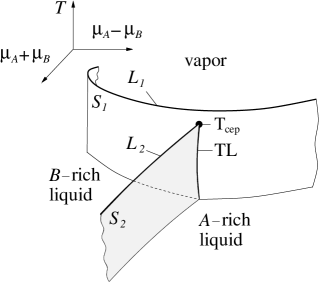
Fig. 1: Schematic bulk phase diagram of a binary liquid mixture in the thermodynamic parameter space $(\mu_{A}+\mu_{B},\mu_{A}-\mu_{B},T)$ spanned by the chemical potentials $\mu_{A}$ and $\mu_{B}$ of the two species and temperature $T$. As mentioned in the introduction, the phase diagram exhibits a vapor phase, a mixed liquid phase, an $A$-rich liquid phase, and a $B$-rich liquid phase separated by sheets $S_{1}$ and $S_{2}$ of first order-phase transitions which are bounded by lines $L_{1}$ and $L_{2}$, respectively, of second-order phase transitions. The line of intersection between $S_{1}$ and $S_{2}$ represents the triple line TL where three phases coexist. $\mathrm{T}_{\mathrm{cep}}$ denotes the critical end point. In the present context of fluid interfaces the solid phases of a binary liquid mixture, which occur at high pressures $(\sim\mu_{A}+\mu_{B})$ or low temperatures, are omitted for reasons of simplicity. Further details can be found in Refs. Dietrich and Latz (1989); Getta and Dietrich (1993); Dietrich and Schick (1997).

In this section we derive an effective interface Hamiltonian $\mathcal{H}$ for the interface between two fluid phases of a simple binary liquid mixture consisting of spherical particles with radially symmetric interaction potentials. The system with its interface is described microscopically in terms of a simple, but for the present purpose appropriate grand canonical density functional. For each of the two equilibrium particle density distributions we specify implicitly an iso-density contour as its interface surface assuming that this captures the interface structure of the mixture as a whole. The interface effective Hamiltonian, which counts the cost in free energy to deform the interfaces from a given reference configuration, is defined as the difference between two grand canonical potentials corresponding to two different surface configurations. Further simplifications are made to express this Hamiltonian explicitly, rather in terms of the surfaces, in terms of the yet unknown, inhomogeneous densities. Thus, by construction, the microscopic interactions between the particles are taken into account transparently, which finally lead to effective interactions between the surfaces. To a large extent the functional dependence on the interaction potentials is kept general. Ultimately, for numerical evaluations, we assume long-ranged attractive dispersion forces.

The normal of the mean interface of the binary liquid mixture is taken to be oriented along the $z$-axis such that, for instance, the liquid phase and the vapor phase of the mixture are approached for $z\rightarrow-L$ and $z\rightarrow+L$, respectively (see Fig. 2). Density functional theory assigns a free energy to each density configuration such that the equilibrium configuration minimizes the functional and yields the corresponding grand canonical potential. As the natural reference configuration we choose what we call the flat state, in which the iso-density contours are laterally constant surfaces and do not vary with $\mathbf{R}=(x,y)$ (see Fig. 2). If present, gravity points into the negative $z$-direction.

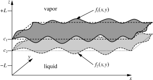
Fig. 2: Sketch of the liquid-vapor interface region of a binary liquid mixture with its normal oriented along the $z$-axis; for each of the two fluctuating densities of the mixture an interface position can be defined (dark and light grey, see the main text, and Eqs. (4) and (5)). In order to derive the interface Hamiltonian, two interface configurations are considered: the reference surface configuration is given by constant iso-density contours for the two species $A$ and $B$ at $z=c_{1}$ and $z=c_{2}$, respectively, while a non-flat configuration with iso-density contours $z=f_{1}(x,y)$ and $z=f_{2}(x,y)$ varies laterally around the position $c_{1}$ and $c_{2}$, respectively, so that $\langle f_{1}\rangle=c_{1}$ and $\langle f_{2}\rangle=c_{2}$. Additionally, the non-flat surfaces are assumed to fluctuate mildly without overhangs or bubbles, so that a Monge representation with $f_{i}(x,y)$, $i\in\{1,2\}$, can be used. Vapor and liquid should be understood as representations of two fluid phases including a mixed liquid, an $A$-rich liquid, and a $B$-rich liquid (see Subsec. II.1).

II.1 Bulk phase diagram of binary liquid mixtures

As stated in the introduction, binary liquid mixtures are composed of two species, called $A$ and $B$ particles. At high temperatures these particles mix in a gaseous phase. Upon lowering the temperature the mixture exhibits a phase separation into a gas phase of low density and a liquid phase of high density. In Fig. 1 this phase separation is indicated by the sheet $S_{1}$ with $\mu_{A}+\mu_{B}$ as a measure of the total pressure of the system. At sufficiently high temperatures in both these phases the two species remain mixed. A further decrease of the temperature leads to an additional phase separation of the fluid phase into an $A$-rich liquid phase and a $B$-rich liquid phase (see sheet $S_{2}$ in Fig. 1). In the following any pair of the mixed gas, mixed fluid, $A$-rich liquid, and $B$-rich liquid are denoted as liquid and vapor. Their coexistence corresponds to a point on $S_{1}$ or $S_{2}$ and, for instance, an increase of temperature at coexistence delineates a path on $S_{1}$ or $S_{2}$ approaching the line of critical points $L_{1}$ or $L_{2}$, respectively. On the other hand, changing the composition of the mixture at a fixed temperature at coexistence corresponds to a path on $S_{1}$ or $S_{2}$ intersecting a horizontal $(\mu_{A}+\mu_{B},\mu_{A}-\mu_{B})$-plane in Fig. 1. In Sec. IV we shall discuss our results in two respects: first, we study the influence of temperature and, second, we shall keep the temperature fixed and consider composition variations.

II.2 Density Functional Theory

We consider a grand canonical density functional for a two-component fluid which consists of particles $A$ and $B$ with a spherically symmetric interaction potentials $W_{ij}(|\mathbf{r}|)=W_{ji}(|\mathbf{r}|)$, where the indices $i,j\in\{1,\,2\}$ refer to the species $A$ and $B$. Following standard procedure Evans (1979) the interaction potential is split into a short-ranged repulsive part $s_{ij}(r)$ and an attractive long-ranged part $w_{ij}(r)$. For a system of volume $V=2L\,A$, where $A$ is the (flat) interfacial area and $2L$ is the macroscopically large extension in $z$ direction, a simple version of the grand canonical density functional $\Omega$ reads:

$$\Omega[\rho_{1}(\mathbf{r}),\rho_{2}(\mathbf{r})] = \;\mathcal{F}^{\mathsf{hs}}[\rho_{1}(\mathbf{r}),\rho_{2}(\mathbf{r})]$$ (1)

$$+\,\sum_{i=1}^{2}\int_{V}\!d^{3}r\;\big{(}\mu_{i}+V_{i}^{\mathsf{ex}}(\mathbf{r})\big{)}\rho_{i}(\mathbf{r})$$

$$+\,\frac{1}{2}\sum_{i,j=1}^{2}\,\int_{V}\!d^{3}r\!\int_{V}\!d^{3}r^{\prime}\;\;w_{ij}(|\mathbf{r}-\mathbf{r}|)\rho_{i}(\mathbf{r})\rho_{j}(\mathbf{r}^{\prime})\,.$$

Here, $\rho_{i}(\mathbf{r})$ is the number density of the particles of species $i\in\{1,2\}$ at $\mathbf{r}=(x,y,z)=(\mathbf{R},z)$, and $\mathcal{F}^{\mathsf{hs}}[\rho_{1}(\mathbf{r}),\rho_{2}(\mathbf{r})]$ is the reference free energy functional of a system governed by the short-ranged contribution $s_{ij}(|\mathbf{r}|)$, expressed suitably in terms of a hard-sphere system. In the following, we use $\mathcal{F}^{\mathsf{hs}}[\rho_{1}(\mathbf{r}),\rho_{2}(\mathbf{r})]$ within a local density approximation:

$$\mathcal{F}^{\mathsf{hs}}[\rho_{1}(\mathbf{r}),\rho_{2}(\mathbf{r})]=\int_{V}\!d^{3}r\;h\big{(}\rho_{1}(\mathbf{r}),\rho_{2}(\mathbf{r})\big{)}\,.$$ (2)

In Eq. (1) the chemical potential of species $i$ is denoted by $\mu_{i}$, while $V_{i}^{\mathsf{ex}}(\mathbf{r})$ represents its external potential, which in our case will be gravity acting along the negative $z$-axis. The attractive part of the pair interactions is given by $w_{ij}(|\mathbf{r}|)\equiv w_{ij}(r)$. To a large extend our reasoning will not depend on specific choices for $h\big{(}\rho_{1}(\mathbf{r}),\rho_{2}(\mathbf{r})\big{)}$, $V_{i}^{\mathsf{ex}}$, and $w_{ij}(r)$. This will be required only for quantitative presentations. Actually $w_{ij}(r)$ should be replaced by the direct correlation function $c_{ij}^{(2)}(r)$ which, however, reduces to $w_{ij}(r)$ for large $r$. This replacement also does not alter our main results.
With the notation $\mathbf{R}=(x,y)$ we introduce the bulk densities

$$\rho_{i}^{\pm}:=\rho_{i}(\mathbf{R},z\rightarrow\pm L)\,,\;i\in\{1,2\}\,$$ (3)

characterizing the vapor ($\rho_{i}^{+}$) and the liquid phase ($\rho_{i}^{-}$) in the general sense described above. In order to describe density configurations as shown in Fig. 2 we introduce $\rho_{c_{i}}(z)$ and $\rho_{f_{i}}(\mathbf{r})$ as the density profiles of species $i$ which take a fixed value $\bar{\rho}_{i}$ at the position $z=c_{i}$ for a flat configuration and at $z=f_{i}(\mathbf{R})$ for a non-flat configurations, respectively. For the non-flat iso-density surfaces we assume a Monge parameterization (see Fig. 2). Thus, the crossing criterions are

$$\rho_{c_{i}}(z=c_{i}) = \bar{\rho}_{i}$$ (4)

and

$$\rho_{f_{i}}(\mathbf{R},z=f_{i}(\mathbf{R})) = \bar{\rho}_{i}\,.$$ (5)

The indices $c_{i}$ and $f_{i}$ indicate that these functions of $z$ only and of $\mathbf{r}=(\mathbf{R},z)$ take the constant value $\bar{\rho}_{i}$ at $z=c_{i}$ and at $z=f_{i}(\mathbf{R})$, respectively. Reasonable choices for $\bar{\rho}_{i}$ would be $\bar{\rho}_{i}:=(\rho_{i}^{-}+\rho_{i}^{+})/2$ or the analogue of the Gibbs dividing surface concept in the one-component fluids (see also Fig. 3); however, our results do not depend explicitly on the choices of $\bar{\rho}_{i}$. Finally we introduce the density differences

$$\triangle\rho_{i}:=\rho_{i}^{-}-\rho_{i}^{+}\,.$$ (6)

In the following we choose $\rho_{c_{i}}(z)$ and $\rho_{f_{i}}(\mathbf{r})$ such that they minimize Eq. (1) under the constraint given by Eq. (4) and Eq. (5), respectively:

$$\Bigg{(}\frac{\delta\Omega[\rho_{1}(\mathbf{r}),\rho_{2}(\mathbf{r})]}{\delta\rho_{i}(\mathbf{r})}\Bigg{)}_{c,f}=0\,,\;i\in\{1,2\}\,,$$ (7)

where $\Big{(}\delta\Omega[\rho_{1},\rho_{2}]/\delta\rho_{i}(\mathbf{r})\Big{)}_{c,f}$ denotes the functional derivative of $\Omega$ w.r.t the density $\rho_{i}$, under the constraint $c$ (see Eq. (4)) or $f$ (see Eq. (5)), respectively.
Within density functional theory, $\rho_{c_{i}}(z)$ and $\rho_{f_{i}}(\mathbf{r})$ are equilibrium density profiles in the sense described before. Inter alia, Eq. (7) will allow us to eliminate the explicit dependences on the chemical potentials $\mu_{i}$ in our analytic expressions; for this purpose it is sufficient to use Eq. (7) only for the profiles $\rho_{c_{i}}(z)$. Without constraint Eqs. (1) and (2) lead to

$$\frac{\delta\Omega[\rho_{1}(\mathbf{r}),\rho_{2}(\mathbf{r})]}{\delta\rho_{i}(\mathbf{r})} = \partial_{\rho_{i}}h\big{(}\rho_{1}(\mathbf{r}),\rho_{2}(\mathbf{r})\big{)}+\mu_{i}+V_{i}^{\mathsf{ex}}(\mathbf{r})$$ (8)

$$+\,\sum_{j=1}^{2}\int_{V}\!d^{3}\!s\;\;w_{ji}\big{(}|\mathbf{r}-\mathbf{s}|\big{)}\rho_{j}(\mathbf{s})\,.$$

Up to here there is no construction scheme provided for determining $\rho_{c_{1}}$ and $\rho_{c_{2}}$. One can take solutions of Eq. (8) for $V_{i}^{\mathsf{ex}}\equiv 0$ and shift the pair such that, e.g., the condition $\rho_{c_{1}}(z=c_{1})=\bar{\rho}_{1}$ is fulfilled (see Eq. (4)), but in general $\rho_{c_{2}}(z)$ will not have the property $\rho_{c_{2}}(z=c_{2})=\bar{\rho}_{2}$. This shows that there is only one degree of freedom in shifting, i.e., $c_{1}-c_{2}$. Thus, $c_{2}$ is not a free parameter but depends on $c_{1}$, which means that $\Omega$ cannot be minimized for arbitrary pairs $(c_{1},c_{2})$. As a consequence the effective interface Hamiltonian $\mathcal{H}$ depends only on the difference $c_{1}-c_{2}$, but we shall treat $c_{2}$ formally as a free parameter, which indicates the position of the planar interface of $\rho_{c_{2}}(z)$.

The free energy density $h\big{(}\rho_{1},\rho_{2}\big{)}=h^{\mathsf{id}}\big{(}\rho_{1},\rho_{2}\big{)}+h^{\mathsf{ex}}\big{(}\rho_{1},\rho_{2}\big{)}$ of the hard sphere part consists of an ideal gas contribution $h^{\mathsf{id}}\big{(}\rho_{1},\rho_{2}\big{)}$ and an excess part $h^{\mathsf{ex}}\big{(}\rho_{1},\rho_{2}\big{)}$. Our analytical formulae derived below will not depend on its functional form; for numerical calculations, however, the Carnahan-Starling expression $h^{\mathsf{CS}}\big{(}\rho_{1},\rho_{2}\big{)}$ for the excess contribution is used Carnahan and Starling (1969). With ($\beta=(k_{B}T)^{-1}$ and the thermal de Broglie wavelength $\lambda_{\mathsf{th}}$, this means

$$h^{\mathsf{id}}(\rho_{1},\rho_{2})=\beta^{-1}\,\sum_{i=1}^{2}\rho_{i}\,\big{(}\ln(\lambda_{\mathsf{th},i}^{3}\,\rho_{i})-1\big{)}$$ (9)

and

$$h^{\mathsf{CS}}(\rho_{1},\rho_{2}) = -\,n_{o}\,\ln\big{(}1-n_{3}\big{)}+\frac{n_{1}\,n_{2}}{1-n_{3}}$$ (10)

$$+\,n_{2}^{3}\;\frac{n_{3}+(1-n_{3})^{2}\,\ln\big{(}1-n_{3}\big{)}}{36\pi n_{3}^{2}(1-n_{3})^{2}}\,,$$

where

$$\begin{array}[]{ccc}n_{o}&=&\displaystyle{\sum_{k=1}^{2}\rho_{k}}\\ \\ n_{2}&=&\displaystyle{4\pi\sum_{k=1}^{2}\big{(}r_{o}^{(k)}\big{)}^{2}\rho_{k}}\end{array} \begin{array}[]{ccc}n_{1}&=&\displaystyle{\sum_{k=1}^{2}r_{o}^{(k)}\rho_{k}}\\ \\ n_{3}&=&\displaystyle{\frac{4\pi}{3}\sum_{k=1}^{2}\big{(}r_{o}^{(k)}\big{)}^{3}\rho_{k}}\,.\end{array}$$ (17)

The weighted densities $n_{\alpha}$, $\alpha\in\{0,1,2,3\}$, are composed of the densities $\rho_{i}$ and the particle radii $r_{o}^{(i)}$ of species $i\in\{1,2\}$.
In order to model the van der Waals forces of simple fluids we take for the attractive part of the interactions

$$w_{ij}(R,z)=-\frac{w_{o}^{(ij)}\,(r_{o}^{(ij)})^{6}}{\big{(}(r_{o}^{(ij)})^{2}+R^{2}+z^{2}\big{)}^{3}}\,,\;i,j\in\{1,2\}\;,$$ (18)

which gives the correct large distance behavior $w_{ij}(r\gg r_{o}^{(ij)})=-\,w_{o}^{(ij)}r^{-6}$. The quantity $w_{o}^{(ij)}$ represents the depth of the potential, while $r_{o}^{(ij)}=r_{o}^{(i)}+r_{o}^{(j)}$ is defined as the sum of the particle radii. The functional form of $w_{ij}(r)$ for small $r$ is chosen for analytic convenience; most of our results do not depend on this choice.

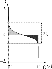
Fig. 3: Sketch of the planar number density profile $\rho_{c}(z)$; the width $2\xi=\xi^{+}+\xi^{-}$ of the transition region is roughly the sum of the bulk correlation lengths $\xi^{+}$ and $\xi^{-}$ of the two coexisting phases which, in general, differ from each other (see also the remarks related to, c.f., Eq. (64)). The length $\xi$ is also called the interfacial width of the (planar) surface located at $z=c$ (see Eq. (4)). The marked regions are frequently used to define the interface position via Gibbs’ zero-adsorption criterion: the number of particles within the dark and the light domain has to be the same for the interface at $z=c$ Rowlinson and Widom (1982). Within the sharp kink approximation one has $\xi=0$ so that a step-like profile results (see Eq. (34)).

Independent of the explicit form of the potentials $w_{ij}$ we introduce their integrals

$$w_{ij}^{(1)}(|\mathbf{R}|,z) := \int_{\delta c_{ij}}^{z}\!d\bar{z}\,\,w_{ij}(|\mathbf{R}|,|\bar{z}|)\hskip 28.45274pt$$ (19)

and

$$w_{ij}^{(2)}(|\mathbf{R}|,z) := \int_{\delta c_{ij}}^{z}\!d\bar{z}\,\,w_{ij}^{(1)}(|\mathbf{R}|,|\bar{z}|)$$ (20)

where $\delta c_{ij}:=c_{i}-c_{j}$. They fulfill the symmetry relations

$$w_{ij}^{(k)}(|\mathbf{R}|,z)=(-1)^{k}w_{ji}^{(k)}(|\mathbf{R}|,-z)\,,\;k\in\{1,2\}\,.$$ (21)

In the present context the binary liquid mixture is exposed to a gravitational field acting along the $z$ direction:

$$V_{i}^{\mathsf{ex}}(z) = G\,m_{i}\,(z-c_{i})\,,$$ (22)

where $G$ is the acceleration of gravity, $m_{i}$ is the particle mass and $c_{i}$ the equilibrium flat interface position of species $i$ (see Eq. (4)). In the following the first integral of $V_{i}^{\mathsf{ex}}(z)$ is frequently used:

$$V_{i}^{(1)}(z) := \frac{1}{2}\,G\,m_{i}\,(z-c_{i})^{2}\,.$$ (23)

In the following subsection the effective interface Hamiltonian will be defined on the basis of the density functional $\Omega$ introduced above.

II.3 Effective Interface Hamiltonian

The envisaged effective interface Hamiltonian $\mathcal{H}$ for a binary liquid mixture provides the cost in free energy to maintain interface configurations described by the iso-density contours $f_{i}(\mathbf{R})$, $i\in{1,2}$, relative to flat configurations $\rho_{c_{i}}(z)$. We expect that $\mathcal{H}$ depends on the differences $f_{i}^{c}(\mathbf{R}):=f_{i}(\mathbf{R})-c_{i}$. Therefore, we introduce the abbreviations

$$\mathbf{f}(\mathbf{R},\mathbf{R}^{\prime}) := \left(\begin{array}[]{c}f_{1}^{c}(\mathbf{R})\\ f_{2}^{c}(\mathbf{R}^{\prime})\end{array}\right)\,,$$ (26)

$\mathbf{f}(\mathbf{R}):=\mathbf{f}(\mathbf{R},\mathbf{R})$, $\delta f_{ij}^{c}(\mathbf{R},\mathbf{R}^{\prime}):=f_{i}^{c}(\mathbf{R})-f_{j}^{c}(\mathbf{R}^{\prime})$, $\delta f_{ij}(\mathbf{R},\mathbf{R}^{\prime}):=f_{i}(\mathbf{R})-f_{j}(\mathbf{R}^{\prime})$, and $\delta f_{ij}(\mathbf{R}):=f_{i}(\mathbf{R})-f_{j}(\mathbf{R})$. In terms of these quantities, the effective interface Hamiltonian $\mathcal{H}$ is defined as the difference of the corresponding grand canonical potentials:

$$\mathcal{H}[\mathbf{f}(\mathbf{R},\mathbf{R}^{\prime})]:=\Omega[\rho_{f_{1}}(\mathbf{r}),\rho_{f_{2}}(\mathbf{r}^{\prime})]-\Omega[\rho_{c_{1}}(z),\rho_{c_{2}}(z^{\prime})]\,.$$ (27)

Our main goal is to derive an explicit expression of $\mathcal{H}$ in terms of $f_{i}^{c}(\mathbf{R})$.
We rewrite $\mathcal{H}$ by carrying out partial integrations such that $\mathcal{H}$ is expressed mostly in terms of derivatives of profiles which are mainly confined to the interfacial region and vanish for $z\rightarrow\pm L$. Due to Eq. (3) one has $|f_{i}^{c}(\mathbf{R})|\ll L$ for all $\mathbf{R}$, i.e., the interface deviations are much smaller than the sample size. According to the structure of $\Omega$ in Eq. (1), $\mathcal{H}$ is the sum of four terms. The first term, which we shall treat later in Subsec. II.6 is given directly as

$$\mathcal{H}_{h}\big{(}\mathbf{f}(\mathbf{R})\big{)}:=\int_{-L}^{L}\!\!dz\,\Big{[}h\big{(}\rho_{f_{1}}(\mathbf{r}),\rho_{f_{2}}(\mathbf{r})\big{)}-h\big{(}\rho_{c_{1}}(z),\rho_{c_{2}}(z)\big{)}\Big{]}\,.$$ (28)

The second expression stems from the external potential $V_{i}^{\mathsf{ex}}(z)$ and has the form

$$\mathcal{H}_{V}\big{(}\mathbf{f}(\mathbf{R})\big{)}:=-\sum_{i=1}^{2}\int_{-L}^{L}\!\!dz\,V_{i}^{(1)}(z)\,\big{[}\partial_{z}\rho_{f_{i}}(\mathbf{r})-\partial_{z}\rho_{c_{i}}(z)\big{]}\,.$$ (29)

The third contribution involves the chemical potentials $\mu_{i}$ and additional boundary contributions which arise from the interaction potentials. With the constants

$$K_{k} := \mu_{k}+4\pi\sum_{j=1}^{2}\,\,\int_{A}\!\!d^{2}R\,\big{[}\bar{\rho}_{j}\,w_{jk}^{(1)}(|\mathbf{R}|,z=L)$$ (30)

$$\hskip 65.44133pt-\rho_{j}^{-}\,w_{jk}^{(1)}(|\mathbf{R}|,z=0)\big{]}$$

it reads

$$\mathcal{H}_{b}\big{(}\mathbf{f}(\mathbf{R})\big{)}:=-\sum_{i=1}^{2}\,K_{i}\,\int_{-L}^{L}\!\!dz\,(z-c_{i})\,\big{[}\partial_{z}\rho_{f_{i}}(\mathbf{r})-\partial_{z}\rho_{c_{i}}(z)\big{]}\,.$$ (31)

Finally, the contribution to $\mathcal{H}$ due to the attractive part of the interactions can be expressed as

$$\mathcal{H}_{w}\big{(}\mathbf{f}(\mathbf{R},\mathbf{R}^{\prime})\big{)} := -\frac{1}{2}\sum_{i,\,j=1}^{2}\int_{-L}^{L}\!\!dz\!\int_{-L}^{L}\!\!dz^{\prime}\;w_{ij}^{(2)}(|\delta\mathbf{R}|,\delta z)\times$$ (32)

$$\times\Big{[}\partial_{z}\rho_{f_{i}}(\mathbf{r})\,\partial_{z^{\prime}}\rho_{f_{j}}(\mathbf{r}^{\prime})-\partial_{z}\rho_{c_{i}}(z)\,\partial_{z^{\prime}}\rho_{c_{j}}(z^{\prime})\Big{]}\,$$

where $\delta\mathbf{R}:=\mathbf{R}-\mathbf{R}^{\prime}$ and $\delta z:=z-z^{\prime}$. Thus, Eqs. (27)-(32) lead to

$$\mathcal{H}[\mathbf{f}(\mathbf{R})] = \int_{A}\!\!d^{2}R\,\Big{[}\mathcal{H}_{h}\big{(}\mathbf{f}(\mathbf{R})\big{)}+\mathcal{H}_{b}\big{(}\mathbf{f}(\mathbf{R})\big{)}+\mathcal{H}_{V}\big{(}\mathbf{f}(\mathbf{R})\big{)}\Big{]}$$ (33)

$$+\,\int\!\!\!\!\int_{A}\!d^{2}R\,d^{2}R^{\prime}\;\;\mathcal{H}_{w}\big{(}\mathbf{f}(\mathbf{R},\mathbf{R}^{\prime})\big{)}\,.$$

In the following two subsections we analyze two different models for the profiles $\rho_{c_{i}}(z)$ and $\rho_{f_{i}}(\mathbf{r})$ in order to obtain analytic results for $\mathcal{H}$. The first approach assumes that at the interface position the densities vary discontinuously between the corresponding bulk values. This so-called sharp kink approximation will be discussed in Subsec. II.4. The second approach (Subsec. II.5) is based on continuous density profiles and takes the influence of the curvature of the iso-density contours on the densities into account.
The validity of our approach is also based on the assumption that in the thermodynamic limit, i.e., $A\rightarrow\infty$, all lateral boundary contributions to $\mathcal{H}$ vanish in Eq. (33).

II.4 Sharp Kink Approximation

The sharp kink approximation replaces the actual smooth variations of the density profiles (see Fig. 3) on the scale of the bulk correlation length by step functions:

$$\rho_{f_{i}}(\mathbf{r}) := -\triangle\rho_{i}\,\Theta(z-f_{i}(\mathbf{R}))+\rho_{i}^{-}$$ (34)

where $\Theta(x)$ is the Heaviside function so that

$$\partial_{z}\rho_{f_{i}}(\mathbf{r}) = -\triangle\rho_{i}\,\delta(z-f_{i}(\mathbf{R}))\,.$$ (35)

Similar expressions hold for $\rho_{c_{i}}(z)$ with $f_{i}(\mathbf{R})$ replaced by $c_{i}$. For one-component fluids this approximation has turned out to be surprisingly successful in describing liquid-vapor interfaces Napiórkowski and Dietrich (1993) and wetting phenomena Dietrich and Napiórkowski (1991b). From Eqs. (33) and Eq. (35) together with the expansion (see Eqs. (20), (21), and (26))

$$w_{ij}^{(2)}(|\delta\mathbf{R}|,\delta f_{ij}(\mathbf{R},\mathbf{R}^{\prime}))\approx\frac{1}{2}\,w_{ij}(|\delta\mathbf{R}|,\delta c_{ij})\,\left[\delta f_{ij}^{c}(\mathbf{R},\mathbf{R}^{\prime})\right]^{2}$$ (36)

we find

$$\mathcal{H}^{\mathsf{sk}}[\mathbf{f}(\mathbf{R},\mathbf{R}^{\prime})]$$ (37)

$$\approx \int_{A}\!\!d^{2}R\,\,\sum_{i=1}^{2}\triangle\rho_{i}\,\bigg{[}\frac{G}{2}\,m_{i}\,\left[f_{i}^{c}(\mathbf{R})\right]^{2}+\,f_{i}(\mathbf{R})\,\times$$

$$\times\Big{(}\partial_{\rho_{i}}h\big{(}\rho_{f_{1}},\rho_{f_{2}}\big{)}\Big{|}_{z=f_{i}(\mathbf{R})}-\partial_{\rho_{i}}h\big{(}\rho_{c_{1}},\rho_{c_{2}}\big{)}\Big{|}_{z=c_{i}}\Big{)}\,\bigg{]}$$

$$-\,\int\!\!\!\!\int_{A}\!d^{2}R\,d^{2}R^{\prime}\,\sum_{i,j=1}^{2}\frac{\triangle\rho_{i}\,\triangle\rho_{j}}{4}\,\times$$

$$\hskip 56.9055pt\times w_{ij}(|\delta\mathbf{R}|,\delta c_{ij})\left[\delta f_{ij}^{c}(\mathbf{R},\mathbf{R}^{\prime})\right]^{2}\,.$$

In Eq. (37) the expressions $\partial_{\rho_{j}}h|_{z=f_{i}}-\partial_{\rho_{j}}h|_{z=c_{i}}$ are basically not determinable because at least one density has to be evaluated at the interface position of the second which is unknown. For instance, in order to evaluate $\rho_{f_{2}}(\mathbf{R},f_{1}(\mathbf{R}))$ in the case $c_{1}=c_{2}=0$ one would need the information whether $f_{1}(\mathbf{R})>f_{2}(\mathbf{R})$ or $f_{1}(\mathbf{R})<f_{2}(\mathbf{R})$: the first case yields $\rho_{f_{2}}(\mathbf{R},f_{1}(\mathbf{R}))=\rho_{2}^{+}$, the second gives $\rho_{f_{2}}(\mathbf{R},f_{1}(\mathbf{R}))=\rho_{2}^{-}$. As a consequence, the expressions depend on the differences $f_{2}(\mathbf{R})-f_{1}(\mathbf{R})$ and $c_{1}-c_{2}$ and even vanish for $f_{2}(\mathbf{R})-f_{1}(\mathbf{R})=0$ and $c_{1}-c_{2}=0$, because each density is evaluated at its isodensity surface resulting in the same value (see Eqs. (4), (5)). Using the expansion

$$\partial_{\rho_{i}}h\big{(}\rho_{f_{1}},\rho_{f_{2}}\big{)}\Big{|}_{z=f_{i}(\mathbf{R})}-\partial_{\rho_{i}}h\big{(}\bar{\rho}_{1},\bar{\rho}_{2}\big{)}$$ (38)

$$\approx \sum_{k=1}^{2}\partial_{\rho_{k}}\partial_{\rho_{i}}h\big{(}\bar{\rho}_{1},\bar{\rho}_{2}\big{)}\,\Big{[}\rho_{f_{k}}\big{|}_{z=f_{i}(\mathbf{R})}-\bar{\rho}_{k}\Big{]}$$

and similarly for $\partial_{\rho_{i}}h\big{(}\rho_{c_{1}},\rho_{c_{2}}\big{)}\Big{|}_{z=c_{i}}$ leads to

$$\mathcal{H}^{\textrm{sk}}[\mathbf{f}(\mathbf{R},\mathbf{R}^{\prime})]$$

$$\approx \,\sum_{i=1}^{2}\triangle\rho_{i}\,\frac{G}{2}\,m_{i}\,\int_{A}\!\!d^{2}R\,\left[f_{i}^{c}(\mathbf{R})\right]^{2}$$

$$+\,\sum_{i,j=1}^{2}\frac{\triangle\rho_{i}\triangle\rho_{j}}{4}\,\,\partial_{\rho_{j}\rho_{i}}^{2}h(\bar{\rho}_{1},\bar{\rho}_{2})\,\times$$

$$\times\bigg{[}\,\int_{A}\!\!d^{2}R\,\,|\delta f_{ij}(\mathbf{R})|\,\,2\,\Theta\big{(}-\delta c_{ij}\delta f_{ij}(\mathbf{R})\big{)}$$

$$-\,\int\!\!\!\!\int_{A}\!d^{2}R\,d^{2}R^{\prime}\,w_{ij}(|\delta\mathbf{R}|,\delta c_{ij})\left[\delta f_{ij}^{c}(\mathbf{R},\mathbf{R}^{\prime})\right]^{2}\bigg{]}\,.$$

Note, that the Heaviside function vanishes if $\delta c_{ij}$ and $\delta f_{ij}$ have the same signs. Its prefactor $|f_{1}(\mathbf{R})-f_{2}(\mathbf{R})|$ prevents an appropriate Fourier analysis because the resulting expressions cannot be ordered in products of $\hat{f}_{i}\hat{f}_{j}$, where $\hat{f}$ denotes the Fourier transformed function of $f$ (see Eq. (40)). Therefore, within this sharp kink approximation, the cost in free energy for deforming the interface can be studied only for the case $f_{1}\equiv f_{2}$ but not for the more general situation $f_{1}\neq f_{2}$.
For $f_{1}(\mathbf{R})=f_{2}(\mathbf{R})\equiv f(\mathbf{R})$ and $c_{1}=c_{2}=0$ the aforementioned problematic expressions in Eq. (37) drops out. With the Fourier transformation

$$\hat{f}(\mathbf{q}) := \frac{1}{(2\pi)^{n/2}}\,\int_{\mathbb{R}^{n}}\!d^{n}R\,f(\mathbf{R})\,e^{-\,i\mathbf{qR}}\,,$$ (40)

$$f(\mathbf{R}) = \frac{1}{(2\pi)^{n/2}}\,\int_{\mathbb{R}^{n}}\!d^{n}q\,\hat{f}(\mathbf{q})\,e^{+\,i\mathbf{qR}}\,,$$ (41)

and

$$\hat{w}_{ij}(\mathbf{q},z) = \frac{1}{2\pi}\int_{\mathbb{R}^{2}}\!\!d^{2}R\;w_{ij}(|\mathbf{R}|,u)\,e^{-i\mathbf{qR}}$$ (42)

$$= \int_{0}^{\infty}\!\!dR\;R\,J_{o}(qR)\,w_{ij}(R,z)$$

where $J_{o}(x):=\frac{1}{\pi}\int_{0}^{\pi}\,e^{-ix\,\cos{t}}dt$ is the zeroth order Bessel function, $\mathcal{H}^{\mathsf{sk}}$ can be expressed as

$$\mathcal{H}^{\textrm{sk}}[\hat{f}(\mathbf{q})]=\frac{1}{4\pi}\int_{\mathbb{R}^{2}}\!\!d^{2}q\,\,|\hat{f}(\mathbf{q})|^{2}\,\,\Big{[}G\,\mathcal{G}^{\mathsf{sk}}+q^{2}\,\gamma^{\,\mathsf{sk}}(q)\Big{]}\,,$$ (43)

with $\mathcal{G}^{\mathsf{sk}}:=\sum_{j=1}^{2}\triangle\rho_{j}\,m_{j}$ and a wavelength-dependent surface tension

$$\gamma^{\,\mathsf{sk}}(q):=\frac{1}{q^{2}}\,\sum_{i,j=1}^{2}\triangle\rho_{i}\,\triangle\rho_{j}\,\big{[}\hat{w}_{ij}(|\mathbf{q}|,0)-\hat{w}_{ij}(0,0)\big{]}\,.$$ (44)

Equation (44) is the generalization of the corresponding result for a one-component fluid Napiórkowski and Dietrich (1993); Mecke and Dietrich (1999) assuming a single steplike interface in the binary case. For fluids governed by dispersion forces (Eq. (18)) one obtains in the limit of long wavelengths $1/q$

$$\gamma^{\,\mathsf{sk}}(q\rightarrow 0) = \frac{1}{16}\sum_{i,j=1}^{2}\triangle\rho_{i}\,\triangle\rho_{j}\,w_{o}^{(ij)}\,(r_{o}^{(ij)})^{4}\times$$

$$\!\!\!\!\!\!\!\!\!\!\!\!\!\!\!\!\!\!\Big{(}1+\,\frac{1}{4}q^{2}\,(r_{o}^{(ij)})^{2}\,\Big{[}\log(\frac{q\,r_{o}^{(ij)}}{2})+C\Big{]}\Big{)}+\mathcal{O}(q^{4})$$

with Euler’s constant $C_{\mathcal{E}}=0.5772\ldots$ and $C=C_{\mathcal{E}}-\frac{3}{4}$;

$$\gamma_{o}^{\,\mathsf{sk}}\,:=\,\gamma^{\,\mathsf{sk}}(q=0)=\frac{1}{16}\sum_{i,j=1}^{2}\triangle\rho_{i}\,\triangle\rho_{j}\,w_{o}^{(ij)}\,(r_{o}^{(ij)})^{4}$$ (46)

is the macroscopic surface tension within the sharp kink approximation. At short wavelengths, i.e., $q\rightarrow\infty$, one finds $\gamma^{\,\mathsf{sk}}(q\rightarrow\infty)\rightarrow 0$, which means that distortions with short wavelengths are insufficiently suppressed.

While the previous calculations are based on intrinsic steplike density profiles, in the following subsection we consider the more realistic case of smoothly varying intrinsic profiles, including changes of their shape due to local curvatures of their interfaces.

II.5 Curvature Expansion

In this subsection we consider continuous density profiles $\rho_{c_{i}}(z)$ (see Fig. 3) and $\rho_{f_{i}}(\mathbf{r})$. The thickness of the transition region or the width of the interface is of the order of the bulk correlation length $\xi$.

In order to take the influence of local curvatures on the density profile $\rho_{f_{i}}$ into account, first we introduce normal coordinates for each surface $f_{i}(\mathbf{R})$ followed by a transformation of the density $\rho_{f_{i}}(\mathbf{r})$ to its normal coordinate system. Second, the transformed density is expanded in powers of local curvatures.

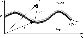
Fig. 4: Sketch of an interface $f(\mathbf{S})$, $\mathbf{S}\in\mathbb{R}^{2}$, and its normal coordinate system (NCS) consisting of a point $\mathbf{s}\in\mathbb{R}^{3}$ on $f$, its normal vector $\mathbf{n}$, and the normal distance $u$. Thus each point P has two representations, either as a vector $\mathbf{r}$ or as $\mathbf{s}+u\,\mathbf{n}$ within the NCS (see Eq. (47)). Additional assumptions are required to assure the unique equivalence of both (see main text). In the present picture the condition $|u|<R_{\mathit{min}}$ for all $u$ is violated because the normal distance of the point $P$ is larger than the radius of curvature of the right bump.

(For the following general remarks we omit the index $i$.)

To this end we consider the points $\mathbf{s}(\mathbf{S})=\big{(}\mathbf{S},f(\mathbf{S})\big{)}^{t}$ of the Monge parameterized surface $f(\mathbf{S})$, the normal vector $\mathbf{n}(\mathbf{S})$, and the map $\mathcal{T}:\mathbb{R}^{2}\times\mathbb{R}\rightarrow\mathbb{R}^{3}$ (see Fig. 4) so that

$$\mathcal{T}(\mathbf{S},u):=\mathbf{s}(\mathbf{S})+u\,\mathbf{n}(\mathbf{S})\,.$$ (47)

Thus, each spatial point $\mathbf{r}$ can be expressed in terms of a point on the surface $\mathbf{s}$ and its normal distance $u$ from the surface. However, finding $\mathbf{S}$ and $u$ for a given point $\mathbf{r}$, i.e., finding the solution of the equation $\mathbf{r}=\mathcal{T}\big{(}\mathbf{S}(\mathbf{r}),u(\mathbf{r})\big{)}$, is generally not a trivial task. However, in order to obtain a unique map $\mathcal{T}^{-1}$ we have to restrict the range of values of $u$ to $(-R_{\mathit{min}},R_{\mathit{min}})$ where $R_{\mathit{min}}>0$ denotes the absolute value of the minimal radius of curvature of the manifold $f(\mathbf{S})$. Therefore, the constraint $|u|<R_{\mathit{min}}$ guarantees, that the Jacobian $J_{f}$ of the transformation $\mathcal{T}$,

$$J_{f}(\mathbf{S},u) = \sqrt{g(\mathbf{S})}\,(1-2H(\mathbf{S})\,u+K(\mathbf{S})\,u^{2})\,,$$ (48)

does not vanish in the domain $\mathbb{R}^{2}\times(-R_{\mathit{min}},R_{\mathit{min}})$. Here, $H\equiv H(\mathbf{S})$ is the local mean curvature, $K\equiv K(\mathbf{S})$ is the local Gaussian curvature, and $g\equiv g(\mathbf{S})$ is the metric of the manifold $f(\mathbf{S})$ which in Monge representation takes the form $g(\mathbf{S})=1+\big{(}\nabla f(\mathbf{S})\big{)}^{2}$.

If $f(\mathbf{S})$ is an iso-density contour of $\rho_{f}(\mathbf{r})$, we may write for points $(\mathbf{S},u)\in\mathbb{R}^{2}\times(-R_{\mathit{min}},R_{\mathit{min}})$

$$\rho_{f}(\mathbf{r})=\tilde{\rho}_{f}(\mathbf{S},u)\,.$$ (49)

These expressions hold also for a flat surface which results in $\rho_{c}(z)=\tilde{\rho}_{c}(u)$ with $u=z-c$.

Similar to Eq. (3) we assume

$$\tilde{\rho}_{f_{i}}(\mathbf{S},u\rightarrow\pm R_{\mathit{min}})=\rho_{i}^{\pm}\,,\;i\in\{1,2\}\,.$$ (50)

Since Eq. (50) can be strictly valid only for macroscopicly large values of $u$, we assume that $R_{\mathit{min}}$ is sufficiently large so that Eq. (50) is fulfilled for all practical purposes. Now, we propose an expansion of the transformed density profile $\tilde{\rho}_{f_{i}}(\mathbf{S},u)$ into powers of the local curvatures $H_{i}\equiv H_{i}(\mathbf{S})$ and $K_{i}\equiv K_{i}(\mathbf{S})$, $i\in\{1,2\}$:

$$\tilde{\rho}_{f_{i}}(\mathbf{S},u) = \tilde{\rho}_{c_{i}}(u)+\delta\rho_{f_{i}}(\mathbf{S},u)$$ (51a)

$$\delta\rho_{f_{i}}(\mathbf{S},u) \approx \sum_{{{\alpha,\beta=0\atop\alpha+\beta\geq 1}}}(2H_{i})^{\alpha}\,K_{i}^{\beta}\,\rho_{H_{i}^{\alpha}K_{i}^{\beta}}(u)\;.$$ (51b)

For each term this implies a factorization of the dependencies on the lateral coordinates $\mathbf{S}$ and the normal distance $u$, reflecting the condition that the width of the interface $\xi$ should be small compared with the minimal radius of curvature, i.e., $\xi\ll R_{\mathit{min}}$. For the following calculations, it is not necessary to specify the functions $\rho_{\lambda}(u)$, $\lambda\in\{H,K,H^{2},HK,\ldots\}$, which depend only on the normal distance $u$ but are so far unknown explicitly. However, for quantitative predictions one has to use a model for $\rho_{\lambda}(u)$ (see, c.f., Subsec. III.1).

II.6 Mean Surface Approximation

Except for $\mathcal{H}_{h}$ (see Eq. (28)) the formulas derived above can be used to transform and to expand the various contributions of the Hamiltonian $\mathcal{H}$. For $\mathcal{H}_{h}$ both densities have to be evaluated at the same spatial point, but there is no rule telling which normal coordinate set should be used for the transformation, i.e., which local curvatures have to be used. In order to resolve this issue we construct a mean density distribution $\rho^{*}(\mathbf{r})$ with a corresponding iso-density contour $f^{*}(\mathbf{R})$, such that $h\big{(}\rho_{1}(\mathbf{r}),\rho_{2}(\mathbf{r})\big{)}=h^{*}(\rho^{*}(\mathbf{r}))$ where $h^{*}$ is a function to be determined, and use the normal coordinate system associated with $f^{*}(\mathbf{R})$ in order to transform $\mathcal{H}_{h}$ and to expand $h^{*}(\rho^{*}(\mathbf{r}))$. Since we know the relation between $f^{*}(\mathbf{R})$ and $f_{i}(\mathbf{R})$ explicitly, we are able to express the results in terms of $f_{i}$. We stress that this problem would equally arise for more sophisticated density functionals beyond the local density approximation used in Eq. (2).
We start our approach with an implicit definition of the points $\mathbf{r}^{*}$ fulfilling the constraint $\rho^{*}(\mathbf{r}^{*})=\mathit{const}$. First, we assume that the flat configuration can be written as (see Eqs. (4)-(6))

$$\tilde{\rho}_{c_{i}}(u)=-\,\frac{\triangle\rho_{i}}{2}\,\textrm{p}(u/\xi_{i})+\bar{\rho}_{i}$$ (52)

with an odd function $\textrm{p}(-\,x)=-\,\textrm{p}(x)$ so that $\textrm{p}(0)=0$. Second, we define, with a not yet specified prefactor $\triangle\rho^{*}$, the mean density

$$\rho^{*}(\mathbf{r}):=\triangle\rho^{*}\,\sum_{i=1}^{2}\,\frac{\tilde{\rho}_{f_{i}}\big{(}\mathbf{S}^{(i)}(\mathbf{r}),u_{i}(\mathbf{r})\big{)}}{\triangle\rho_{i}}\,\,.$$ (53)

The equation for the corresponding iso-density contour reads

$$\rho^{*}(\mathbf{r}^{*})=\overline{\rho^{*}}\,:=\,\triangle\rho^{*}\,\sum_{i=1}^{2}\frac{\bar{\rho}_{i}}{\triangle\rho_{i}}.$$ (54)

Using the expansion introduced in Eq. (51b), in lowest order this leads to

$$\sum_{i=1}^{2}\,\frac{\tilde{\rho}_{c_{i}}\big{(}u_{i}(\mathbf{r}^{*})\big{)}}{\triangle\rho_{i}}=0$$ (55)

and hence to the condition (using Eq. (52)) with $u_{i}^{*}\equiv u_{i}(\mathbf{r}^{*})$

$$\frac{u_{1}^{*}}{\xi_{1}}+\frac{u_{2}^{*}}{\xi_{2}}=0\,.$$ (56)

Thus, we postulate that the normal distances $u_{i}^{*}$ between $f_{i}$ and a point $\mathbf{r}^{*}$ on the iso-density manifold $f^{*}$, measured in units of the width $\xi_{i}$ of the corresponding interface, are equal (see Fig. 5); this is a construction scheme for $f^{*}$.

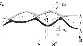
Fig. 5: Sketch of the construction scheme for the mean surface points $\mathbf{r}^{*}$. Since the points $\mathbf{r}^{*}$ represent an iso-density manifold $f^{*}$ of the mean density $\rho^{*}(\mathbf{r})$ they are determined in terms of the distances $u_{i}^{*}$ between the surfaces $f_{i}$ and $\mathbf{r}^{*}$ (see Eq. (56)) assuming that, normal to each surface $f_{i}$, the density profile has the form given by Eq. (52).

In general, the lateral coordinates $\mathbf{S}^{(1)}$ and $\mathbf{S}^{(2)}$ which belong to the same point $\mathbf{r}^{*}$ are different. We write $\mathbf{s}_{i}(\mathbf{r}^{*}):=\big{(}\mathbf{S}^{(i)}(\mathbf{r}^{*}),f_{i}(\mathbf{S}^{(i)}(\mathbf{r}^{*}))\big{)}\equiv\mathbf{s}_{i}^{*}$ for the corresponding point on the surface $f_{i}$ while $\mathbf{n}_{i}(\mathbf{r}^{*})\equiv\mathbf{n}_{i}^{*}$ denotes its normal vector there. Expressing $\mathbf{r}^{*}$ as

$$\mathbf{r}^{*}=a_{1}\,\mathbf{s}_{1}^{*}+a_{2}\,\mathbf{s}_{2}^{*}+\alpha_{1}\,\mathbf{n}_{1}^{*}+\alpha_{2}\,\mathbf{n}_{2}^{*}$$ (57)

with the coefficients $a_{i},\alpha_{i}\in\mathbb{R}$ to be determined. In combination with Eq. (56) one obtains

$$0=\sum_{{{i,j=1\atop i\neq j}}}^{2}\,\mathbf{s}_{i}^{*}\,\Big{(}\frac{a_{i}-1}{\xi_{i}}\,\mathbf{n}_{i}^{*}+\frac{a_{i}}{\xi_{j}}\,\mathbf{n}_{j}^{*}\Big{)}+\frac{\zeta_{i}}{\xi_{1}\xi_{2}}\,,$$ (58)

with $\alpha_{1}=\zeta_{1}/(\xi_{2}+\xi_{1}\,\mathbf{n}_{1}^{*}\mathbf{n}_{2}^{*})$, $\alpha_{2}=\zeta_{2}/(\xi_{1}+\xi_{2}\,\mathbf{n}_{1}^{*}\mathbf{n}_{2}^{*})$, and coefficients $\zeta_{i}\in\mathbb{R}$.
For the special case $\mathbf{s}_{1}^{*}=\mathbf{s}_{2}^{*}$ one has $\mathbf{r}^{*}=\mathbf{s}_{1}^{*}=\mathbf{s}_{2}^{*}$ which leads to the relation $a_{1}+a_{2}=1$ and $\alpha_{i}\sim|\mathbf{s}_{1}^{*}-\mathbf{s}_{2}^{*}|$. For symmetry reasons we set $a_{1}=a_{2}=\frac{1}{2}$ in order to treat the surfaces equally. We now consider the case $f_{2}(\mathbf{S})=-f_{1}(\mathbf{S})$ and $\xi_{1}=\xi_{2}$, which implies $\mathbf{S}^{(1)}=\mathbf{S}^{(2)}\equiv\mathbf{S}$ and $\mathbf{r}^{*}\,\mathbf{e}_{z}=0$, where $\mathbf{e}_{z}$ is the unit vector in the $z$ direction (see Fig. 5). With $\zeta_{1}=\frac{\xi_{1}}{2}\,(\mathbf{s}_{2}^{*}-\mathbf{s}_{1}^{*})\,\mathbf{n}_{2}^{*}$ and $\zeta_{2}=\frac{\xi_{2}}{2}\,(\mathbf{s}_{1}^{*}-\mathbf{s}_{2}^{*})\,\mathbf{n}_{1}^{*}$ this leads to

$$\mathbf{r}^{*}=\left(\begin{array}[]{c}\mathbf{S}+f_{1}(\mathbf{S})\nabla f_{1}(\mathbf{S})\\ 0\end{array}\right)\;\textrm{ and }\;u_{1}^{*}=-\sqrt{g_{1}(\mathbf{S})}\,f_{1}(\mathbf{S})\,,$$ (59)

so that Pythagoras’ theorem, $u_{1}^{*2}=(\mathbf{R}^{*}-\mathbf{S})^{2}+f_{1}^{2}(\mathbf{S})$, is fulfilled. (For different choices of $\zeta_{i}$ this is generally not the case.) This means that for $f_{2}(\mathbf{S})=-\,f_{1}(\mathbf{S})$ the manifold $f^{*}$ is the plane $z=0$. Using the same choice for $\zeta_{i}$ in the case $\xi_{1}\neq\xi_{2}$, Eq. (57) yields

$$\alpha_{1}=\frac{\xi_{1}\,\big{[}\mathbf{s}_{2}^{*}-\mathbf{s}_{1}^{*}\big{]}\,\mathbf{n}_{2}^{*}}{2\,(\xi_{2}+\xi_{1}\,\mathbf{n}_{1}^{*}\mathbf{n}_{2}^{*})}\quad,\quad\alpha_{2}=\frac{\xi_{2}\,\big{[}\mathbf{s}_{1}^{*}-\mathbf{s}_{2}^{*}\big{]}\,\mathbf{n}_{1}^{*}}{2\,(\xi_{1}+\xi_{2}\,\mathbf{n}_{1}^{*}\mathbf{n}_{2}^{*})}$$ (60)

so that the distances $u_{i}^{*}$ fulfill

$$\frac{u_{1}^{*}}{\xi_{1}}=\frac{\alpha_{1}}{\xi_{1}}-\frac{\alpha_{2}}{\xi_{2}}=-\frac{u_{2}^{*}}{\xi_{2}}\,.$$ (61)

Nonetheless, Eq. (57) still is an implicit expression for $\mathbf{r}^{*}$ which represents approximately points on the iso-density manifold $f^{*}$ of $\rho^{*}(\mathbf{r})$.
Since $f_{1}$ and $f_{2}$ are assumed to not exhibit strong variations on short scales, this translates to $f^{*}$ so that $\mathbf{r}^{*}$ allows for a Monge parametrisation $\mathbf{r}^{*}=(\mathbf{R}^{*},f^{*}(\mathbf{R}^{*}))$, too. Hence in Eq. (57) we can use a Taylor expansion $f_{i}(\mathbf{S}^{(i)})\approx f_{i}(\mathbf{R}^{*})+\nabla f_{i}(\mathbf{R}^{*})\,(\mathbf{S}^{(i)}-\mathbf{R}^{*})$ which leads in lowest order to (Eq. (60))

$$\frac{f^{*}(\mathbf{R}^{*})}{\xi^{*}}=\frac{1}{2}\,\sum_{i=1}^{2}\frac{f_{i}(\mathbf{R}^{*})}{\xi_{i}}\quad,\;\xi^{*}:=\frac{2\xi_{1}\xi_{2}}{\xi_{1}+\xi_{2}}\,.$$ (62)

A more sophisticated calculation, which takes additional curvature corrections in Eq. (55) into account, i.e., using the next higher order terms in Eq. (51b), shows that corrections to Eq. (62) are of the order $\mathcal{O}(f_{i}^{n}f_{j}^{m},n+m\geq 3)$. Since in Sec. III we shall consider the Hamiltonian $\mathcal{H}$ within a Gaussian approximation the expression in Eq. (62) is sufficient. Furthermore, from Eq. (62) it follows that the surface with a smaller interfacial width $\xi$ contributes stronger to $f^{*}$.

To summarize Sec. II, from the density functional $\Omega$ in Eq. (1) for a binary liquid mixture, in Eq. (27) we have introduced an effective interface Hamiltonian $\mathcal{H}$ by specifying an iso-density contour $f_{i}$ for each density profile $\rho_{i}$ as its corresponding interface, which compose the interface of the mixture as a whole, and by comparing them with the corresponding flat reference configurations. In order to express $\mathcal{H}$ in terms of the manifolds $f_{i}$ we used an expansion of the densities in powers of curvatures of $f_{i}$ (see Eq. (51b)). Since the hard sphere contribution $\mathcal{H}_{h}$ cannot be treated within this approximation, we have constructed an effective mean surface $f^{*}$ (see Eq. (62)), which itself is an iso-density contour of a composed density $\rho^{*}$, so that the curvature expansion can be performed regarding $f^{*}$ and $\rho^{*}$. The results of the curvature expansion of $\mathcal{H}$ up to second order are presented in the next chapter. Since all expressions would become rather clumsy without using short notations, we shall introduce additional abbreviations in order to obtain a clear presentation of the structure of the formulas.

III Gaussian Approximation

In the previous chapter we have illustrated the basic ideas and have derived the general expressions which arise upon introducing the effective interface Hamiltonian. In this section we carry out the curvature expansion in Eq. (51b) up to second order. Higher order terms are given explicitly in Appendix A. Since in the following the profiles $\rho_{c_{i}}(z)$ do no longer occur we drop the tilde in $\tilde{\rho}_{c}(u)$ and write $\rho_{c}(u)$ instead (see Eqs. (49)-(51b)).
First, we provide some numerical aspects which enter into the graphical presentation given below. Within the Gaussian approximation $\mathcal{H}$ is determined by the profiles $\rho_{c}$ and $\rho_{H}$ and the interaction potentials $w_{ij}$ given in Eq. (18). For $\rho_{c_{i}}$ we use Eq. (52) with an intrinsic profile $\textrm{p}(x)=\tanh(x/2)$ and, guided by Ref. Mecke and Dietrich (1999), for $\rho_{H_{i}}$ we choose

$$\frac{\rho_{H_{i}}(u)}{\triangle\rho_{i}}=C_{N}\,r_{o}^{(i)}\,\frac{x\,\textrm{p}(2\,x)}{2\pi\,\cosh(x)}\;,\;x\equiv\frac{u}{2\,\xi_{i}}\,,$$ (63)

with a dimensionless positive number $C_{N}$. Comparing this expression with the analogous one, $\rho_{H}$, for the one-component fluid introduced in Eq. (3.27) in Ref. Mecke and Dietrich (1999) with a prefactor $C_{H}$, one obtains $C_{N}\,r_{o}^{(i)}=C_{H}\,\xi_{i}$. Thus, different from Ref. Mecke and Dietrich (1999) here we assume, that the prefactor $C_{N}\,r_{o}^{(i)}$ does not vary with temperature. This choice here translates into that in Ref. Mecke and Dietrich (1999) if there one takes $C_{H}\sim\xi^{-1}\rightarrow 0$ for $T\rightarrow T_{c}$. Therefore, $\rho_{H_{i}}/\triangle\rho_{i}$ remains bounded for all temperatures, so that the curvature influence characterized by $\rho_{H_{i}}$ vanishes $\sim\triangle\rho_{i}$ for $T\rightarrow T_{c}$. In Ref. Mecke and Dietrich (1999), $\rho_{H}/\triangle\rho_{i}$ diverges $\sim\xi$ for $T\rightarrow T_{c}$, so that in that temperature range the influence of the curvature may even dominate. Therefore we prefer the choice given in Eq. (63) A more detailed discussion of a possible temperature dependence of $C_{H}$ can be found in Ref. Hiester (2005). For reasons of simplicity, in the following we consider only the case $C_{N}=1.0$. We emphasize that the structural properties found in Ref. Mecke and Dietrich (1999) do not change if $C_{H}\sim\xi^{-1}$ instead of being constant.
While the ratio $r_{o}^{(1)}/r_{o}^{(2)}$ of the radii of the particles is a free parameter, the temperature dependent correlation lengths $\xi_{i}$ are determined by the bulk correlation functions. In terms of the total bulk density $\rho$ the concentrations $\rho_{i}=X_{i}\,\rho$ fulfill $X_{1}+X_{2}=1$. From the Ornstein-Zernike theory for mixtures one has

$$\xi_{i}^{2} = -\frac{\rho^{2}}{2}\,\chi_{T}\,\sum_{i=1}^{2}\int_{V}\,d^{3}r\,r^{2}w_{ij}(r)$$ (64)

with the isothermal compressibility $\chi_{T}=\frac{1}{\rho}\big{(}\frac{\partial\rho}{\partial p}\big{)}_{T,V}$, which can be expressed as

$$\chi_{T}=\frac{1}{\rho^{2}}\,\bigg{[}\,\frac{d^{2}h(\rho X_{1},\rho X_{2})}{d\rho^{2}}+\sum_{i,j=1}^{2}\int_{V}\,d^{3}r\,X_{i}X_{j}\,w_{ij}(r)\,\bigg{]}^{-1}\,.$$ (65)

For the two coexisting phases liquid and vapor the two corresponding total densities $\rho^{\pm}$ lead to different values $\chi_{T}^{\pm}$ and thus $\xi_{i}^{\pm}\equiv\xi_{i}(\rho^{\pm})$. In the subsequent numerical calculations we use $\xi_{i}=(\xi_{i}^{+}+\xi_{i}^{-})/2$ (see also the caption of Fig. 3).

III.1 General Expression

As stated at the beginning of this section we consider only contributions to $\mathcal{H}$ up to 2nd order in the deviations $f_{i}^{c}$ of the local interface height from the flat configuration. With $\hat{\mathbf{f}}(\mathbf{q})$ as the Fourier transform of the vector $\mathbf{f}(\mathbf{R})$ (see Eqs. (26) and (40)), one has

$$\mathcal{H}^{G}[\hat{\mathbf{f}}(\mathbf{q})]=\frac{1}{4\pi}\int_{A}\!d^{2}q\;\;\hat{\mathbf{f}}^{{\dagger}}(\mathbf{q})\;\mathbb{E}(q)\;\hat{\mathbf{f}}(\mathbf{q})\,\$$ (66)

with

$$\mathbb{E}(q):=\mathbb{G}(q)+\mathbb{W}(q)+q^{4}\,\mathbb{K}\,.$$ (67)

Here, the matrix $\mathbb{G}(q)$ represents the contributions stemming from gravity (see Eq. (152)), the matrix $\mathbb{W}(q)$ captures the influence of the attractive interaction potentials (see Eq. (154)), and the constant matrix $\mathbb{K}$ involves hard sphere contributions (see Eq. (139)). The explicit expressions for $\mathbb{G}$, $\mathbb{W}$, and $\mathbb{K}$ are derived in Appendix B, where the equilibrium condition for the planar densities $\rho_{c_{i}}(u)$ (Eq. (8)) is frequently used to obtain the final form of $\mathbb{E}(q)$.
In order to be able to present our results in a compact form we introduce the following abbreviations. For an integer $n\geq 0$ and arbitrary expressions $\mathcal{A}_{i}\equiv\mathcal{A}_{i}(u,\ldots)$ we define the moments (similar as in Ref. Mecke and Dietrich (1999))

$$\delta_{n}[\mathcal{A}_{i}] = \frac{1}{\triangle\rho_{i}}\,\int_{-R_{\mathit{min}}}^{R_{\mathit{min}}}\!\!du\,u^{n}\,\mathcal{A}_{i}(u,\ldots)\,.$$ (68)

With this notation, the matrix elements of $\mathbb{G}(q)$ can be expressed as ($\delta_{\alpha\beta}$ is the Kronecker symbol)

$$\mathbb{G}_{11} = G\,m_{1}\triangle\rho_{1}\,\Big{[}1-2q^{2}\,\Big{(}\delta_{o}[\rho_{H_{1}}]$$ (69)

$$\!\!\!\!\!\!\!+\,\sum_{k=1}^{2}(\delta_{k1}-d_{2}^{2})\,\big{(}\delta_{2}[\partial_{u}\rho_{c_{k}}]+q^{2}\,\delta_{2}[\rho_{H_{k}}]\big{)}\Big{)}\Big{]}$$

with $d_{i}\,=\,\xi_{i}/(\xi_{1}+\xi_{2})$ and similarly for $\mathbb{G}_{22}$ by interchanging the indices $1\leftrightarrow 2$ and ($\mathbb{G}_{12}=\mathbb{G}_{21}$)

$$\mathbb{G}_{12}=2q^{2}\,d_{1}d_{2}\sum_{i=1}^{2}G\,m_{i}\triangle\rho_{i}\,\Big{(}\delta_{2}[\partial_{u}\rho_{c_{i}}]+q^{2}\,\delta_{2}[\rho_{H_{i}}]\Big{)}\,.$$ (70)

The first part of Eq. (69) up to $\delta_{o}[\rho_{H_{1}}]$ is identical with the corresponding expression in Ref. Mecke and Dietrich (1999), and is recovered by setting $\triangle\rho_{2}=0$ and $\xi_{2}\rightarrow\infty$ (which results in $d_{1}=0$ and $d_{2}=1$), which consequently implies $f^{*}\equiv f_{1}$ from Eq. (62). All further parts in Eq. (69) arise due to the presence of a second interface. This is somewhat surprising, because the gravity terms of the density functional $\Omega$ are diagonal in the densities and thus, one expects $\mathbb{G}(q)$ to be diagonal w.r.t. the surfaces, too. Actually, the additional terms in Eq. (69) and $\mathbb{G}_{12}(q)\neq 0$ emerge by applying the equilibrium condition in Eq. (8) in order to get rid of certain hard-sphere contributions from $\mathcal{H}_{h}$ (Eq. (28)). All remaining hard-sphere contributions are captured by the matrix $\mathbb{K}=\big{(}\mathbb{K}_{ij}\big{)}_{i,j\in\{1,2\}}$ with

$$\mathbb{K}_{ij}=\int_{-R_{\mathit{min}}}^{+R_{\mathit{min}}}\!du\;\partial_{\rho_{i}\rho_{j}}^{2}h\big{(}\rho_{c_{1}}(u),\rho_{c_{2}}(u)\big{)}\,\,\rho_{H_{i}}(u)\rho_{H_{j}}(u)\,.$$ (71)

$\mathbb{K}$ has the form expected as the generalization to two components of the analogous term $\kappa$ in Ref. Mecke and Dietrich (1999).
The matrix $\mathbb{W}(q)$ depends on the pair potentials. Hence, for $k\in\{0,1,2\}$ it is convenient to use the short notation $\hat{w}_{ij}^{(k)}[q,\delta c_{ij}]:=\hat{w}_{ij}^{(k)}(q,u^{\prime}-u^{\prime\prime}+\delta c_{ij})$ for the Fourier transformed interaction potential (see Eq. (42)) or the integrals of it (see Eqs. (19) and (20)), respectively. Moreover, similar to Eq. (68) for an expression $\mathcal{A}_{ij}\equiv\mathcal{A}_{ij}(u^{\prime},u^{\prime\prime},\ldots)$ we define the moments

$$\hat{\omega}^{(k)}(q,\mathcal{A}_{ij}):=\iint_{-R_{\mathit{min}}}^{R_{\mathit{min}}}\!\!du^{\prime}du^{\prime\prime}\,\,\hat{w}_{ij}^{(k)}[q,\delta c_{ij}]\,\mathcal{A}_{ij}(u^{\prime},u^{\prime\prime},\ldots)$$ (72)

and the differences

$$\delta\hat{\omega}^{(k)}(q,\cdots):=\hat{\omega}^{(k)}(q,\cdots)-\hat{\omega}^{(k)}(0,\cdots)\,,$$ (73)

but on the lhs we suppress the indices $c$ and the square brackets around $\mathcal{A}_{ij}$ indicating the functional dependence on $\mathcal{A}_{ij}$. In addition we use $\hat{\omega}^{(0)}(\ldots)\equiv\hat{\omega}(\ldots)$ due to $w_{ij}^{(0)}(\ldots)\equiv w_{ij}(\ldots)$ and similarly $\delta\hat{\omega}^{(0)}(\ldots)\equiv\delta\hat{\omega}(\ldots)$. Then, the entries of the matrix $\mathbb{W}(q)$ can be written as ($\partial_{{}^{\prime}}\equiv\partial_{u^{\prime}}$, $\partial_{{}^{\prime\prime}}\equiv\partial_{u^{\prime\prime}}$)

$$\mathbb{W}_{11}(q)=-\,\hat{\omega}\big{(}0,\partial_{{}^{\prime}}\rho_{c_{1}}\partial_{{}^{\prime\prime}}\rho_{c_{2}}\big{)}+\delta\hat{\omega}\big{(}q,\partial_{{}^{\prime}}\rho_{c_{1}}\partial_{{}^{\prime\prime}}\rho_{c_{1}}\big{)}\\ +\,2\,q^{2}\,\Big{[}\delta\hat{\omega}\big{(}q,\rho_{H_{1}}(u^{\prime})\partial_{{}^{\prime\prime}}\rho_{c_{1}}\big{)}-\hat{\omega}\big{(}0,\rho_{H_{1}}(u^{\prime})\partial_{{}^{\prime\prime}}\rho_{c_{2}}\big{)}\\ +\,\sum_{i,j=1}^{2}(d_{2}^{2}-\delta_{i1})\,\hat{\omega}^{(1)}\big{(}0,u^{\prime}\partial_{{}^{\prime}}\rho_{c_{i}}\partial_{{}^{\prime\prime}}\rho_{c_{j}}\big{)}\Big{]}\\ +\,q^{4}\,\Big{[}\,2\sum_{i,j=1}^{2}(d_{2}^{2}-\delta_{i1})\,\hat{\omega}^{(1)}\big{(}0,u^{\prime}\rho_{H_{i}}(u^{\prime})\partial_{{}^{\prime\prime}}\rho_{c_{j}}\big{)}\\ +\hat{\omega}\big{(}q,\rho_{H_{1}}(u^{\prime})\rho_{H_{1}}(u^{\prime\prime})\big{)}+2\sum_{j=1}^{2}\hat{\omega}^{(2)}(0,\rho_{H_{1}}(u^{\prime})\partial_{{}^{\prime\prime}}\rho_{c_{j}})\Big{]}$$ (74)

and ($\mathbb{W}_{12}=\mathbb{W}_{21}$)

$$\mathbb{W}_{12}(q) = \hat{\omega}\big{(}q,\partial_{{}^{\prime}}\rho_{c_{1}}\partial_{{}^{\prime\prime}}\rho_{c_{2}}\big{)}$$

$$+\,q^{2}\sum_{i,j=1}^{2}\bigg{\{}\,(1-\delta_{ij})\,\hat{\omega}\big{(}q,\rho_{H_{i}}(u^{\prime})\partial_{{}^{\prime\prime}}\rho_{c_{j}}\big{)}$$

$$\qquad\qquad\;+\,2\,d_{1}d_{2}\,\hat{\omega}^{(1)}\big{(}0,u^{\prime}\partial_{{}^{\prime}}\rho_{c_{i}}\partial_{{}^{\prime\prime}}\rho_{c_{j}}\big{)}$$

$$\qquad+\,q^{2}\,\Big{[}2\,d_{1}d_{2}\,\hat{\omega}^{(1)}\big{(}0,u^{\prime}\rho_{H_{i}}(u^{\prime})\partial_{{}^{\prime\prime}}\rho_{c_{j}}\big{)}$$

$$\qquad+\,\frac{(1-\delta_{ij})}{2}\,\hat{\omega}\big{(}q,\rho_{H_{i}}(u^{\prime})\rho_{H_{j}}(u^{\prime\prime})\big{)}\Big{]}\bigg{\}}\,.$$

$\mathbb{W}_{22}(q)$ is obtained by interchanging the labels $1\leftrightarrow 2$ in $\mathbb{W}_{11}(q)$. Again, the result for a single interface is included as a limiting case by setting $\triangle\rho_{2}=0$, $d_{1}=0$, and $d_{2}=1$ (or equivalently $\xi_{2}\rightarrow\infty$) in Eqs. (74) and (III.1), which gives $\mathbb{W}_{12}=\mathbb{W}_{22}=0$ and $f^{*}\equiv f_{1}$ from Eq. (62). All additional terms are generated by applying the equilibrium condition in Eq. (8). Although these expressions are useful to determine numerically the matrix elements $\mathbb{E}_{ij}(q)$, the formal structure of $\mathbb{E}(q)$ might be more transparent in the presentation given in Eq. (161).
In order to obtain further insight into the nature of $\mathcal{H}$ it is useful to transform $\mathbb{E}$ into a diagonal matrix. To this end, we define

$$\lambda_{i}(q) := \mathbb{E}_{ii}(q)+\mathbb{E}_{12}(q)\,,$$ (76)

$$\Lambda^{+}(q) := \lambda_{1}(q)+\lambda_{2}(q)\,,$$ (77)

and

$$\Lambda^{-}(q) := \frac{\det\mathbb{E}(q)}{\Lambda^{+}(q)}\,.$$ (78)

Furthermore, we define a “mean” surface $f^{+}$, and a “relative” surface $f^{-}$ via

$$\hat{f}^{+}(\mathbf{q}) := \sum_{i=1}^{2}\frac{\lambda_{i}(q)}{\lambda_{1}(q)+\lambda_{2}(q)}\,\,\hat{f}_{i}^{c}(\mathbf{q})$$ (79)

and

$$\hat{f}^{-}(\mathbf{q}) := \hat{f}_{2}^{c}(\mathbf{q})-\hat{f}_{1}^{c}(\mathbf{q})\,,$$ (80)

the fluctuations of which are decoupled within the Gaussian approximation, in contrast to $f_{1}^{c}$ and $f_{2}^{c}$. This leads to

$$\mathcal{H}^{G}[\hat{\mathbf{f}}(\mathbf{q})]=\frac{1}{4\pi}\int_{A}\!d^{2}q\,\sum_{\alpha\in\{+,-\}}\,\Lambda^{\alpha}(q)\,|\hat{f}^{\alpha}(\mathbf{q})|^{2}\,.$$ (81)

This resembles some similarity to the decomposition of the two-body problem in classical mechanics. It is important to note that $\Lambda^{\pm}(q)$ are not the eigenvalues of $\mathbb{E}(q)$ since the coordinate transformation used and defined by Eqs. (79) and (80) is not orthonormal. Moreover, this transformation makes sense only for $\lambda_{j}\neq 0$. Therefore, the limiting case of a single component is better discussed in terms of Eqs. (66) and (67) as mentioned above.

III.2 Energy Density $\Lambda^{+}(q)$

Fig. 6: Normalized wave-vector dependent surface energy $\gamma^{+}(q)/\gamma^{+}(0)$ as defined by Eq. (83) for different temperatures $T=0.7\ldots 0.99\,T_{c}$, where $T_{c}$ is the bulk critical point of the binary liquid mixture in coexistence with its vapor, computed from the grand canonical density functional in Eq. (1). The size ratio is $r_{o}^{(2)}/r_{o}^{(1)}=1.001$ with $r_{o}^{(12)}=r_{o}^{(1)}+r_{o}^{(2)}$ and $w_{o}^{(22)}/w_{o}^{(11)}=1.05$, $w_{o}^{(12)}/w_{o}^{(11)}=0.5$ for the depths of the interaction potentials (see Eq. (18)). $\delta c_{12}$ is set to $0$, but $\gamma^{+}(q)/\gamma^{+}(0)$ depends only weakly on $\delta c_{12}$ for $|\delta c_{12}|\leq 5\,r_{o}^{(12)}$. Here, $C_{N}=1$ (see Eq. (63)); another choice $C_{N}>1$ modifies mainly the bending constants $\mathbb{K}_{ij}$ (see Eq. (139)) and thus the curves increase stronger for larger values of $q$ beyond the minimum which is also shifted to larger wavelengths $1/q$. The opposite behavior is observed for $C_{N}<1$. For low temperatures the minimum is rather deep and occurs at large $q$ values. Upon raising the temperature the minimum becomes more and more shallow and moves to smaller values of $q$, too. This is the same qualitative behavior as observed for the one component case Mecke and Dietrich (1999).

The quantity $\Lambda^{+}(q)$ can be written as

$$\Lambda^{+}(q)=G\,\mathcal{G}^{+}(q)+q^{2}\gamma^{+}(q)$$ (82)

where $\mathcal{G}^{+}(q)=\mathcal{G}_{1}(q)+\mathcal{G}_{2}$ with $\mathcal{G}_{i}=m_{j}\triangle\rho_{j}\,\big{(}1-2q^{2}\,\delta_{o}[\rho_{H_{j}}]\big{)}$ (Eq. (122)), and $\gamma^{+}(q)$ takes the form

$$\gamma^{+}(q):=\sum_{i,j=1}^{2}\,\gamma_{ij}(q)$$ (83)

with

$$\gamma_{ij}(q) = \frac{\delta\hat{\omega}\big{(}q,\partial_{{}^{\prime}}\rho_{c_{i}}\partial_{{}^{\prime\prime}}\rho_{c_{j}}\big{)}}{q^{2}}+\,2\,\delta\hat{\omega}\big{(}q,\rho_{H_{i}}\partial_{{}^{\prime\prime}}\rho_{c_{j}}\big{)}$$

$$+\,q^{2}\,\Big{[}\,\hat{\omega}\big{(}q,\rho_{H_{i}}\rho_{H_{j}}\big{)}+\mathbb{K}_{ij}+\,2\hat{\omega}^{(2)}(0,\rho_{H_{i}}\partial_{{}^{\prime\prime}}\rho_{c_{j}})\Big{]}$$. (84)

This formula is the generalization of the corresponding result derived for a one-component fluid Mecke and Dietrich (1999), except that the term $\hat{\omega}^{(2)}(0,\rho_{H_{i}}\partial_{{}^{\prime\prime}}\rho_{c_{j}})$ shows up additionally. $\gamma^{+}(q)$ is plays the role of a wavevector dependent surface tension for $f^{+}$, which then behaves similarly as for a single interface. Since according to Eq. (79) $\hat{f}^{+}(q)$ is a linear combination of the surfaces, $\hat{f}_{j}^{c}$ can be considered as the prime or mean surface of the binary fluid. The functional form of $\gamma^{+}(q)$ is shown in Fig. 6 for various temperatures.

III.3 Energy Density $\Lambda^{-}(q)$

Fig. 7: Normalized wavevector dependent free energy density $\Lambda^{-}_{o}(q)/\Lambda^{-}_{o}(0)$ as given by Eq. (85) for various temperatures $T=0.7\ldots 0.99\,T_{c}$. The choices for the interaction potentials are $r_{o}^{(2)}/r_{o}^{(1)}=1.001$ for the radii and $w_{o}^{(22)}/w_{o}^{(11)}=1.05$, $w_{o}^{(12)}/w_{o}^{(11)}=0.5$ for the interaction strengths (see Eq. (18)). $\delta c_{12}$ is taken to be $0$. Distinct from the normalized surface tension $\gamma^{+}(q)$ shown in Fig. 6, $\Lambda^{-}_{o}(q)$ shows a monotonic increase at low temperatures, but forms a minimum at a nonzero value of $q$ if the temperature is increased. As for $\gamma^{+}(q)$, this minimum is shifted to larger wavelengths upon further increasing the temperature. It is important to note, that $\Lambda^{-}_{o}(q)$ reflects the free energy density of different surface configurations of $f^{-}$ but it is not a surface tension because no Goldstone modes, i.e., translational shifts without cost in free energy, exist for $f^{-}$ as they do for $f^{+}$. Moreover, for $q>0$ one expects $0<\Lambda^{-}_{o}(q)\sim\det\mathbb{E}(q)$ for stability reasons.

$\Lambda^{-}(q)$ is determined by Eq. (78). It exhibits a more complex structure than $\Lambda^{+}(q)$. The explicit expression for $\det\mathbb{E}(q)$ is given by Appendix C. The intrinsic behavior of the surfaces is given by the pair potentials of the particles alone, independent of the external field. Thus in the absence of gravity, i.e., for $G=0$, one obtains the undisturbed energy density $\Lambda^{-}_{o}(q)=\Lambda^{-}(q,G=0)$ of the different surface configurations $f^{-}$. Similar to $\Lambda^{+}(q)$ it can be decomposed into a wave-vector dependent surface tension $\gamma^{-}(q)$ and an additional contribution that does not vanish for $q\rightarrow 0$ and which depends parametrically only on the interaction potential $w_{12}$ between the two species and the planar density profiles $\partial_{u}\rho_{c_{i}}$ (see Eq. (72) for $\hat{\omega}$):

$$\Lambda^{-}_{o}(q)=-\,\hat{\omega}\big{(}0,\partial_{{}^{\prime}}\rho_{c_{1}}\partial_{{}^{\prime\prime}}\rho_{c_{2}}\big{)}+q^{2}\,\gamma^{-}(q)\,.$$ (85)

$\Lambda^{-}_{o}(q)$ describes the free energy required to deform the relative surface into a corrugated one with a wave-vector $q$ in the presence of the microscopic interactions of the particles. For $q=0$ one has $\Lambda^{-}_{o}(0)>0$, which corresponds to the free energy needed to separate the flat equilibrium surfaces $c_{1}$ and $c_{2}$ from each other. This is in accordance with the facts, that $\Lambda^{-}_{o}(0)$ depends on $w_{12}$ and significantly weakens for larger $\delta c_{12}$ for which $f_{2}^{c}$ and $f_{1}^{c}$ decouple. In addition, at low temperatures $\Lambda^{-}_{o}(q)$ varies sensitively upon changes of $\delta c_{12}$, but it hardly changes its character at higher temperatures. This can be explained heuristically by noting that for $T\lesssim T_{c}$ the dominant length scale is set by the diverging bulk correlation length $\xi$ so that the difference $\delta c_{12}$ becomes irrelevant for the statistical weights.

$\Lambda^{-}_{o}(q)$ differs from $\gamma^{+}(q)$ qualitatively (see Fig. 7 and note that $\Lambda^{+}(q,G=0)/\Lambda^{+}(q\rightarrow 0,G=0)=\gamma^{+}(q)/\gamma^{+}(0)$ according to Eq. (83)): for temperatures close to the triple point, it shows a monotonic increase implying that surface configurations $f^{-}$ with nonzero wavelengths are energetically suppressed. But for higher temperatures a minimum at $q\neq 0$ evolves. This minimum is also shifted towards longer wavelengths for further increased temperatures but does not change its depth. Thus, together with the behavior of $\gamma^{+}(q)$, this means that for low temperatures the mean surface $f^{+}$ is more easily excited thermally than the relative surface $f^{-}$. But for higher temperatures, the thermal fluctuations have a stronger influence on $f^{-}$ while $f^{+}$ becomes more rigid. This behavior is quantitatively controlled by the curvature corrections characterized by $\rho_{H}$ (see Eq. (63)) and thus $C_{N}$. The influence of $C_{N}$ on $\Lambda^{-}_{o}(q)$ becomes mainly visible through a shift of the depth of the minimum, which increases strongly for larger values of $C_{N}$. Thus, $\Lambda^{-}_{o}(q)$ may even become negative for certain values of $C_{N}$. In the absence of gravity, i.e. for $G=0$, one has $\Lambda^{-}_{o}(q)\sim\det\mathbb{E}(q)$ and thus $\Lambda^{-}_{o}(q)<0$ means that the system becomes unstable. By switching off all interactions between the two species, i.e., for $w_{12}=0$ the simple expression

$$\Lambda^{-}_{o}(q)=q^{2}\,\frac{\gamma_{11}(q)\,\gamma_{22}(q)}{\gamma_{11}(q)+\gamma_{22}(q)}\quad,\quad\,w_{12}\equiv 0\,,$$ (86)

emerges, so that from Eqs. (82) and (85) the relation $\gamma^{-}(q)\,\gamma^{+}(q)=\gamma_{11}(q)\,\gamma_{22}(q)$ follows.

In the general case of nonzero $w_{12}$ the expressions for $\gamma_{ij}$ in Eq. (84), for $\gamma^{\wedge}_{12}$ in Eq. (131), and for $\gamma^{\vee}_{ij}$ in Eq. (134) together with

$$\Gamma_{1}(q) := \gamma_{11}(q)+\frac{\gamma^{\wedge}_{12}(q)+\gamma^{\vee}_{12}(q)}{q^{2}}$$ (87)

and

$$\Gamma_{2}(q) := \gamma_{22}(q)+\frac{\gamma^{\wedge}_{12}(q)+\gamma^{\vee}_{21}(q)}{q^{2}}$$ (88)

lead to the following expression for $\gamma^{-}(q)$ as defined in Eq. (85) (see Eq. (145) for $d_{i}$ and Eq. (151) for $\mathscr{W}_{ij}$)

$$\gamma^{-}(q) = \frac{\hat{\omega}\big{(}0,\partial_{{}^{\prime}}\rho_{c_{1}}\partial_{{}^{\prime\prime}}\rho_{c_{2}}\big{)}-\gamma^{\wedge}_{12}(q)}{q^{2}}+\frac{\Gamma_{1}(q)\Gamma_{2}(q)}{\gamma^{+}(q)}$$ (89)

$$-\,2\,d_{1}d_{2}\displaystyle{\sum_{i,j=1}^{2}}\mathscr{W}_{ij}(q)+\gamma_{\mathsf{asym}}^{-}(q)\,.$$

The last term $\gamma_{\mathsf{asym}}^{-}(q)$ (see Eq. (156) in Appendix C) turns out to be the smallest contribution and it is determined by the contrast between the two species. The terms in Eq. (89) are listed according to their quantitative importance. The behavior of $\gamma^{-}(q)$ is determined mainly by the first and the second term, while the third one is about one order of magnitude smaller than the previous ones, and the last one may be smaller by even two orders of magnitude. $\gamma^{-}(q)$ captures the wavelength dependence of $\Lambda^{-}_{o}(q)$ (see Eq. (85)). A comparison between $\gamma^{+}$ and $\gamma^{-}$ (see Fig. 8) shows, that $\gamma^{-}(q)/\gamma^{-}(0)$ also exhibits a minimum at a nonzero wavevector but its depth increases with increasing temperature. Hence, for large values of $C_{N}$, $\gamma^{-}(q)$ and even $\gamma^{-}(0)$, which depends on $C_{N}$, too (see Eq. (89)), may become negative which probably indicates a breakdown of the Gaussian approximation or even of the concept of a relative surface. Nevertheless, for increasing temperatures its minimum is shifted to smaller values of $q$, analogous to the behavior of $\gamma^{+}(q)/\gamma^{+}(0)$. Quantitatively, one finds $\gamma^{-}(q)/\gamma^{+}(q)\lesssim 0.1$ for all values of $q$ and temperatures $T\lesssim 0.9\,T_{c}$ ($\gamma^{-}(q)/\gamma^{+}(q)\lesssim 0.2$ for $T\lesssim 0.99\,T_{c}$), so that $\gamma^{-}(q)$ is about one order of magnitude smaller than $\gamma^{+}(q)$. Therefore, one may regard the mean surface $f^{+}$ to be more rigid than the relative surface $f^{-}$.
Recently diffuse X-ray scattering data from the liquid-vapor interfaces of Bi:Ga, Tl:Ga, and Pb:Ga binary liquid alloys rich in Ga have been reported Li et al. (2006). In order to interpret these data the authors put forward an expression similar to Eq. (83) (see Eqs. (8)-(11) in Ref. Li et al. (2006)), in which, however, different than in Eqs. (83) and (84) only the curvature correction profile $\rho_{H_{2}}(u)$ of the segregated component was used without taking into account the profile $\rho_{H_{1}}(u)$ of the majority component, i.e., $\rho_{H_{1}}(u)\equiv 0$. Thus it appears to be highly rewarding to reanalyze these experimental data in a future contribution on the basis of the present full statistical description. This description might also provide an understanding of recent synchrotron X-ray reflectivity data on the interfacial width, broadened by capillary waves, of the liquid-liquid interface of nitrobenzene and water Luo et al. (2006); Benjamin (1997). However, this would require to extent the present analysis to binary dipolar fluids Szalai and Dietrich (2005). Furthermore, a recent analysis of the fluctuation spectrum of lipid bilayer shows similarities to our description in terms of two interfaces Brannigan and Brown (2006). These authors also define a mean and a relative surface (see Eqs. (5) and (6) in Ref. Brannigan and Brown (2006)) in order to take into account conformations of the bilayer via fluctuation modes of the bilayer thickness and of the bending modes of the mean surface of the bilayer. Their choice of boundary conditions leads to a decoupling of these modes in real space and an effective free energy for the bilayer deformations on both short and long wavelengths is derived (Eq. (21) in Ref. Brannigan and Brown (2006)). The main difference to our approach consists in their specific choice of boundary conditions for lipid bilayers, which cannot be applied to fluid interfaces. Accordingly, within the Gaussian approximation, in our approach a mode decoupling between $f^{+}$ and $f^{-}$ is achieved only in Fourier space, where $\hat{f}^{+}$ is defined as a wavelength-dependent weighted sum of the Fourier modes of the surfaces $\hat{f}_{1}$ and $\hat{f}_{2}$ (see Eqs. (79)-(81)). Consequently, $f^{+}$ consists of a sum of corresponding convolutions, which, in general, cannot be written as a sum of $f_{1}$ and $f_{2}$ with constant weights as it is done in Ref. Brannigan and Brown (2006). Nevertheless, in Subsec. II.6 we have also introduced a concept similar to the one used in Ref. Brannigan and Brown (2006). In Subsec. II.6 the mean surface $f^{*}$ (see Fig. 5 and Eq. (62)) is defined in real space in order to analyze $\mathcal{H}_{h}$ using the curvature expansion (Eq. (51b)) and in order to express $\mathcal{H}$ in terms of $f_{1}$ and $f_{2}$ taking into account the full coupling between them.

Fig. 8: Normalized wavevector dependent surface free energy $\gamma^{-}(q)/\gamma^{-}(0)$ as given by Eqs. (85) and (89) for various temperatures $T=0.7\ldots 0.99\,T_{c}$. The parameters are chosen as in Fig. 7. Similar to $\gamma^{+}(q)$, $\gamma^{-}(q)$ shows a minimum which shifts towards smaller wavevectors but increases in depth upon increasing the temperature. Thus, the thermally activated creation of additional surface area of the relative surface becomes easier for longer wavelengths at higher temperatures. For large values of $C_{N}$ (see Eq. (63)) $\gamma^{-}(q)$ becomes negative which probably indicates a breakdown of the Gaussian approximation or even of the concept of the relative surface.

IV Correlation functions

From the diagonalization in Eq. (81) it is clear, that the surfaces $f^{+}$ and $f^{-}$ are uncorrelated within the Gaussian approximation and thus statistically independent. In order to obtain insight into the structure of the original interfaces, one has to consider the correlation functions

$$\langle\hat{f}_{i}^{c}(\mathbf{q})\hat{f}_{j}^{c}(\mathbf{q}^{\prime})\rangle=2\pi\delta(\mathbf{q}+\mathbf{q}^{\prime})\,C_{ij}(q)\,,$$ (90)

where $\beta C_{ij}(q)=\mathbb{E}_{ij}^{-1}(q)$ denote the matrix elements of the inverse matrix $\mathbb{E}^{-1}(q)$ (see Eq. (67)). The corresponding detailed expressions are given in Appendix C. In the limits $G\rightarrow 0$ and $q\rightarrow 0$, one has $\beta C_{ij}(q)=[G\,\mathcal{G}^{+}+q^{2}\,\gamma^{+}(q)]^{-1}$ for all pairs $i,j\in\{1,2\}$ as already predicted in Ref. Tarazona et al. (1985) (see also Eq. (165) in Appendix C).
However, our approach allows us to go beyond the limits $G\rightarrow 0$ and $q\rightarrow 0$ in order to obtain the interfacial structure of a binary liquid mixture on smaller wavelengths. Although all expression derived above include the influence of the external potential, i.e., gravity, we restrict our considerations in this section to $G=0$ in order to simplify the following discussion.
One obtains from Eq. (162) the positive function (see Eqs. (158)-(160) for $\gamma_{ij}^{\,\mathsf{eff}}$)

$$\frac{1}{\beta q^{2}C_{11}(q)}=\gamma_{11}^{\,\mathsf{eff}}(q)+\frac{\Lambda^{-}_{o}(0)}{q^{2}}-\frac{1}{q^{2}}\,\frac{\big{[}\Lambda^{-}_{o}(0)-q^{2}\gamma_{12}^{\,\mathsf{eff}}(q)\big{]}^{2}}{\Lambda^{-}_{o}(0)+q^{2}\gamma_{22}^{\,\mathsf{eff}}(q)}\,$$ (91)

and a similar expression for $C_{22}(q)$ by interchanging the indices $1\leftrightarrow 2$. As mentioned above, one has $\beta q^{2}C_{ii}(qr^{(ii)}\ll 1)=1/\gamma^{+}(q)$. In the limiting case $w_{12}\equiv 0$ one obtains $\beta q^{2}C_{ii}(q)=1/\gamma_{ii}(q)$. On the other hand, for $C_{12}(q)$ (Eq. (90)) one has

$$\beta q^{2}C_{12}(q,G=0) = \frac{\Lambda^{-}_{o}(0)-q^{2}\gamma_{12}^{\,\mathsf{eff}}(q)\,(q)}{\gamma^{+}(q)\,\Lambda^{-}_{o}(q)}\,;$$ (92)

however, Eq. (92) does not exhibit the form of Eq. (91), because $\gamma_{12}^{\,\mathsf{eff}}(q)$, defined in Eq. (160), is also a positive function for all values of $q$. Thus, $C_{12}(q)$ changes its sign at a certain value $q_{o}$, which depends crucially on $\Lambda^{-}_{o}(0)$. This means that for $q>q_{o}$ the Fourier modes of the surfaces $f_{1}$ and $f_{2}$ are anti-correlated (see Figs. 9 and 10).

Figures 9 -9 show the correlation functions $q^{2}C_{ij}(q,G=0)$ for different temperatures and the parameter choices $r_{o}^{(2)}/r_{o}^{(1)}=1.002$, $w_{o}^{(22)}/w_{o}^{(11)}=1.05$, and $w_{o}^{(12)}/w_{o}^{(11)}=0.5$. Although the parameter differences of the two components is small the correlation functions $q^{2}C_{11}(q)$ and $q^{2}C_{22}(q)$ exhibit a different behavior for small wavelenths and temperatures close to the triple point (see Figs. 9 and 9). This result indicates a structural difference between the surfaces $f_{1}^{c}$ and $f_{2}^{c}$ on short length scales which vanishes for higher temperatures. Similar the correlation function $q^{2}C_{12}(q)$ indicates a (anti-)correlation between the Fourier modes of the surfaces for low temperatures which becomes weaker for high tempertures (see Fig. 9).

Fig. 9: Normalized height-height correlation functions $q^{2}C_{ij}(q,G=0)$ (Eqs. (90)-(92)) for various temperatures $T=0.7\ldots 0.99\,T_{c}$. The comparison between 9 and 9 reveals that the correlation of the Fourier modes of $f_{1}^{c}$ and $f_{2}^{c}$ are similar at elevated temperatures but differ on short length scales, i.e., large $q$ values, at temperatures close to the triple point due to differences between $\gamma_{11}(q)$ and $\gamma_{22}(q)$ (see Eq. (84)). For $q>q_{o}(T)$ the correlation function $q^{2}C_{12}(q,G=0)$ is negative (see 9) so that the Fourier modes of the two different surfaces are anti-correlated. Parameters are given in the main text.

Fig. 10: Normalized height-height correlation functions $q^{2}C_{ij}(q,G=0)$ of the Fourier modes $\hat{f}_{i}^{c}(\mathbf{q})$ for various concentrations $X_{1}$ of component $1$ and for $T=0.7\,T_{c}$. The choices for the interaction parameters are given in the main text. For high concentrations $X_{1}\geq 0.6$ one finds for $q^{2}C_{11}(q,G=0)$ the well known structure for a height-height correlation function as predicted by classical capillary wave theory (see 10). But for low concentrations $X_{1}\leq 0.4$ this function exhibits a peak for $2\leq q\,r^{(11)}\leq 6$ indicating the increasing influence of the second component on the interface $f_{1}$. This effect can be seen in reverse in 10 for small $X_{2}=1-X_{1}$. Since $C_{12}(q)=C_{21}(q)$ it does not depend strongly on the concentration (see 10).

Fig. 11: Ratio of the correlation functions $C_{22}(q,G=0)/C_{11}(q,G=0)$ and $C_{12}(q,G=0)/C_{11}(q,G=0)$ for various concentrations $X_{1}$ of component $1$ and for $T=0.7\,T_{c}$. Since all correlation functions attain the same value for $q=0$, one has $C_{ij}(q=0)/C_{11}(q=0)=1$. One finds, that these ratios change significantly for different choices of the concentration: both, the slope for small $q$ values and the limit $q\rightarrow\infty$ are influenced by $X_{1}$. Parameters are the same as in Fig. 10.

Figures 10 -10 show the influence of the composition $X_{1}=1-X_{2}$ on the correlation functions $q^{2}C_{ij}(q)$ at a fixed temperature $T$ close to the triple point for the parameter choices $r_{o}^{(2)}/r_{o}^{(1)}=1.2$, $w_{o}^{(22)}/w_{o}^{(11)}=1.4$, and $w_{o}^{(12)}/w_{o}^{(11)}=0.586$. We infer from Fig. 10 that for low concentrations of species $1$ the correlation function of the height of the interface associated with the more attractive component $2$ does not show particular features at large $q$ values whereas the interface of the less attractive component $1$ seems to be more ordered by the stronger species. In Fig. 10 this is indicated by a weaker decay of the corresponding height-height correlation function $q^{2}C_{11}(q)$ for $X_{1}\leq 0.4$. Since $q^{2}C_{12}(q)$ is a symmetric w.r.t. the label exchange $1\leftrightarrow 2$, one would not expect a strong dependence of the corresponding height-height cross correlation function on the concentration. This expectation is confirmed by Fig. 10.

V Summary

We have considered the liquid-vapor or liquid-liquid interface region of a binary liquid mixture (Fig. 1) which is characterized by two phase separating surfaces $f_{i}(\mathbf{R})$ for the two species $i\in\{1,2\}$ (Fig. 2). We have obtained the following main results:

(1) Based on a grand canonical density functional $\Omega[\rho_{1}(\mathbf{r}),\rho_{2}(\mathbf{r})]$ for binary liquid mixtures, we have defined an effective interface Hamiltonian $\mathcal{H}[f_{1}(\mathbf{R}),f_{2}(\mathbf{R})]$ providing the statistical weight $\exp(-\,\beta\,\mathcal{H})$ for nonflat surface configurations (Eq. (27)). This approach takes into account and keeps track of both the presence of long-ranged dispersion forces (Eq. (18)), smoothly varying intrinsic density profiles (Fig. 3), and the thermodynamic state of the system (Fig. 1). In particular, it captures liquid-vapor as well as liquid-liquid interfaces (see the remarks (i)-(iii) in Sec. I).

(2) Using a local normal coordinate system (Fig. 4, Eq. (47)) we have incorporated changes of the intrinsic density profiles caused by the curvatures of the fluctuating interfaces (Eq. (51b)). To this end we have introduced the concept of a mean surface $f^{*}$ (Subsec. II.6, Fig. 5, and Eq. (62)). Within this approximation the two surfaces $f_{i}$ and their width $\xi_{i}$ are used to form a nominal surface $f^{*}$ for which the above mentioned coordinate change is applied without using additional parameters (see Sec. I (iv)).

(3) This approach leads to an explicit expression of $\mathcal{H}[f_{1}(\mathbf{R}),f_{2}(\mathbf{R})]$ in terms of the two surfaces (Eq. (33) and Subsecs. II.5 and II.6). In particular it contains the coupling between the two surfaces based on the microscopic interactions between the two species (Appendix A).

(4) Within a Gaussian approximation the Hamiltonian $\mathcal{H}[f_{1}(\mathbf{R}),f_{2}(\mathbf{R})]$ takes a bilinear form (Eq. (66)). In order to simplify the further discussion we define a mean surface $f^{+}$ and a relative surface $f^{-}$ (Eqs. (79) and (80)) which leads to a diagonalization of $\mathcal{H}$ (Eq. (81)). Thus, the wavevector dependent free energy density $\Lambda^{+}(q)$ (Eqs. (82)-(84)) of the mean surface $f^{+}$ (Eq. (79)) generalizes the corresponding expression for the liquid-vapor interface of a one-component fluid. Therefore $f^{+}$ plays the role of the overall interface of the binary mixture which remains even in the special case $f_{1}=f_{2}=f^{+}$ or $f^{-}\equiv 0$, respectively, which is equivalent to a two-component system modelled by a single interface. $\Lambda^{+}(q)$ contains a gravity part, $G\,\mathcal{G}^{+}(q)$, and a contribution stemming from the interactions among and between the species which can be considered as a wavelength dependent surface tension $\gamma^{+}(q)$ (Eq. (83), Appendix B). $\gamma^{+}(q)$ decreases as function of $q$, attains a minimum and increases again (Fig. 6). The minimum occurs at smaller values of $q$ and becomes less deep upon raising the temperature. This resembles the behavior of the wavelength dependent surface tension of the corresponding one-component fluid. The second $q$-dependent free energy density $\Lambda^{-}(q)$ is linked to the relative surface $f^{-}$. Even in the absence of the gravity ($G=0$) and thus different from $\Lambda^{+}(q)$ it consists of an effective surface tension component $\gamma^{-}(q)$, and an additional constant contribution depending on the flat intrinsic density profiles and the interaction potential $w_{12}$ between the two species only (Eq. (85)). This constant describes the cost in free energy for a separation of the two surfaces against the attraction between the two species. For temperatures close to the triple point $\Lambda^{-}_{o}(q)=\Lambda^{-}(q,G=0)$ increases monotonicly as a function of $q$, but for higher temperatures it developes a minimum that is gradually shifted to larger wavelengths (Fig. 7).
The surface tension $\gamma^{-}(q)$ has a similar structure as $\gamma^{+}(q)$, but it develops a minimum the depth of which increases upon increasing temperature. Thus, depending on the strength $C_{N}$ of the influence of curvatures on the intrinsic profiles (Eq. (63)), $\gamma^{-}(q)$ may even become negative signalling probably the breakdown of the Gaussian approximation or even of the mean interface concept for large values of $C_{N}$ and certain temperatures (Fig. 8). However, the total energy density $\Lambda^{-}_{o}(q)$ remains positive for all values of $q$.

(5) Finally, we have discussed the Fourier transforms of the height-height correlation functions (Eqs. (162) and (163)). Figures 9 -9 illustrate their temperature dependence whereas Figs. 10 -10 demonstrate the influence of the concentration on the height-height correlation functions (see Sec. I (v)).

APPENDIX A Explicit Form of the effective interface Hamiltonian

In this appendix we drop the tilde of $\delta\tilde{\rho}_{f_{\alpha}}$ (see Eq. (51b)) and write $\delta\rho_{\alpha}$ instead and we frequently omit the full list of arguments an expression depends on. Hence, one should keep in mind that $\delta\rho_{\alpha}(\mathbf{S},u)$ and $\rho_{c}(u)$ depend on the set of normal coordinates. Here, we present our results for the effective interface Hamiltonian up to second order in the height displacements. Higher order terms and further details concerning the derivation can be found in Ref. Hiester (2005).

A.1 Gravity Part

After a transformation into appropriate normal coordinates the general form of the gravity parts can be expressed in terms of $\triangle\varrho_{j}\equiv m_{j}\triangle\rho_{j}$ as

$$\int_{A}\!\!d^{2}R\,\mathcal{H}_{V}\big{(}\mathbf{f}(\mathbf{R})\big{)}=\frac{G}{2}\int_{A}d^{2}S\,\,\sum_{j=1}^{2}\triangle\varrho_{j}\,\big{[}\textrm{G}_{j}^{\partial}+\textrm{G}_{j}^{\delta}+\textrm{G}_{j}^{\mathcal{R}}\big{]}\,.$$ (93)

Similar as in Ref. Mecke and Dietrich (1999) in order to proceed and for later purposes we define moments with $n\geq 0$ and the metric $g_{i}(\mathbf{S})=1+\big{(}\nabla f_{i}(\mathbf{S})\big{)}^{2}$ (see Eq. (48)) of arbitrary expressions $\mathcal{A}_{i}\equiv\mathcal{A}_{i}(u,\ldots)$

$$\bar{\delta}_{n}[\mathcal{A}_{i}] := \frac{1}{\triangle\rho_{i}\,\sqrt{g_{i}^{n}}}\,\int_{-R_{\mathit{min}}}^{R_{\mathit{min}}}\!\!du\,u^{n}\,\mathcal{A}_{i}(u,\ldots)$$ (94)

and

$$\delta_{n}[\mathcal{A}_{i}] := \sqrt{g_{i}^{n}}\,\bar{\delta}_{n}[\mathcal{A}_{i}]\,.$$ (95)

Without carrying out the curvature expansion we find up to second order in $f_{j}$:

$$\textrm{G}_{j}^{\partial} =-\,2f_{j}^{c}\,\bar{\delta}_{1}[\partial_{u}\rho_{c_{j}}]+2H_{j}\sqrt{g_{j}}\,\bar{\delta}_{3}[\partial_{u}\rho_{c_{j}}]$$ (96)

$$\quad-\,K_{j}g_{j}\,\bar{\delta}_{4}[\partial_{u}\rho_{c_{j}}]+\,(f_{j}^{c})^{2}$$

$$\quad+\,\big{(}(\nabla f_{j}^{c})^{2}+2f_{j}^{c}(2H_{j})\sqrt{g_{j}}\big{)}\,\bar{\delta}_{2}[\partial_{u}\rho_{c_{j}}]\,,$$

$$\textrm{G}_{j}^{\delta} =\frac{2\bar{\delta}_{1}[\delta\rho_{j}]}{\sqrt{g_{j}}}+f_{j}^{c}\,\frac{2\delta_{o}[\delta\rho_{j}]}{\sqrt{g_{j}}}\,-3\,(2H_{j})\,\bar{\delta}_{2}[\delta\rho_{j}]$$ (97)

$$\quad-\,4f_{j}^{c}(2H_{j})\,\bar{\delta}_{1}[\delta\rho_{j}]+4K_{j}\sqrt{g_{j}}\,\bar{\delta}_{3}[\delta\rho_{j}]\,,$$

and

$$\textrm{G}_{j}^{\mathcal{R}}=\frac{-\,1}{\triangle\rho_{j}\sqrt{g_{j}}}\,\int_{-R_{\mathit{min}}}^{R_{\mathit{min}}}\!\!\!du\,(f_{j}^{c}+\frac{u}{\sqrt{g_{j}}})^{2}\,\nabla f_{j}(\mathbf{S})\nabla\delta\rho_{j}(\mathbf{S},u)\,.$$ (98)

Using the curvature expansion in Eq. (51b) for $\delta\rho$ up to quadratic order one obtains

$$\textrm{G}_{j}^{\delta} =\,(2H_{j})\,\frac{2\bar{\delta}_{1}[\delta\rho_{j}]}{\sqrt{g_{j}}}+(2H_{j})^{2}\Big{(}\frac{2\,\bar{\delta}_{1}[\rho_{H_{j}^{2}}]}{\sqrt{g_{j}}}-3\,\bar{\delta}_{2}[\rho_{H_{j}}]\Big{)}$$

$$\quad+\frac{2}{\sqrt{g_{j}}}\Big{(}f_{j}^{c}(2H_{j})\,\delta_{o}[\rho_{H_{j}}]+K_{j}\,\bar{\delta}_{1}[\rho_{K_{j}}]\Big{)}+\mathcal{O}(f^{3})\,.$$ (99)

By carrying out integration by parts with respect to the lateral coordinates one obtains for $\textrm{G}_{j}^{\mathcal{R}}$ in Eq. (93)

$$\textrm{G}_{j}^{\mathcal{R}} = \frac{2H_{j}\,\triangle f_{j}}{\sqrt{g_{j}}}\,\bar{\delta}_{2}[\rho_{H_{j}}]+\mathcal{O}(f^{3})\,.$$ (100)

where $\triangle f_{j}$ means the Laplacian of the surface $f_{j}(\mathbf{S})$.

A.2 Interaction Part

In this subsection we use the following notation: expressions with an index $i$ depend on $u^{\prime}$ and $\mathbf{R}^{\prime}$ whereas terms with an index $j$ depend on $u^{\prime\prime}$ and $\mathbf{R}^{\prime\prime}$. Moreover we use the following symbolic notation: $\partial_{{}^{\prime}}\equiv\partial_{u^{\prime}}$, $\nabla_{{}^{\prime}}\equiv(\partial_{s^{\prime}_{x}},\partial_{s^{\prime}_{y}})$, similarly $\partial_{{}^{\prime\prime}}$, $\nabla_{{}^{\prime\prime}}$, and

$$\partial\delta[\rho_{f_{i}},\rho_{f_{j}}]:=\partial_{{}^{\prime}}\rho_{c_{i}}\partial_{{}^{\prime\prime}}\delta\rho_{f_{j}}+\partial_{{}^{\prime}}\delta\rho_{f_{i}}\partial_{{}^{\prime\prime}}\rho_{c_{j}}+\partial_{{}^{\prime}}\delta\rho_{f_{i}}\partial_{{}^{\prime\prime}}\delta\rho_{f_{j}}\,.$$ (101)

In addition, we introduce the short notation $w_{ij}^{(k)}[f_{i}(\mathbf{S}^{\prime}),f_{j}(\mathbf{S}^{\prime\prime})]\equiv w_{ij}^{(k)}[f_{i},f_{j}]$ for $k\in\{0,1,2\}$ with (see Eq. (47) for $\mathcal{T}_{f}$ and Eqs. (19) and (20) for $w_{ij}^{(k)}$)

$$w_{ij}^{(k)}[f_{i},f_{j}] := w_{ij}^{(k)}\big{(}|\mathcal{T}_{f_{i}}(\mathbf{S}^{\prime},u^{\prime})-\mathcal{T}_{f_{j}}(\mathbf{S}^{\prime\prime},u^{\prime\prime})|\big{)}$$ (102)

$$w_{ij}^{(k)}[\delta c_{ij}] := w_{ij}^{(k)}(|\mathbf{S}^{\prime}-\mathbf{S}^{\prime\prime}|,|u^{\prime}-u^{\prime\prime}+\delta c_{ij}|)\,,\qquad$$ (103)

where $w_{ij}^{(0)}\equiv w_{ij}$. Similar to Eq. (94), it is convenient to use the following abbreviation for an arbitrary expression $\mathcal{A}_{ij}\equiv\mathcal{A}_{ij}(u^{\prime},u^{\prime\prime},\ldots)$:

$$\omega^{(k)}_{f}[\mathcal{A}_{ij}] :=\iint_{-R_{\mathit{min}}}^{R_{\mathit{min}}}\!du^{\prime}du^{\prime\prime}\,\,w_{ij}^{(k)}[f_{i},f_{j}]\,\mathcal{A}_{ij}(u^{\prime},u^{\prime\prime},\ldots)$$ (104)

and similarly for $\omega^{(k)}_{c}[\mathcal{A}_{ij}]$ for using $w_{ij}^{(k)}[\delta c_{ij}]$ (Eq. (103)) instead of $w_{ij}^{(k)}[f_{i},f_{j}]$ in Eq. (102). $\omega^{(k)}_{f}$ still depends on $\mathbf{S}^{\prime}$ and $\mathbf{S}^{\prime\prime}$; hence, terms like $\nabla_{\mathbf{S}^{\prime}}\omega^{(k)}_{f}\equiv\nabla_{{}^{\prime}}\omega^{(k)}_{f}$ (and similarly for $\nabla_{{}^{\prime\prime}}$) are defined. The symbol $\underleftrightarrow{(i,^{\prime})\leftrightarrow(j,^{\prime\prime})}$ is introduced to shorten the formulae below. It states that the first part of the formula has to be repeated with interchanged labels, i.e., in each expression $i$ is replaced by $j$ and ^′ is replaced by ^′′, and vice versa.

After the transformation to normal coordinates the total expression for the interaction parts can be written as (Eq. (32))

$$\qquad\iint_{A}d^{2}R^{\prime}d^{2}R^{\prime\prime}\,\,\mathcal{H}_{w}\big{(}\mathbf{f}(\mathbf{R},\mathbf{R}^{\prime})\big{)}$$

$$= -\frac{1}{2}\sum_{i,\,j=1}^{2}\iint_{A}d^{2}S^{\prime}d^{2}S^{\prime\prime}\,\,\Big{[}\textrm{W}_{ij}^{\partial}+\textrm{W}_{ij}^{\partial\delta}+\textrm{W}_{ij}^{\partial\mathcal{R}}\Big{]}$$ (105)

with

$$\textrm{W}_{ij}^{\partial} =\frac{1}{2}\,\big{(}\,\omega^{(2)}_{f}[\partial_{{}^{\prime}}\rho_{c_{i}}\partial_{{}^{\prime\prime}}\rho_{c_{j}}]-\omega^{(2)}_{c}[\partial_{{}^{\prime}}\rho_{c_{i}}\partial_{{}^{\prime\prime}}\rho_{c_{j}}]\,\big{)}$$ (106)

$$\quad-\,2H_{i}\,\omega^{(2)}_{f}[u^{\prime}\partial_{{}^{\prime}}\rho_{c_{i}}\partial_{{}^{\prime\prime}}\rho_{c_{j}}]+\,K_{i}\,\omega^{(2)}_{f}[(u^{\prime})^{2}\partial_{{}^{\prime}}\rho_{c_{i}}\partial_{{}^{\prime\prime}}\rho_{c_{j}}]$$

$$\quad+\,2H_{i}H_{j}\,\omega^{(2)}_{f}[u^{\prime}u^{\prime\prime}\partial_{{}^{\prime}}\rho_{c_{i}}\partial_{{}^{\prime\prime}}\rho_{c_{j}}]+\underleftrightarrow{(i,^{\prime})\leftrightarrow(j,^{\prime\prime})}\,,$$

$$\textrm{W}_{ij}^{\partial\delta} =\frac{1}{2}\,\omega^{(2)}_{f}\big{[}\partial\delta[\rho_{f_{i}},\rho_{f_{j}}]\big{]}$$ (107)

$$-2H_{i}\,\omega^{(2)}_{f}\big{[}u^{\prime}\,\partial\delta[\rho_{f_{i}},\rho_{f_{j}}]\big{]}+K_{i}\,\omega^{(2)}_{f}\big{[}(u^{\prime})^{2}\,\partial\delta[\rho_{f_{i}},\rho_{f_{j}}]\big{]}$$

$$\quad+\,2H_{i}H_{j}\,\omega^{(2)}_{f}\big{[}u^{\prime}u^{\prime\prime}\,\partial\delta[\rho_{f_{i}},\rho_{f_{j}}]\big{]}+\underleftrightarrow{(i,^{\prime})\leftrightarrow(j,^{\prime\prime})}\,,$$

and

$$\textrm{W}_{ij}^{\partial\mathcal{R}}=\frac{\nabla f_{j}}{\sqrt{g_{j}}}\,\textrm{w}_{ij}^{\partial\mathcal{R}}+\underleftrightarrow{(i,^{\prime})\leftrightarrow(j,^{\prime\prime})}$$ (108)

where

$$\textrm{w}_{ij}^{\partial\mathcal{R}} := \omega^{(2)}_{f}[\partial_{{}^{\prime}}\rho_{c_{i}}\nabla_{{}^{\prime\prime}}\delta\rho_{j}]-2H_{i}\,\omega^{(2)}_{f}[u^{\prime}\partial_{{}^{\prime}}\rho_{c_{i}}\nabla_{{}^{\prime\prime}}\delta\rho_{j}]$$ (109)

$$\quad+\,K_{i}\,\omega^{(2)}_{f}[(u^{\prime})^{2}\partial_{{}^{\prime}}\rho_{c_{i}}\nabla_{{}^{\prime\prime}}\delta\rho_{j}]\,.$$

Here, we already have omitted higher order terms which can be found in Ref. Hiester (2005). Applying the curvature expansion (Eq. (51b)) for each density and its surface we obtain

$$\textrm{W}_{ij}^{\partial\delta} =\,2H_{i}\,\omega^{(2)}_{f}[\partial_{{}^{\prime\prime}}\rho_{c_{j}}\partial_{{}^{\prime}}\rho_{H_{i}}]+K_{i}\,\omega^{(2)}_{f}[\partial_{{}^{\prime\prime}}\rho_{c_{j}}\partial_{{}^{\prime}}\rho_{K_{i}}]$$

$$+(2H_{i})^{2}\,\Big{(}\omega^{(2)}_{f}[\partial_{{}^{\prime\prime}}\rho_{c_{j}}\partial_{{}^{\prime}}\rho_{H_{i}^{2}}]-\omega^{(2)}_{f}[u^{\prime}\,\partial_{{}^{\prime}}\rho_{H_{i}}\partial_{{}^{\prime\prime}}\rho_{c_{j}}]\Big{)}$$

$$+4H_{j}H_{i}\,\Big{(}\,\frac{1}{2}\,\omega^{(2)}_{f}[\partial_{{}^{\prime}}\rho_{H_{i}}\partial_{{}^{\prime\prime}}\rho_{H_{j}}]-\omega^{(2)}_{f}[u^{\prime}\,\partial_{{}^{\prime}}\rho_{c_{i}}\partial_{{}^{\prime\prime}}\rho_{H_{j}}]\Big{)}$$

$$\quad+\underleftrightarrow{(i,^{\prime})\leftrightarrow(j,^{\prime\prime})}+\mathcal{O}(f^{3})$$ (110)

and up to second order

$$\textrm{W}_{ij}^{\partial\mathcal{R}}\approx\frac{\nabla(2H_{j})\nabla f_{j}}{\sqrt{g_{j}}}\,\,\omega^{(2)}_{f}[\partial_{{}^{\prime}}\rho_{c_{i}}\rho_{H_{j}}]+\underleftrightarrow{(i,^{\prime})\leftrightarrow(j,^{\prime\prime})}\,.$$ (111)

A.3 Hard Sphere Part

In this subsection we use $f^{*}$ as introduced in Eq. (62) and instead of $h(\rho_{1},\rho_{2})$ we write (see the introductory remarks in Subsec. II.6 and Eq. (53))

$$h(\rho_{1},\rho_{2})\stackrel{{\scriptstyle!}}{{=}}h^{*}(\rho^{*})\,$$ (112)

and similarly $h_{f}^{*}\equiv h^{*}(\rho^{*}_{f^{*}})$ and $h_{c}^{*}\equiv h^{*}(\rho^{*}_{c^{*}})$. For the reasoning below it is not necessary to specify $h^{*}(\rho^{*})$ explicitly. Using $u\equiv u^{*}$ (distance from $f^{*}$), $\mathbf{S}\equiv\mathbf{S}^{*}$, and $\delta\rho^{*}\equiv\delta\rho^{*}_{f^{*}}$ we find, after an integration by parts with respect to $z$,

$$\int_{A}d^{2}R\,\,\mathcal{H}_{h}\big{(}\mathbf{f}(\mathbf{R})\big{)}$$ (113a)

$$= \int_{A}d^{2}R\int_{-\infty}^{\infty}\!dz\,(c^{*}-z)\,\big{[}\partial h_{f}^{*}\,\partial_{z}\rho^{*}_{f}-\partial h_{c}^{*}\,\partial_{z}\rho^{*}_{c}\big{]}$$

so that

$$\int_{A}d^{2}R\,\,\mathcal{H}_{h}\big{(}\mathbf{f}(\mathbf{R})\big{)}=\int_{A}d^{2}S\,\,\triangle\rho^{*}\,\Big{[}\textrm{H}^{\partial}+\textrm{H}^{\delta}+\textrm{H}^{\mathcal{R}}\Big{]}\,.$$ (113b)

Similar to Eq. (94) we define the abbreviations (using $\triangle\rho^{*}$ and $g^{*}$ instead of $\triangle\rho_{i}$ and $g_{i}$)

$$\bar{\varphi}_{n}^{(k)}[\mathcal{A}^{*}]\>:=\>\frac{\varphi_{n}^{(k)}[\mathcal{A}^{*}]}{\sqrt{(g^{*})^{n}}}\,\>:=\>\bar{\delta}_{n}[\partial^{k}h_{c}^{*}\,\,\mathcal{A}^{*}]$$ (114)

and apply the expansion

$$\partial h_{f}^{*}\equiv\partial h^{*}(\rho^{*}_{c}+\delta\rho^{*})\approx\partial h_{c}^{*}+\partial^{2}h_{c}^{*}\,\delta\rho^{*}+\frac{\partial^{3}h_{c}^{*}}{2}\,\big{[}\delta\rho^{*}\big{]}^{2}$$ (115)

to Eq. (113a). With $f^{\circledast}:=f^{*}-c^{*}$ we find

$$\textrm{H}^{\partial} = -\,f^{\circledast}\,\varphi_{o}^{(1)}[\partial_{u}{\rho}^{*}_{c}]+2H^{*}\sqrt{g^{*}}\,\bar{\varphi}_{2}^{(1)}[\partial_{u}{\rho}^{*}_{c}]$$

$$+\,f^{\circledast}\,2H^{*}\,\varphi_{1}^{(1)}[\partial_{u}{\rho}^{*}_{c}]-K^{*}g^{*}\,\bar{\varphi}_{3}^{(1)}[\partial_{u}{\rho}^{*}_{c}]$$

$$+\,\big{(}1-\frac{1}{\sqrt{g^{*}}}\big{)}\varphi_{1}^{(1)}[\partial_{u}{\rho}^{*}_{c}]\,,$$

$$\textrm{H}^{\delta}=\frac{\varphi_{o}^{(1)}[\delta{\rho}^{*}]}{\sqrt{g^{*}}}-4H^{*}\,\bar{\varphi}_{1}^{(1)}[\delta{\rho}^{*}]+\frac{\varphi_{o}^{(2)}\big{[}[\delta{\rho}^{*}]^{2}\big{]}}{2\sqrt{g^{*}}}\,,$$ (117)

and

$$\textrm{H}^{\mathcal{R}}=\frac{\,-1}{\triangle\rho^{*}\sqrt{g^{*}}}\,\int_{-R_{\mathit{min}}}^{R_{\mathit{min}}}\!\!\!du\,\,\Big{(}f^{\circledast}+\frac{u}{\sqrt{g^{*}}}\Big{)}\,\partial h_{f}^{*}\,\nabla f^{*}\nabla\delta\rho^{*}\,.$$ (118)

Now we use the curvature expansion from Eq. (51b) for $\delta\rho^{*}$. Up to second order in $f^{*}$ one has

$$\textrm{H}^{\delta} =\frac{1}{\sqrt{g^{*}}}\,(2H^{*})\,\varphi_{o}^{(1)}[\rho^{*}_{H}]+\frac{1}{\sqrt{g^{*}}}\,K^{*}\,\varphi_{o}^{(1)}[\rho^{*}_{K}]$$ (119)

$$+(2H^{*})^{2}\,\Big{(}\frac{\varphi_{o}^{(1)}[\rho^{*}_{H^{2}}]}{\sqrt{g^{*}}}\,-2\,\bar{\varphi}_{1}^{(1)}[\rho^{*}_{H}]+\frac{\varphi_{o}^{(2)}[(\rho^{*}_{H})^{2}]}{2\sqrt{g^{*}}}\Big{)}\,.$$

The contribution $\textrm{H}^{\mathcal{R}}$ is treated similarly as $\textrm{G}_{j}^{\mathcal{R}}$ (see Eq. (98)). The curvature expansion finally leads to

$$\textrm{H}^{\mathcal{R}} = \frac{1}{\sqrt{g^{*}}}\,\triangle f^{*}\,(2H^{*})\,\bar{\varphi}_{1}^{(1)}[\rho^{*}_{H}]+\mathcal{O}((f^{*})^{3})\,.$$ (120)

APPENDIX B Second Order approximation

In this appendix we provide the explicit expressions up to second order which result from applying the equilibrium condition in Eq. (7) to the expressions given in Appendix A. Furthermore, the approximation $2H=g^{-3/2}\big{(}f_{xx}(1+f_{y}^{2})+f_{yy}(1+f_{x}^{2})-2f_{x}f_{y}f_{xy}\big{)}\approx\triangle f$ and the Gauß-Bonnet theorem, $\int K(\mathbf{S})\,d^{2}S=2\pi\chi_{E}$, where $\chi_{E}$ denotes the Euler characteristic of the surface $f$, are used. As a consequence, since we consider laterally flat, connected surfaces, we have $\chi_{E}=0$. Moreover it is convenient to present the terms in Fourier space using Eq. (40). Additional details are provided in Ref. Hiester (2005).

B.1 Gravity Part

Together with the interaction terms we obtain from Eq. (93) with Eqs. (96), (99), and (100) by using the equilibrium condition in Eq. (8) several times

$$\int\!d^{2}S\,\,\mathcal{H}_{V}^{G}\big{(}\mathbf{f}(\mathbf{S})\big{)} = \frac{G}{4\pi}\int\!d^{2}q\,\,\sum_{j=1}^{2}\mathcal{G}_{j}(q)\,|\hat{f}_{j}^{c}(\mathbf{q})|^{2}\,,$$ (121)

where

$$\mathcal{G}_{j}(q) := m_{j}\triangle\rho_{j}\,\big{(}1-2q^{2}\,\delta_{o}[\rho_{H_{j}}]\big{)}\,.$$ (122)

Here, some expressions arising from the special treatment of the hard sphere part are not taken into account; we shall add them in Subsec. B.3 where the derivation of those terms is explained. The expressions in Eqs. (121) and (122) are identical to those derived previously for a single interface Mecke and Dietrich (1999).

B.2 Interaction Part

$\hat{w}_{ij}^{(k)}[q,\delta c_{ij}]:=\hat{w}_{ij}^{(k)}(q,u^{\prime}-u^{\prime\prime}+\delta c_{ij})$ denotes the Fourier transformed interaction potential (see Eq. (42)), or the Fourier transformed integrals of $w_{ij}$ (see Eqs. (19) and (20)), respectively. Thus, similar to Eq. (104) for $\mathcal{A}_{ij}\equiv\mathcal{A}_{ij}(u^{\prime},u^{\prime\prime},\ldots)$ we introduce

$$\hat{\omega}^{(k)}(q,\mathcal{A}_{ij}):=\iint_{-R_{\mathit{min}}}^{R_{\mathit{min}}}\!\!\!du^{\prime}du^{\prime\prime}\,\,\hat{w}_{ij}^{(k)}[q,\delta c_{ij}]\,\mathcal{A}_{ij}(u^{\prime},u^{\prime\prime},\ldots)$$ (123)

and

$$\delta\hat{\omega}^{(k)}(q,\cdots):=\hat{\omega}^{(k)}(q,\cdots)-\hat{\omega}^{(k)}(0,\cdots)\,,$$ (124)

but we suppress the index $c$, because all quantities $\omega^{(k)}_{f}$ have been expanded in terms of $f^{c}$ and $\nabla f$, respectively. Moreover, we have omitted the square brackets indicating the functional dependence of $\hat{\omega}^{(k)}\big{(}q,[\mathcal{A}_{ij}(u^{\prime},u^{\prime\prime},\ldots)]\big{)}$ (see also Eq. (104)) and we simplify $\hat{\omega}^{(0)}(\ldots)\equiv\omega(\ldots)$ due to $w_{ij}^{(0)}(\ldots)\equiv w_{ij}(\ldots)$.

From Eq. (105) with Eqs. (106), (110), and (111) and by using the equilibrium condition in Eq. (8) we arrive at

$$\iint_{A}d^{2}S^{\prime}d^{2}S^{\prime\prime}\,\,\mathcal{H}_{W}^{G}(\mathbf{f}(\mathbf{S}^{\prime},\mathbf{S}^{\prime\prime}))$$ (127)

$$= \frac{1}{4\pi}\int d^{2}q\;\;\hat{\mathbf{f}}^{{\dagger}}(\mathbf{q})\left(\begin{array}[]{cc}\mathcal{W}_{12}(q)&\mathcal{V}_{21}(q)\\ \mathcal{V}_{12}(q)&\mathcal{W}_{21}(q)\end{array}\right)\hat{\mathbf{f}}(\mathbf{q})\,.$$

The matrix elements $\mathcal{W}_{ij}$ and $\mathcal{V}_{ij}$ stem from different $\hat{\omega}^{(k)}(q,\ldots)$, which include the planar density profile $\rho_{c}(u)$ and the first term $\rho_{H}(u)$ in the curvature expansion. In order to obtain a transparent presentation we define

$$\mathcal{W}_{ij}(q):=\gamma^{\wedge}_{ii}(q)+\gamma^{\vee}_{ii}(q)+\gamma^{\vee}_{ij}(q)-q^{4}\,\mathbb{K}_{ii}$$ (128)

and

$$\mathcal{V}_{ij}(q) := \begin{array}[t]{l}\gamma^{\wedge}_{ij}(q)-q^{4}\,\mathbb{K}_{ij}\,,\end{array}$$ (130)

where (with the convention that quantities with an index $i$ depend on $u^{\prime}$, while those with an index $j$ depend on $u^{\prime\prime}$; see Subsec. A.2)

$$\gamma^{\wedge}_{ij}(q) :=\quad\quad\;\hat{\omega}\big{(}q,\partial_{{}^{\prime}}\rho_{c_{i}}\partial_{{}^{\prime\prime}}\rho_{c_{j}}\big{)}$$

$$\quad+\,q^{2}\,\Big{[}\hat{\omega}\big{(}q,\rho_{H_{i}}\partial_{{}^{\prime\prime}}\rho_{c_{j}}\big{)}+\hat{\omega}\big{(}q,\rho_{H_{j}}\partial_{{}^{\prime}}\rho_{c_{i}}\big{)}\Big{]}$$

$$\quad+\,q^{4}\,\Big{[}\hat{\omega}\big{(}q,\rho_{H_{i}}\rho_{H_{j}}\big{)}+\mathbb{K}_{ij}\Big{]}$$ (131)

and

$$\gamma^{\vee}_{ij}(q) :=-\,\hat{\omega}\big{(}0,\partial_{{}^{\prime}}\rho_{c_{i}}\partial_{{}^{\prime\prime}}\rho_{c_{j}}\big{)}-2q^{2}\,\hat{\omega}\big{(}0,\rho_{H_{i}}\partial_{{}^{\prime\prime}}\rho_{c_{j}}\big{)}$$ (133)

$$\quad+2q^{4}\,\hat{\omega}^{(2)}(0,\rho_{H_{i}}\partial_{{}^{\prime\prime}}\rho_{c_{j}})\,.$$ (134)

The constants $\mathbb{K}_{ij}$ (Eqs. (128) and (130)) are given explicitly in Eq. (139) and are introduced here for convenience in order simplify the calculations using $\gamma^{\wedge}_{ij}=\gamma^{\wedge}_{ji}$, $\gamma^{\vee}_{12}\neq\gamma^{\vee}_{21}$, $\gamma^{\wedge}_{ii}+\gamma^{\vee}_{ii}=q^{2}\,\gamma_{ii}$, and $\sum_{ij}(\gamma^{\wedge}_{ij}+\gamma^{\vee}_{ij})=q^{2}\,\gamma^{+}$ (see Eqs. (83) and (84)). Since in $\gamma^{\wedge}_{ij}(q)$ the terms $q^{4}\,\mathbb{K}_{ij}$ are added with opposite sign, Eqs. (127)-(130) do not depend on $\mathbb{K}_{ij}$.

B.3 Hard Sphere Part

Starting from Eq. (113b), we obtain up to terms second order in $f^{*}$ (except those which vanish identically due to the above-mentioned Gauß-Bonnet theorem)

$$\int_{A}d^{2}R\,\,\mathcal{H}_{h}\big{(}\mathbf{f}(\mathbf{R})\big{)}$$

$$= \triangle\rho^{*}\int_{A}d^{2}S\,\,\bigg{[}-(f^{*}-c^{*})\varphi_{o}^{(1)}[\partial_{u}{\rho}^{*}_{c}]$$

$$+\,2H^{*}\,\big{(}\varphi_{2}^{(1)}[\partial_{u}{\rho}^{*}_{c}]+\varphi_{o}^{(1)}[{\rho}^{*}_{H}]\big{)}-\frac{1}{2}\,(\nabla f^{*})^{2}\,\varphi_{1}^{(1)}[\partial_{u}{\rho}^{*}_{c}]$$

$$+\,(\triangle f^{*})^{2}\,\Big{(}\varphi_{o}^{(1)}[{\rho}^{*}_{H^{2}}]-\varphi_{1}^{(1)}[{\rho}^{*}_{H}]+\frac{1}{2}\,\varphi_{o}^{(2)}[({\rho}^{*}_{H})^{2}]\Big{)}\bigg{]}\,.$$

Our aim is to express the right hand side of Eq. (B.3) in terms of $f_{i}-c_{i}$, $i\in\{1,2\}$. To this end, we use an expansion of Eq. (113b) around the equilibrium densities $\rho_{c_{i}}$ on the left hand side and an expansion around $\rho^{*}_{c}$ on the right hand side. A comparison of the terms leads to the relations

$$\sum_{j=1}^{2}\partial_{j}h(\rho_{c_{1}},\rho_{c_{2}})\,\delta\rho_{j} = \partial h_{c}^{*}\,\delta\rho^{*}$$ (136)

and

$$\sum_{i,j=1}^{2}\partial_{ij}^{2}\,h(\rho_{c_{1}},\rho_{c_{2}})\,\delta\rho_{i}\delta\rho_{j} = \partial^{2}h_{c}^{*}\,(\delta\rho^{*})^{2}\,.$$ (137)

Thus using the curvature expansion in Eq. (51b) for each $\delta\rho_{i}$ in Eq. (136) one obtains similar equations which, for instance, relate the curvatures $H_{j}$ and $H^{*}$. Using $2H_{i}\approx\triangle f_{i}$, $2H^{*}\approx\triangle f^{*}$, and $f^{*}-c^{*}=(\xi_{2}\,f_{1}^{c}+\xi_{1}\,f_{2}^{c})/(\xi_{1}+\xi_{2})$ from Eq. (62) one can express the contributions in Eq. (B.3) including $\varphi_{1}^{(1)}[\rho^{*}_{H}]$ and $\varphi_{o}^{(1)}[\rho^{*}_{H^{2}}]$ in terms of $\triangle f_{j}$. The same line of argument holds for Eq. (137) which yields

$$\sum_{i,\,j=1}^{2}\mathbb{K}_{ij}\,\triangle f_{i}\triangle f_{j}\approx\triangle\rho^{*}\,\varphi_{o}^{(2)}[(\rho^{*}_{H})^{2}]\,(\triangle f^{*})^{2}\,$$ (138)

with the constants

$$\mathbb{K}_{ij}:=\int_{-R_{\mathit{min}}}^{+R_{\mathit{min}}}du\,\,\partial_{ij}^{2}h\big{(}\rho_{c_{1}}(u),\rho_{c_{2}}(u)\big{)}\,\,\rho_{H_{i}}(u)\rho_{H_{j}}(u)\,,$$ (139)

which were already used in Eqs. (131) and (134) and form the matrix $\mathbb{K}:=(\mathbb{K}_{ij})_{i,j\in\{1,2\}}$. If we take into account the additional terms arising from using the equilibrium condition leading to Eqs. (121) and (127), we obtain for $\mathcal{H}_{h}^{G}(\mathbf{f})\equiv\mathcal{H}_{h}^{G}(\mathbf{f}(\mathbf{S}))$:

$$\int_{A}\!\!d^{2}S\,\,\mathcal{H}_{h}^{G}(\mathbf{f}) =\frac{1}{4\pi}\int_{A}\!\!d^{2}q\,\,\hat{\mathbf{f}}^{{\dagger}}(\mathbf{q})\bigg{[}2q^{2}\left(\begin{array}[]{cc}\mathscr{H}_{1}(q)&0\\ 0&\mathscr{H}_{2}(q)\end{array}\right)$$ (142)

$$\quad-\,2q^{2}\,\mathbb{D}\,\displaystyle{\sum_{j=1}^{2}}\,\mathscr{H}_{j}(q)+q^{4}\,\mathbb{K}\,\bigg{]}\hat{\mathbf{f}}(\mathbf{q})$$ (143)

with (see Eq. (95))

$$\mathscr{H}_{i}(q):=\triangle\rho_{i}\,\Big{(}\delta_{1}\big{[}\partial_{i}h\,\partial_{u}\rho_{c_{i}}\big{]}+q^{2}\delta_{1}\big{[}\partial_{i}h\,\rho_{H_{i}}\big{]}\Big{)}\,,$$ (144)

$$d_{i} := \frac{\xi_{i}}{\xi_{1}+\xi_{2}}\,,$$ (145)

and

$$\mathbb{D} := \left(\begin{array}[]{cc}d_{2}^{2}&d_{1}d_{2}\\ d_{1}d_{2}&d_{1}^{2}\end{array}\right)\,.$$ (148)

Furthermore, $\mathscr{H}_{i}(q)$ can be rewritten by using again the equilibrium condition Eq. (8) in order to express $\mathcal{H}_{h}^{G}(\mathbf{f}(\mathbf{S}))$ only in terms of the external potential $V$ and the interaction potentials $w_{ij}$. Only the constant matrix $\mathbb{K}$ remains as a direct hard sphere contribution:

$$-\mathscr{H}_{i}(q)=G\,\mathscr{G}_{i}(q)+\displaystyle{\sum_{j=1}^{2}}\,\mathscr{W}_{ij}(q)$$ (149)

where

$$\mathscr{G}_{i}(q):=m_{i}\triangle\rho_{i}\,\Big{(}\delta_{2}[\partial_{u}\rho_{c_{i}}]+q^{2}\,\delta_{2}[\rho_{H_{i}}]\Big{)}$$ (150)

and

$$\mathscr{W}_{ij}(q):=\hat{\omega}^{(1)}\big{(}0,u^{\prime}\partial_{{}^{\prime}}\rho_{c_{i}}\partial_{{}^{\prime\prime}}\rho_{c_{j}}\big{)}+q^{2}\,\hat{\omega}^{(1)}\big{(}0,u^{\prime}\rho_{H_{i}}\partial_{{}^{\prime\prime}}\rho_{c_{j}}\big{)}\,.$$ (151)

In combination with Eq. (122) this gives the total gravity contribution in matrix form (see Eq. (148))

$$\mathbb{G}(q):=G\left(\begin{array}[]{cc}\bar{\mathcal{G}}_{1}(q)&0\\ 0&\bar{\mathcal{G}}_{2}(q)\end{array}\right)+2G\,\mathbb{D}\,q^{2}\,\displaystyle{\sum_{j=1}^{2}}\,\mathscr{G}_{j}(q)$$ (152)

with

$$\bar{\mathcal{G}}_{i}(q) := \mathcal{G}_{i}(q)-2q^{2}\mathscr{G}_{i}(q)\,.$$ (153)

Along the same lines the interaction contributions can be expressed as (see Eqs. (128) and (130))

$$\mathbb{W}(q):=\left(\begin{array}[]{cc}\bar{\mathcal{W}}_{12}(q)&\mathcal{V}_{21}(q)\\ \mathcal{V}_{12}(q)&\bar{\mathcal{W}}_{21}(q)\end{array}\right)+\,2q^{2}\,\mathbb{D}\sum_{i,j=1}^{2}\mathscr{W}_{ij}(q)$$ (154)

with

$$\bar{\mathcal{W}}_{ij}(q) := \mathcal{W}_{ij}(q)-2q^{2}\sum_{k=1}^{2}\mathscr{W}_{ik}(q)\,.$$ (155)

APPENDIX C Explicit form of the correlation functions

With Eqs. (151), (87), (88), and (145) one has

$$\gamma_{\mathsf{asym}}^{-}(q) = \frac{\delta\mathscr{W}(q)}{\gamma^{+}(q)}\,\Big{(}\,\Gamma_{1}(q)-\Gamma_{2}(q)-\delta\mathscr{W}(q)\,\Big{)}$$ (156)

with

$$\mathscr{\delta W}(q) := 2\,d_{1}\,\sum_{j=1}^{2}\mathscr{W}_{1j}(q)-2\,d_{2}\,\sum_{j=1}^{2}\mathscr{W}_{2j}(q)\,.$$ (157)

In order to obtain compact expressions for the correlation functions $\langle\hat{f}_{i}(\mathbf{q})\hat{f}_{j}(-\mathbf{q})\rangle$ we use several abbreviations. First, in order to simplify the matrix elements $\mathbb{E}_{ij}^{-1}(q)$ which are related to the correlation functions (see Eq. (90)), we introduce the following expressions using Eqs. (82)-(84), (87)-(89), and (157) (the argument $q$ on the rhs is omitted):

$$\gamma_{11}^{\,\mathsf{eff}}(q) := \Gamma_{1}-\,\mathscr{\delta W}-\gamma_{12}^{\,\mathsf{eff}}\,,$$ (158)

$$\gamma_{22}^{\,\mathsf{eff}}(q) := \Gamma_{2}+\,\mathscr{\delta W}-\gamma_{12}^{\,\mathsf{eff}}\,,$$ (159)

and

$$\gamma_{12}^{\,\mathsf{eff}}(q) := \frac{\big{(}\Gamma_{1}-\delta\mathscr{W}\big{)}\,\big{(}\Gamma_{2}+\delta\mathscr{W}\big{)}}{\gamma^{+}}-\gamma^{-}\,.$$ (160)

This leads to the relations

$$\mathbb{E}_{ij}(q) = \mathbb{G}_{ij}(q)+(-1)^{i+j}\,\Lambda^{-}_{o}(0)+q^{2}\gamma_{ij}^{\,\mathsf{eff}}(q)$$ (161)

resulting in

$$\mathbb{E}_{11}^{-1}(q)=\frac{\mathbb{G}_{22}(q)+\Lambda^{-}_{o}(0)+q^{2}\gamma_{22}^{\,\mathsf{eff}}(q)}{\det\mathbb{E}}$$ (162)

and similarly for $\mathbb{E}_{22}^{-1}(q)$ by interchanging the indices $1\leftrightarrow 2$, and

$$\mathbb{E}_{12}^{-1}(q)=\frac{-\,\mathbb{G}_{12}(q)+\Lambda^{-}_{o}(0)-q^{2}\gamma_{12}^{\,\mathsf{eff}}(q)}{\det\mathbb{E}}\,.$$ (163)

Since all correlation functions share the same denominator (Eqs. (152), (82), and (85)),

$$\det\mathbb{E}(q) = \det\mathbb{G}(q)+\Lambda^{-}_{o}(0)\,G\,\mathcal{G}^{+}(q)$$

$$+\,q^{2}\,\big{[}\,\mathbb{G}_{11}(q)\,\gamma_{22}^{\,\mathsf{eff}}(q)+\mathbb{G}_{22}(q)\,\gamma_{11}^{\,\mathsf{eff}}(q)$$

$$\quad-\,2\,\mathbb{G}_{12}(q)\,\gamma_{12}^{\,\mathsf{eff}}(q)\,\big{]}$$

$$+\,q^{2}\,\gamma^{+}(q)\,\Lambda^{-}_{o}(q)\,,$$

one obtains for a vanishing external field strength, i.e., for $G\rightarrow 0$ the following long-wave limit $q\rightarrow 0$ for all pairs $i,j\in\{1,2\}$:

$$\mathbb{E}_{ij}^{-1}(q)\stackrel{{\scriptstyle{{G\rightarrow 0\atop q\rightarrow 0}}}}{{=}}\frac{1}{\Lambda^{+}(q)}+\mathcal{O}(G,q^{2})\,,$$ (165)

which agrees with Ref. Tarazona et al. (1985).

It is important to mention, that by using the sharp kink profile (Eq. (34)) and by neglecting all curvature contributions at this stage, i.e., $\rho_{H}\equiv 0$, expressions for $\gamma^{+}$ and $\gamma^{-}$ arise which would not follow from the original sharp kink approximation introduced in Subsec. II.4. Here, in this case one has $\mathscr{W}_{ij}=0$ and $\mathscr{G}_{i}=0$ (see Eqs. (157) and (150)), which implies $\gamma_{\mathsf{asym}}^{-}=0$ and $\mathcal{G}_{i}^{\mathsf{{sk}}}(q)=m_{i}\triangle\rho_{i}$. Furthermore, by using $\delta\hat{w}_{ij}(q,\ldots)=\hat{w}_{ij}(q,\ldots)-\hat{w}_{ij}(0,\ldots)$ we obtain

$$\gamma_{ij}^{\,\mathsf{sk}}(q) = \triangle\rho_{i}\triangle\rho_{j}\,\frac{\delta\hat{w}_{ij}(q,\delta c_{ij})}{q^{2}}\,,$$ (166)

and, with $\gamma^{+,\,\mathsf{sk}}(q)=\sum_{ij}\gamma_{ij}^{\,\mathsf{sk}}(q)$,

$$\gamma^{-,\,\mathsf{sk}}(q) = \frac{(\triangle\rho_{1})^{2}(\triangle\rho_{2})^{2}}{q^{2}\,\gamma^{+,\,\mathsf{sk}}(q)}\times$$

$$\times\Big{[}\,\delta\hat{w}_{11}(q,0)\delta\hat{w}_{22}(q,0)-\,\delta\hat{w}_{12}^{2}(q,\delta c_{12})\Big{]}\,.$$

If all interaction potentials $w_{ij}$ have the same form and their amplitudes fulfill $w_{o}^{(12)}=\sqrt{w_{o}^{(11)}w_{o}^{(22)}}$, all contributions to $\gamma^{-,\,\mathsf{sk}}$ vanish with the only exception the non-vanishing contributions stemming from $\delta c_{12}$ and the difference in the particle diameters. In addition, in this case with $\textrm{L}(\alpha):=\sqrt{(r_{o}^{(ij)})^{2}+\alpha^{2}}$ one finds a generalization of Eq. (44) or Eq. (II.4), respectively, for $\delta c_{12}\neq 0$:

$$\gamma^{+,\,\mathsf{sk}}(q\rightarrow 0) =\frac{1}{16\,}\sum_{i,j=1}^{2}\frac{\triangle\rho_{i}\triangle\rho_{j}\,w_{o}^{(ij)}\,(r_{o}^{(ij)})^{6}}{\textrm{L}^{2}(\delta c_{ij})}\times$$ (168)

$$\times\Big{(}1+\frac{q^{2}\,\textrm{L}^{2}(\delta c_{ij})}{4}\,\Big{[}\log(\frac{q\,\textrm{L}(\delta c_{ij})}{2})-C\Big{]}\Big{)}.$$

References

- Rowlinson and Widom (1982) J. S. Rowlinson and B. Widom, Molecular Theory of Capillarity (Oxford University Press, 1982).
- Jasnow (1984) D. Jasnow, Rep. Prog. Phys. 47, 1059 (1984).
- Mecke and Dietrich (1999) K. Mecke and S. Dietrich, Phys. Rev. E 59, 6766 (1999).
- Napiórkowski and Dietrich (1993) M. Napiórkowski and S. Dietrich, Z. Phys. B 89, 263 (1992); Phys. Rev. E 47, 1836 (1993); S. Dietrich and M. Napiórkowski, Physica A 177, 437 (1991a); Z. Phys. B 97, 511 (1995).
- Helfrich (1973) W. Helfrich, Z. f. Naturforsch. 28c, 693 (1973).
- Blokhuis and Bedeaux (1991) E. Blokhuis and D. Bedeaux, J. Chem. Phys. 95, 6986 (1991).
- Blokhuis et al. (1999) E. Blokhuis, J. Groenewold, and D. Bedeaux, Mol. Phys. 96, 397 (1999).
- Fradin et al. (2000) C. Fradin, A. Braslau, D. Luzet, D. Smilgies, A. Alba, N. Boudet, K. Mecke, and J. Daillant, Nature 403, 871 (2000).
- Daillant et al. (2001) J. Daillant, S. Mora, C. Fradin, M. Alba, A. Braslau, and D. Luzet, Appl. Surf. Sci. 182, 223 (2001).
- Mora et al. (2003) S. Mora, J. Daillant, K. Mecke, D. Luzet, A. Braslau, M. Alba, and B. Struth, Phys. Rev. Lett. 90, 216101 (2003).
- Li et al. (2004) D. Li, B. Yang, B. Lin, M. Meron, J. Gebhardt, T. Graber, and S. Rice, Phys. Rev. Lett. 92, 136102 (2004).
- Lin et al. (2005) B. Lin, M. Meron, J. Gebhardt, T. Graber, D. Li, B. Yang, and S. Rice, Physica B 357, 106 (2005).
- Stecki (1998) J. Stecki, J. Chem. Phys. 109, 5002 (1998).
- Milchev and Binder (2002) A. Milchev and K. Binder, Europhys. Lett. 59, 81 (2002).
- Vink et al. (2005) R. Vink, J. Horbach, and K. Binder, J. Chem. Phys. 122, 134905 (2005).
- Dietrich and Latz (1989) S. Dietrich and A. Latz, Phys. Rev. B 40, 9204 (1989).
- Getta and Dietrich (1993) T. Getta and S. Dietrich, Phys. Rev. E 47, 1856 (1993).
- Dietrich and Schick (1997) S. Dietrich and M. Schick, Surf. Sci. 382, 178 (1997).
- van Konynenburg and Scott (1980) P. van Konynenburg and R. Scott, Philos. Trans. R. Soc. London A298, 495 (1980).
- Aarts et al. (2004a) D. Aarts, R. Dullens, H. N. Lekkerkerker, D. Bonn, and R. van Roij, J. Chem. Phys. 120, 1973 (2004a).
- Aarts et al. (2004b) D. Aarts, M. Schmidt, and H. Lekkerkerker, Science 304, 847 (2004b).
- van der Waals (1894) J. van der Waals, Z. Phys. Chem. 13, 657 (1894).
- Weeks (1977) J. Weeks, J. Chem. Phys. 67, 3106 (1977).
- Bedeaux and Weeks (1985) D. Bedeaux and J. Weeks, J. Chem. Phys. 82, 972 (1985).
- Buff et al. (1965) F. Buff, R. Lovett, and F.H. Stillinger, Jr., Phys. Rev. Lett. 15, 621 (1965).
- Dietrich and Napiórkowski (1991b) S. Dietrich and M. Napiórkowski, Phys. Rev. A 43, 1861 (1991b).
- Mecke and Dietrich (2005) K. Mecke and S. Dietrich, J. Chem. Phys. 123, 204723 (2005).
- Aarts et al. (2005) D. G. A. L. Aarts, M. Schmidt, H. N. W. Lekkerkerker, and K. Mecke, Adv. Solid State Phys. 45, 15 (2005).
- Evans (1979) R. Evans, Adv. Phys. 28, 143 (1979).
- Carnahan and Starling (1969) N. Carnahan and K. Starling, J. Chem. Phys. 51, 635 (1969).
- Hiester (2005) Th. Hiester, doctoral thesis, Grenzflächenfluktuationen binärer Flüssigkeiten, Universität Stuttgart (2005).
- Li et al. (2006) D. Li, X. Jiang, B. Lin, M. Meron, and S. Rice, Phys. Rev. B 72, 235426 (2006).
- Luo et al. (2006) G. Luo, S. Malkova, S. Pingali, D. Schultz, B. Lin, M. Meron, I. Benjamin, P. Vanysek, and M. Schlossman, J. Phys. Chem. B 110, 4527 (2006).
- Benjamin (1997) I. Benjamin, Annu. Rev. Phys. Chem. 48, 407 (1997).
- Szalai and Dietrich (2005) I. Szalai and S. Dietrich, Mol. Phys. 103, 2873 (2005).
- Brannigan and Brown (2006) G. Brannigan and F. Brown, Biophys. J 90, 1501 (2006).
- Tarazona et al. (1985) P. Tarazona, R. Evans, and U. Marconi, Mol. Phys. 54, 1357 (1985).