Bogoliubov modes of a dipolar condensate in a cylindrical trap

Abstract

The calculation of properties of Bose-Einstein condensates with dipolar interactions has proven a computationally intensive problem due to the long range nature of the interactions, limiting the scope of applications. In particular, the lowest lying Bogoliubov excitations in three dimensional harmonic trap with cylindrical symmetry were so far computed in an indirect way, by Fourier analysis of time dependent perturbations, or by approximate variational methods. We have developed a very fast and accurate numerical algorithm based on the Hankel transform for calculating properties of dipolar Bose-Einstein condensates in cylindrically symmetric traps. As an application, we are able to compute many excitation modes by directly solving the Bogoliubov-De Gennes equations. We explore the behavior of the excited modes in different trap geometries. We use these results to calculate the quantum depletion of the condensate by a combination of a computation of the exact modes and the use of a local density approximation.

I Introduction

The realization of a Bose-Einstein condensate (BEC) of ⁵²Cr Stuhler et al. (2005) marks a major development in degenerate quantum gases in that the inter-particle interaction via magnetic dipoles in this BEC is much larger than those in alkali atoms, and leads to an observable change in the shape of the condensate. The long range nature and anisotropy of the dipolar interaction pose challenging questions about the stability of the BEC and brings about unique phenomena, such as roton-maxon spectrum and different phases of vortex lattices. They also present a significant theoretical challenge, especially for the calculation of excitations Yi and You (2000); Góral et al. (2000); Yi and You (2001, 2002); Baranov et al. (2002); Góral and Santos (2002); Santos et al. (2003); O’Dell et al. (2004); Nho and Landau (2005); Cooper et al. (2005).

For $N$ bosons in an external trap potential $V_{ext}(\bm{r})$ at very low temperatures, the condensate can be described using mean-field theory Bortolotti et al. (2006); Ronen et al. (2006). All the particles in the condensate then have the same wave function $\Psi(\bm{r})$, which is described by the following time-dependent Gross-Pitaevskii equation (GPE):

$$i\frac{\partial\Psi(\bm{r},t)}{\partial t}=\Bigg{[}-\frac{\hbar^{2}}{2m}\nabla^{2}+U(\bm{r})+$$ (1)

$$(N-1)\int d\bm{r^{\prime}}V(\bm{r}-\bm{r^{\prime}})|\Psi(\bm{r^{\prime}},t)|^{2}\Bigg{]}\Psi(\bm{r},t),$$

where $\bm{r}$ is the displacement from the trap center, $m$ is the atomic mass, and the function $\Psi$ is normalized to unit norm. We shall consider the case of a cylindrical harmonic trap, with $U(\bm{r})=\frac{1}{2}(\omega_{\rho}^{2}\rho^{2}+\omega_{z}^{2}z^{2})$. For dipolar interactions the potential $V(\bm{r})$ may be writtenYi and You (2000, 2001):

$$V(\bm{r})=\frac{4\pi\hbar^{2}a}{m}\delta(\bm{r})+d^{2}\frac{1-3\cos^{2}\theta}{r^{3}},$$ (2)

where $a$ is the scattering length, $d$ the dipole moment, $\bm{r}$ the distance between the dipoles, and $\theta$ the angle between the vector $\bm{r}$ and the dipole axis, which we shall take to be aligned along the trap axis. Note that in general $a$ depends on the dipole moment Yi and You (2000, 2001); Bortolotti et al. (2006); Ronen et al. (2006). This observation is important in an experimental setup where the dipole moment is tuned by an external field. In the present work we shall rather assume that $a$ and $d$ are either fixed or may be tuned independently.

For the following we define the transverse harmonic oscillator length $a_{ho}=\sqrt{\frac{\hbar}{m\omega_{\rho}}}$, and the two dimensionless interaction parameters $s=(N-1)\frac{a}{a_{ho}}$ and $D_{*}=(N-1)\frac{m}{\hbar^{2}}\frac{d^{2}}{a_{ho}}$. We work in scaled units where $\hbar=m=1$.

Eq. (1) with the potential Eq. (2) is an integro-differential equation. The integral term $d^{2}\int d\bm{r^{\prime}}\frac{1-3\cos^{2}\theta}{|\bm{r}-\bm{r^{\prime}}|^{3}}|\Psi(\bm{r^{\prime}})|^{2}$ needs special attention due to the apparent divergence of the dipolar potential at small distances. Moreover, it is non-local and requires a computationally expensive 3-dimensional convolution. Two different procedures Góral and Santos (2002); Yi and You (2001) have been proposed to deal with this problem. In Ref. Góral and Santos (2002), Fourier transformation to momentum space was employed to perform the convolution and avoid the divergence, but the calculation still had to be performed in 3D even for cylindrical symmetry. In Ref. Yi and You (2001) the cylindrical symmetry of the system was utilized to compute a 2D analytic expression for the convolution kernel in real space, which, however, required further computationally intensive numerical smoothing in order to avoid the $r=0$ singularity. In either case, it seems that the computations remain quite intensive, and this may be the reason why calculations of low lying excitation modes Yi and You (2002); Góral and Santos (2002) were performed only via spectral analysis of time dependent perturbations. These calculations were time consuming and numerically challenging.

In this paper, we present a new algorithm based on Hankel transform for calculating properties of dipolar condensates in cylindrical traps which combines the advantages of the two methods above: namely, both a transform to momentum space and utilization of the cylindrical symmetry to work in two dimensions. In addition, we examine the accuracy of the previous 3D Fourier transform algorithm and show that it does not achieve high spectral accuracy as might have been expected. We analyze the reason for this and suggests a simple correction that provides high accuracy. The same correction also applies to our new 2D algorithm.

The ground state is found by minimizing the total energy, which is often done by propagating the wavefunction in imaginary time. We find that this method is slow. Instead, we use a highly efficient minimization technique, conjugate-gradients, to further speed up the calculation of the ground state, resulting in a typical computation time of fraction of a second on a present day PC. Finally, we apply our new algorithm to a fast and efficient calculation of many excited modes via direct solution of the Bogoliubov-De Gennes (BdG) equations. Calculation of tens of modes is achieved in a span of a few seconds to a few minutes. We also compute the quantum depletion at $T=0$ due to the dipolar interaction.

II The algorithm

Following Góral and Santos (2002), the calculation of the dipolar interaction integral can be simplified by means of the convolution theorem. Let $n(\bm{r})=|\Psi(\bm{r})|^{2}$ be the density per particle at $\bm{r}$ and let $V_{D}(\bm{r})=(3z^{2}/r^{2}-1)/r^{3}$. Let $\tilde{n}(\bm{k})$ and $\tilde{V}_{D}(\bm{k})$ be their Fourier transforms, i.e

$$\tilde{n}(\bm{k})=\int d\bm{r}\exp(-i\bm{k}\cdot\bm{r})n(\bm{r}),$$ (3)

etc. Then the mean field $\Phi_{D}(\bm{r})$ at the point $\bm{r}$ due to the dipolar interaction is:

$$\Phi_{D}(\bm{r})=\int d\bm{r^{\prime}}V_{D}(\bm{r}-\bm{r^{\prime}})n(\bm{r^{\prime}})=\mathcal{F}^{-1}\left(\tilde{V}_{D}(\bm{k})n(\bm{k})\right),$$ (4)

where $\mathcal{F}^{-1}$ is inverse Fourier transform. The Fourier transform of $V_{D}$ may be found by expanding $\exp(i\bm{k}\cdot\bm{r})$ in a series of spherical harmonics and spherical Bessel functions (the usual expansion of a free planar wave in free spherical waves), where only the $Y_{20}$ term gives non-zero contribution. The result is Góral and Santos (2002):

$$\tilde{V}_{D}(\bm{k})=\frac{4\pi}{3}\left(3k_{z}^{2}/k^{2}-1\right)=\frac{4\pi}{3}\left(3\cos^{2}\alpha-1\right),$$ (5)

where $\alpha$ is the angle between $\bm{k}$ and the $z$ axis.

It has also been shown in Ref. Góral and Santos (2002) that a cutoff of the dipolar interaction at small $\bm{r}$ in real space is not important when the calculation is performed in momentum space, since it affects only very high momenta which are not sampled. $n(\bm{k})$ can be numerically evaluated from $n(\bm{r})$ by means of a standard fast Fourier transform (FFT) algorithm. This method is quite general, and has the speed advantage of using FFT. It is similar to the calculation of the kinetic energy to high accuracy by Fourier transform of the wavefunction to momentum space and multiplication by $-k^{2}/2$.

We wish to consider traps with cylindrical symmetry, for which the the projection of the angular momentum on the $z$-axis is a conserved quantity. The eigenstates may then be written

$$\psi(\rho,\phi,z)=\exp(im\phi)G(\rho,z),$$ (6)

with $(\rho,z,\phi)$ the usual cylindrical coordinates, and $m$ an integer. For the ground state $m$ is zero, but we would also like to consider $m>0$ excitations.

The 3D FFT cannot take direct advantage of the cylindrical symmetry. The key idea of the new algorithm is the observation that for a function of the form (6), the 2D Fourier transform in the $(x,y)$ plane is reduced, after integration over $\phi$, to a 1D Hankel (or Bessel) transform of order $m$ Arfken and Weber (2001):

$$\tilde{\psi}(k_{\rho},k_{\phi},z)=2\pi i^{-m}e^{imk_{\phi}}\int_{0}^{\infty}G(\rho,z)J_{m}(k_{\rho}\rho)\rho d\rho,$$ (7)

where $J_{m}(x)$ is the Bessel function of order $m$. Thus, a combination of Hankel transform in the transverse ($\rho$) direction and Fourier transform in the axial $(z)$ direction, which we shall call here the discrete Hankel-Fourier transform (DHFT), can be used to move between spatial and momentum spaces. The wavefunction need only be specified on a two dimensional grid in $(\rho,z)$ coordinates. The transform can be used to compute both the dipolar interaction energy and the kinetic energy.

Interestingly, there exist fast Hankel transforms Siegman (1977); Talman (1978); Hamilton (2000) . These algorithms perform a discrete transform of $N$ radial points in time complexity of $O(N\log(N))$, just as for 1D fast Fourier transform (we use $N$ also to indicate number of particles. The meaning should be clear from the context). However, they require sampling the transformed function on a logarithmically spaced grid. Thus the function is oversampled at small radii. Our experience with the fast algorithm Talman (1978) is that it works well for one transform, but requires careful attention and tuning to avoid increasing numerical errors when applied many times over in the energy minimization process (for an early attempt of applying the method Siegman (1977) for a scattering problem, see Bisseling and Kosloff (1985)). For this reason, We have selected as our method of choice a discrete Hankel transform (DHT) with grid sampling based on zeros of the Bessel function Yu et al. (1998); Guizar-Siciaros and Gutiérrez-Vega (2004); Lemoine (1994a, 1997, 2003) . We found it to be accurate and robust. This algorithm is of complexity $O(N^{2})$. The non-uniform sampling might seem unusual at first, but is actually of great advantage in that, as we shall show, it allows a highly accurate integration formula, reminiscent of Gaussian-quadrature. Although for large grids the DHT is slower than the fast Hankel transforms mentioned above, we find that in practice it is faster for radial grid sampling of up to 32 points.

II.1 The discrete Hankel transform

We shall now describe the DHT. The Hankel transform of order $m$ of a function $f(r)$ is defined by:

$$\tilde{f}(k)=\int_{0}^{\infty}f(\rho)J_{m}(k\rho)\rho d\rho.$$ (8)

The inverse transform is obtained by simply exchanging $f$ and $\tilde{f}$ along with $\rho$ and $k$.

Let us assume that the function $f(r)$ is practically zero for $r\geq R$, and $\tilde{f}(k)$ is practically zero for $k\geq K$. Let $g(\rho)$ be sampled at $N$ points

$$\rho_{j}=\alpha_{mj}/K,\ j=1,\ldots,N$$ (9)

where $\alpha_{mj}$ is the $j$’th root of $J_{m}(\rho)$. Let $\tilde{f}(k)$ be sampled at $N$ points

$$k_{i}=\alpha_{mi}/R,\ i=1,\ldots,N.$$ (10)

Then Eq. (8) is approximated Lemoine (1994a) by the discrete sum:

$$\tilde{f}(k_{i})=\frac{2}{K^{2}}\sum_{j=1}^{N}\frac{f(\rho_{j})}{J_{m+1}^{2}(\alpha_{mj})}J_{m}(\frac{\alpha_{mj}\alpha_{mi}}{S}),$$ (11)

where $S=RK$. Eq. (11) can be written in a more convenient form by defining

$$F(j) = \frac{R}{|J_{m+1}(\alpha_{mj})|}f(\alpha_{mj}/K),$$

$$\tilde{F}(i) = \frac{K}{|J_{m+1}(\alpha_{mi})|}\tilde{f}(\alpha_{mi}/R);$$

thus Eq. (11) reduces to

$$\tilde{F}(i)=\sum_{j=1}^{N}T_{ij}F(j),$$ (12)

where

$$T_{ij}=\frac{2J_{m}(\alpha_{mi}\alpha_{mj}/S)}{|J_{m+1}(\alpha_{mi})||J_{m+1}(\alpha_{mj})|S}$$ (13)

defines the elements of an $N$x$N$ transformation matrix $\bm{T}$.

$\bm{T}$ is a real, $N$x$N$ symmetric matrix. Note also that it depends on $S$. Imposing the boundary conditions $f(R)=\tilde{f}(K)=0$ requires $S=\alpha_{m,N+1}$ (then $T_{(N+1),j)}=0$). Since the Hankel transform is the inverse of itself, we should require $\bm{T}$ to be unitary for self-consistency. In fact, with $S=\alpha_{m,N+1}$, $\bm{T}$ is found to be very close to being unitary Guizar-Siciaros and Gutiérrez-Vega (2004). E.g., for $N=50$ and $m=0-3$, $|\det[\bm{T}]|-1<10^{-8}$, and the unitarity is better with larger $N$. If an exactly unitary matrix $\bm{T}$ is desired, it has been suggested Lemoine (2003) using $\bm{B}=(\bm{T}^{{\dagger}}\bm{T}\bm{T})^{-1/2}\bm{T}$ instead of $\bm{T}$. But in numerical tests it was found that in practice essentially the same high accuracy was obtained with $\bm{T}$ as with $\bm{B}$.

In practice, we first determine an appropriate $R$ for the function, and some convenient $N$. Then define $S=\alpha_{m,N+1}$, and $K=S/R$. $N$ should be chosen such that $\tilde{f}(k)$ is as small as desired for $k\geq K$.

II.2 Quadrature-like integration formula

When the integrals in Eq. (1) are evaluated in cylindrical coordinates, we are required to calculate an integral of the form:

$$I[f]=\int_{0}^{\infty}f(\rho)\rho d\rho$$ (14)

An important benefit of sampling the function $f(\rho)$ according to Eq. (9) is that we are able to derive a highly accurate approximation to this integral. Let $\tilde{f}(k)$ be the $m$’th order Hankel transform of $f(\rho)$, Eq. (8). We shall fist assume that $f(\rho)$ is band limited. That is, we assume that there exist $K$ such that

$$\tilde{f}(k)=0\;(k>K).$$ (15)

Then $I[f]$ is given exactly by the following series:

$$I[f]=\frac{2}{K^{2}}\sum_{i=1}^{\infty}\frac{1}{J_{m+1}^{2}(\alpha_{mi})}f(\alpha_{mi}/K).$$ (16)

We give a simple proof of this formula. First, note that by Eq. (8), $I[f]=\tilde{f}(0)$. Expand $\tilde{f}(k)$ on $[0,K]$ in a Fourier-Bessel series Arfken and Weber (2001) to find:

$$\tilde{f}(k)=\frac{2}{K^{2}}\sum_{i=1}^{\infty}\frac{1}{J_{m+1}(\alpha_{mi})^{2}}f(\alpha_{mi}/K)J_{m}(\alpha_{mi}k/K).$$ (17)

Substitution of $k=0$ gives immediately Eq. (16). This formula has appeared relatively recently in the computational mathematics literature Frappier and Olivier (1993); R.Grozev (1995); Ogata (2005). It has been shown to be intimately related to Gaussian quadrature. In Gaussian quadrature, the sampling points are roots of orthogonal polynomials, while here they are roots of the Bessel function $J_{m}(K\rho)$.

The wavefunctions of interest in our problem are not strictly zero for $k>K$, but they typically decrease exponentially for large $k$. Moreover, as the wavefunction decreases exponentially in space, the infinite series can be truncated to provide the following approximate formula:

$$I[f]=\frac{2}{K^{2}}\sum_{i=1}^{N}\frac{1}{J_{m+1}(\alpha_{mi})^{2}}f(\alpha_{mi}/K).$$ (18)

In our application, $N$ and $K$ are the same as those given above for the DHT. The approximation converges exponentially to the exact value with increasing $N$ and $R$.

II.3 Accuracy of calculating the dipolar interaction energy

Before continuing to applications, we re-examine the accuracy of the 3D FFT method Góral and Santos (2002). The behavior discussed below appears also in the 2D method, but the analysis in the 3D case is easier. From the similarity to the calculation of kinetic energy with spectral accuracy, which typically achieves machine precision with a small number of grid points, we expected that the dipolar interaction energy will also be calculated to this high accuracy. We find that the relative accuracy, typically varying between 1E-5 to 1E-2, is enough for practical purposes, but not as accurate as might be expected. A detailed analysis is given in the appendix. The reason for the numerical errors is traced down to the discontinuity of $\tilde{V}_{D}(\bm{k})$, Eq. (5), at the origin. An improved accuracy, by at least two orders of magnitude and up to machine precision, is obtained by using, instead of Eq. (5), the Fourier transform of a a dipolar interaction truncated to zero outside a sphere of radius $R$, where the spatial grid dimensions are $[-R,R]\times[-R,R]\times[-R,R]$. Thus, Eq. (58) replaces Eq. (5). Note that this truncation of the dipolar potential has no physical effect on the system, as long as $R$ is greater than the condensate size. For a pancake trap it is advantageous to use a grid of dimensions $[-P,P]\times[-P,P]\times[-Z,Z]$ with $Z<P$. For $Z<P/2$ we find that it is preferable to use the Fourier transform of dipolar interaction truncated to zero for $|z|)>Z$, Eq. (59). These modifications apply also to the 2D case.

III Ground state of a dipolar condensate

For finding the ground state of dipolar BEC, the wavefunction is sampled on a 2D grid $(\rho_{i},z_{j})$, with $\rho_{i}$ determined from Eq. (9), and $z_{j}$ evenly sampled. Since the ground state is symmetric in $z$, it is enough to sample $z\geq 0$. The FFT in the $z$ direction is then performed as a fast cosine transform Press et al. (1992), for which we used the FFTW software package . The fast cosine transform uses the property of the wavefunction being real and symmetric to enhance speed by a factor of 4 compared to standard complex FFT.

The most commonly practiced method to obtain the ground state is propagation of an initial guess of the wavefunction in imaginary time, using Eq. (1) with $t\rightarrow-it$. This method is robust but slow, though the reduction of the problem to 2D speeds it up considerably. We obtained a further substantial gain in speed by adopting, instead, direct minimization of the total energy using the conjugate-gradients technique Press et al. (1992). This technique has become popular in density functional theory calculations, and a review of it appears in Ref. Payne et al. (1992). A previous application to BEC vortices is found in Ref. Modugno et al. (2003), which we closely follow. The GP energy functional is given by

$$E[\Psi,\Psi^{*}]=\int d\bm{r}\Psi^{*}(\bm{r})H_{0}\Psi(\bm{r})+$$ (19)

$$\frac{N-1}{2}\int\int d\bm{r}d\bm{r^{\prime}}|\Psi^{2}(\bm{r^{\prime}})|V(\bm{r}-\bm{r^{\prime}})|\Psi^{2}(\bm{r})|,$$

where the Hamiltonian operator $H_{0}$ contains the kinetic and the trap potential terms

$$H_{0}=-\frac{\hbar^{2}\nabla^{2}}{2m}+U(\bm{r}),$$ (20)

and the condensate wave function $\Psi$ obeys the normalization condition

$$\|\Psi\|\equiv\int d\bm{r}|\Psi(\bm{r})|^{2}=1.$$ (21)

The essence of the conjugate-gradients method is minimizing the energy, Eq. (19) by successive line-minimizations along optimally chosen directions. The initial direction is along the gradient, but in the $(n+1)$’th step the new direction is a judicious linear combination of the new gradient and the previous ($n$’th) direction. This ’memory’ property provides the algorithm with a better feeling (so to speak) for the shape of the energy surface, and faster convergence is achieved compared to simply following the present gradient at each step. An important feature for our specific problem is that that each line-minimization step can be done analytically. Another important point is the need to ensure that, just like in imaginary time propagation, we reach the local minimum nearest to the initial guess, rather than a global minimum, which may be a collapsed state. Details of the implementation are given in the appendix.

The algorithm using the DHFT and the conjugate-gradients minimization was implemented in Matlab, and its correctness verified by comparing to the published results in the literature and to an independent code implementing the 3D method of Góral and Santos (2002) with imaginary time propagation. In a typical application, the grid consists of 32x32 points, covering the domain $[0,8]\times[0,8]$ in the $(\rho,z)$ coordinates. The starting guess is a sufficiently wide Gaussian. We have checked the numerical convergence of the ground state energy with respect to increasing the grid resolution and its size. Generally, convergence will depend on the parameters of the problem, but in most cases this grid already achieves convergence to very high accuracy. As a benchmark, the harmonic oscillator energy in a spherical trap ($\omega_{\rho}=\omega_{z}=1$) is obtained to accuracy of $10^{-14}$ with the above grid. For a dipolar BEC with the interaction parameters $s=1$ and $D_{*}=3$, we find that the energy is converged to the same accuracy, $10^{-14}$, with respect to increasing the resolution and size of the grid. The runtime for this computation on our PC is 0.5 seconds.

IV Bogoliubov-De Gennes excitations

IV.1 Formulation

We now turn our attention to computing excitations of the condensate by direct solution of the BdG equations (see, e.g, Pitaevskii and Stringari (2003), for the case of a short range potential). We first derive the BdG equations for the dipolar case by analyzing the linear stability of the time-dependent GPE about a stationary state $\Psi_{0}(\bm{r})$. We write

$$\Psi(\bm{r},t)=[\Psi_{0}(\bm{r})+\vartheta(\bm{r},t)]e^{-i\mu t},$$ (22)

where $\mu$ is the chemical potential of the stationary state, and $\vartheta$ is a small quantity for which we look for a solution of the form:

$$\vartheta(\bm{r},t)=\lambda(u(\bm{r})e^{-i\omega t}+\upsilon^{*}(\bm{r})e^{i\omega t}),$$ (23)

where $\omega$ is the frequency of the oscillation, $\lambda$ the amplitude of the perturbation ($\lambda<<1$), and $u$ and $\upsilon$ are normalized according to:

$$\int d\bm{r}[u^{2}(\bm{r})-\upsilon^{2}(\bm{r})]=1.$$ (24)

By collecting the terms linear in $\lambda$ and evolving in time like $e^{-i\omega t}$ and $e^{i\omega t}$, one obtains the following pair of BdG equations:

$$\omega u(\bm{r})=$$ (25)

$$[H_{0}-\mu+(N-1)\int d\bm{r^{\prime}}\Psi_{0}^{*}(\bm{r^{\prime}})V(\bm{r}-\bm{r^{\prime}})\Psi_{0}(\bm{r}^{\prime})]u(\bm{r})+$$

$$(N-1)\int d\bm{r^{\prime}}\Psi_{0}^{*}(\bm{r^{\prime}})V(\bm{r}-\bm{r^{\prime}})u(\bm{r^{\prime}})\Psi_{0}(\bm{r})+$$

$$(N-1)\int d\bm{r^{\prime}}\Psi_{0}(\bm{r^{\prime}})V(\bm{r}-\bm{r^{\prime}})\upsilon(\bm{r^{\prime}})\Psi_{0}(\bm{r}),$$

$$-\omega\upsilon(\bm{r})=$$

$$[H_{0}-\mu+(N-1)\int d\bm{r^{\prime}}\Psi_{0}^{*}(\bm{r^{\prime}})V(\bm{r}-\bm{r^{\prime}})\Psi_{0}(\bm{r}^{\prime})]\upsilon(\bm{r})+$$

$$(N-1)\int d\bm{r^{\prime}}\Psi_{0}^{*}(\bm{r^{\prime}})V(\bm{r}-\bm{r^{\prime}})\upsilon(\bm{r^{\prime}})\Psi_{0}(\bm{r})+$$

$$(N-1)\int d\bm{r^{\prime}}\Psi_{0}(\bm{r^{\prime}})V(\bm{r}-\bm{r^{\prime}})u(\bm{r^{\prime}})\Psi_{0}(\bm{r}),$$

where $H_{0}=-\frac{1}{2}\nabla^{2}+U(\bm{r})$, and $V(\bm{r})$ is given by Eq. (2). This linear system may be expressed more succinctly by the matrix form

$$\left(\begin{array}[]{cc}H_{0}-\mu+C+X&X\\ -X&-H_{0}+\mu-C-X\\ \end{array}\right)\left(\begin{array}[]{c}u\\ \upsilon\end{array}\right)=\omega\left(\begin{array}[]{c}u\\ \upsilon\end{array}\right)$$ (32)

with

$$(C\chi)(\bm{r})=$$

$$(N-1)\int d\bm{r^{\prime}}\Psi_{0}(\bm{r^{\prime}})V(\bm{r}-\bm{r^{\prime}})\Psi_{0}(\bm{r}^{\prime})\chi(\bm{r})=$$

$$D_{*}\int d\bm{r^{\prime}}\Psi_{0}(\bm{r^{\prime}})V_{D}(\bm{r}-\bm{r^{\prime}})\Psi_{0}(\bm{r}^{\prime})\chi(\bm{r})+s\Psi_{0}^{2}(\bm{r})\chi(\bm{r}),$$

$$(X\chi)(\bm{r})=$$

$$(N-1)\int d\bm{r^{\prime}}\Psi_{0}(\bm{r^{\prime}})V(\bm{r}-\bm{r^{\prime}})\chi(\bm{r^{\prime}})\Psi_{0}(\bm{r})=$$

$$D_{*}\int d\bm{r^{\prime}}\Psi_{0}(\bm{r^{\prime}})V_{D}(\bm{r}-\bm{r^{\prime}})\chi(\bm{r^{\prime}})\Psi_{0}(\bm{r})+s\Psi_{0}^{2}(\bm{r})\chi(\bm{r}),$$

for $\chi=u,\upsilon$. The $C$ operator describes the usual direct interaction, while the $X$ operator describes exchange interaction between an excited quasi-particle and the condensate. Note that, in the same notation, the stationary state $\Psi_{0}$ satisfies $(H_{0}-\mu+C)\Psi_{0}=0$. In Eqs. (IV.1) we have chosen the phase of $\Psi_{0}$ so that it is real valued.

By making the change of variables $u=\frac{1}{2}\left(f-g\right)$ and $\upsilon=\frac{1}{2}\left(f+g\right)$, Eq. (32) is transformed into the more convenient form

$$\left(\begin{array}[]{cc}0&H_{0}-\mu+C\\ H_{0}-\mu+C+2X&0\\ \end{array}\right)\left(\begin{array}[]{c}f\\ g\end{array}\right)=\omega\left(\begin{array}[]{c}f\\ g\end{array}\right).$$ (40)

The eigenvalues $\omega$ come in pairs: if $\omega$ is an eigenvalue of Eq. (40) with eigenfunction $(f,g)$, then $-\omega$ is an eigenvalue with eigenfunction$(f,-g)$. This originates in the symmetry of Eq. (23) under the exchange of $u$ and $\upsilon^{*}$ with $\omega\rightarrow-\omega$.

Taking the square of the matrix in Eq. (40) gives a block diagonal matrix, and as a result we obtain the two separate problems Huepe et al. (2003):

$$(H_{0}-\mu+C)(H_{0}-\mu+C+2X)f=\omega^{2}f,$$ (41a)

$$(H_{0}-\mu+C+2X)(H_{0}-\mu+C)g=\omega^{2}g.$$ (41b)

For finding the eigenvalues $\omega^{2}$, it is sufficient to solve one of these equations. If one solves the the equation for $f$ (or $g$), then the corresponding solution $g$ (or $f$) for the same $\omega$ can be obtained via Eq. (40), provided $\omega\neq 0$. Note that $g=\Psi_{0}$ is a solution of Eq. (41b) with $\omega$=0. This neutral mode is due to the arbitrariness in fixing the phase of $\Psi_{0}$. Eq. (41a) also has a neutral mode Huepe et al. (2003). For a stable ground state, all eigenvalues $\omega$ are real and the excitation energy of one particle into a given mode is given by (the positive signed) $\omega$. In this case the functions $u$ and $\upsilon$ are real valued. The appearance of negative $\omega^{2}$ solutions of Eqs. (41) , i.e. complex $\omega$, indicates instability of the condensate.

In our application we find the eigenvalues of Eq. (41a) by first discretizing $f$ on a 2D grid, as described for the ground state $\Psi_{0}$ in section III. The eigenstates may be classified as odd or even with respect to reflection through the x-y plane. Thus, as in the case of the ground state, only the positive $z$ semi-axis need to be sampled. The calculation of the integrals with $V_{D}(\bm{r})$ in Eqs. (IV.1) is performed in momentum space via the use of Eq. (4) (with the appropriate re-interpretation of $n(\bm{r^{\prime}})$ there) and the DHFT. The excitation modes with $m>0$ require special attention, and we refer the reader to the appendix for their treatment. As part of the DHFT we need the Fourier transform in the $z$ direction. This is performed by a fast cosine transform for even parity, and fast sine transform for odd parity Press et al. (1992), for which we used the FFTW software package.

Since (as we find) many excited modes may be obtained to very high accuracy with relatively small grids (32x32 to 64x64), it is feasible to construct the matrix elements of $A\equiv(H_{0}-\mu+C)(H_{0}-\mu+C+2X)$ and diagonalize it. Since we are only interested in the lowest energy eigenstates, the Arnoldi method Arnoldi (1951) is a much more efficient method, which is also applicable to much larger, 3D grids Huepe et al. (2003). It is an iterative method that requires at each iteration only the action of $A$ on the vector $f$, and the full matrix $A$ itself need not be constructed. It is particularly effective for sparse matrices. In our case, $A$ is not sparse, but it has a special structure: parts of it are diagonal in space and other parts (the kinetic energy as well as the dipolar parts of $C$ and $X$) are diagonal in momentum space. The use of DHFT enables the efficient calculation of its action on $f$ without ever forming the full matrix of $A$ in one particular basis. Interestingly, this is the same property that makes the time-dependent propagation technique Ruprecht et al. (1996) appealing for calculating the spectrum of excitations: in that case, only successive operations with the Hamiltonian on the wavefunction are necessary. However, combined use of linearization (i.e BdG equations) and the Arnoldi method should be much more efficient, even in the 3D case. Of course, non-linear effects, which in principle can be probed by the time-dependent method, cannot be studied by use of the BdG equations alone. More implementation details are given in the appendix.

For completeness of the discussion, we compare in the next subsection the exact numerical solution of the BdG equations as obtained with our new method, with some low lying modes computed with the time-dependent variational method Pérez-García et al. (1996); Yi and You (2001, 2002); Góral and Santos (2002). In the variational method, one assumes a time-dependent Gaussian ansatz:

$$\psi(\bm{r},t)=A(t)\prod_{\eta=x,y,z}e^{[\eta-\eta_{0}(t)]^{2}/2w^{2}_{\eta}+i\eta\alpha_{\eta}(t)+i\eta^{2}\beta_{\eta}(t)},$$ (42)

with the parameters $A$ (complex amplitude), $w_{\eta}$ (width), $\eta_{0}$ (center of cloud), $\alpha_{\eta}$ and $\beta_{\eta}$ are variational parameters. The resulting equations of motion give the equilibrium widths (variational Gaussian solution of the time-independent GP equation) and frequencies of some low lying modes. The modes that are described by the ansatz of Eq. (42) are, first, the three “sloshing” or Kohn modes corresponding to the movement of the center of the cloud $\eta_{0}$. These are found to have the frequencies $\omega_{\rho}$ and $\omega_{z}$ of the harmonic oscillator and are not affected by the interaction. In fact, Kohn’s theorem Kohn (1961) proves that the exact solution for these modes gives the same harmonic oscillator frequencies, and are not affected by the interaction. To understand this, consider a small displacement of the center of the mass of the cloud without changing its shape. The inter-cloud forces are then unchanged, while the restoring force due to the harmonic trap is proportional to the displacement and is the same throughout the cloud. This results in a classical harmonic motion of the cloud as a whole. The constant frequency of these modes will provide a good check on the numerical accuracy of our algorithm. Secondly, one obtains three collective modes describing the oscillation of the widths, two modes with $m=0$ and one with $m=2$. In the ideal gas limit they correspond to $m=0$ modes with frequencies $2\omega_{\rho}$ and $2\omega_{z}$, and $m=2$ mode with frequency $2\omega_{\rho}$. These modes have been illustrated graphically in Yi and You (2001, 2002); Góral and Santos (2002), with the two $m=0$ modes described as the breathing mode and the quadrupole mode.

IV.2 Behavior and shape of BdG excitations

The parameter space of the dipolar BEC problem in a cylindrical trap is 3 dimensional: we have the aspect ratio of the trap, $\frac{\omega_{z}}{\omega_{\rho}}$, the dipolar parameter $D_{*}$, and the contact interaction parameter $s$. In this work we shall concentrate on dominant dipole-dipole interactions, and set the contact interaction to zero. We explore the behavior of the BdG modes with varying dipole-dipole interaction strength in different trap geometries, from pancake shaped to cigar shaped. For orientation, consider a ⁵²Cr gas Stuhler et al. (2005) with magnetic dipole moment $6\mu_{B}$. Assume it is confined in a trap with $\omega_{\rho}=2\pi\times 200$Hz. Then $D_{*}=0.0024(N-1)$. E.g, for $N=1000$ atoms, $D_{*}=2.4$. We assume that it would be possible, through a Feshbach resonance, to make the scattering length zero Werner et al. (2005); Pavlović et al. (2005).

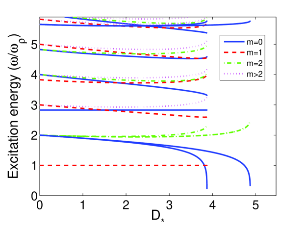
Figure 1: Excitations frequencies as function of the dipole parameter $D_{*}$ for dipolar BEC in the JILA pancake trap ($\omega_{z}/\omega_{\rho}=\sqrt{8}$), with zero scattering length. Plotted are modes with $m=0-4$. The 3 lines that extend to higher $D_{*}$ are the variational results (cf. Fig. 2 of Ref. Góral and Santos (2002)).

Let us first consider a BEC in a JILA pancake trap Jin et al. (1996) with $\frac{\omega_{z}}{\omega_{\rho}}=\sqrt{8}$. The results are presented in Fig. 1. For $D_{*}=0$ we retrieve the ideal-gas results $\frac{\omega}{\omega_{\rho}}=n_{z}\sqrt{8}+n_{\rho}$ with $n_{z},n_{\rho}=0,1,2,\ldots$. The lowest mode has $m=1$ and corresponds to a transverse Kohn mode with frequency $\omega_{\rho}$ (in fact these are two degenerate modes: m=1 and m=-1, or alternatively, sloshing motion in the $x$ and $y$ directions). The frequency is evidently constant as a function of $D_{*}$, in agreement with Kohn’s theorem. Similarly, the second lowest $m=0$ mode is a Kohn mode in the $z$ direction with frequency $\omega_{z}$. Next, consider the two modes that converge to $\omega=2\omega_{\rho}$ in the ideal-gas limit. One of them has $m=0$ (solid line) and the second $m=2$ (dashed line). The $m=0$ mode is shifted down in frequency with increasing $D_{*}$ while the $m=2$ mode is shifted up. The $m=0$ mode goes to zero at $D_{*}=3.87$. This point marks the collapse of the condensate: for higher value of $D_{*}$, there is no stable solution of the GPE. These two modes are also described by the variational method outlined above, with good agreement with the exact numerical results up to about $D_{*}=2.2$. However, the variational method significantly overestimates the $D_{*}$ for collapse (giving $D_{*}=4.87$ at collapse). Our exact numerical results are in agreement with the numerical results for these two modes obtained in Ref. Góral and Santos (2002) using the time-dependent response of the system to external perturbation, and moreover, we are able to resolve them right down to the collapse point.

The behavior of the next few low modes is also interesting: some modes of different symmetries cross each other, while two modes (one of the them the third $m=0$ mode) converge together near to collapse. Note also the 5’th $m=0$ mode, with the ideal-gas frequency of $2\omega_{z}$. This mode is also described by the variational method. We see that the lowest $m=0$ variational mode is also the lowest $m=0$ exact mode, but the second variational $m=0$ mode is much higher, and between them there are two $m=0$ modes (excluding the Kohn mode), as well as other $m>0$ modes, which are not described at all by the variational method. As mentioned above, the variational method obtains only two $m=0$ modes (excluding a Kohn mode) that approach $2\omega_{\rho}$ and $2\omega_{z}$ in the ideal gas limit. But for $\omega_{z}>2\omega_{\rho}$ there are at least two other (non-Kohn) $m=0$ modes that are between them, and approach $2\omega_{\rho}+\omega_{z}$ and $4\omega_{\rho}$ in the ideal gas limit.

It is worth noting the computational efficiency of our algorithm in obtaining these BdG results. We obtained 100 converged modes for a given dipole moment and $m$ in about half a minute on our PC, with a grid size of $N_{\rho}$x$N_{z}=$34x64.

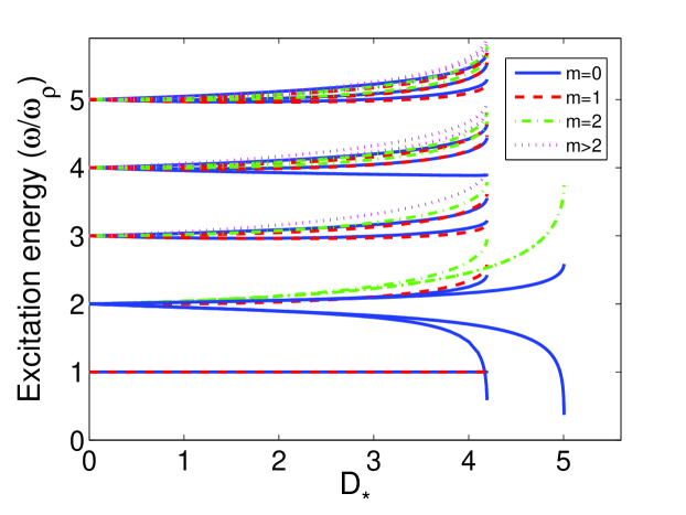
Figure 2: Excitations frequencies as function of the dipole parameter $D_{*}$ for dipolar BEC in a spherical trap with zero scattering length. Plotted are modes with $m=0-4$. The 3 lines that extend to higher $D_{*}$ are the variational results.

Let us now consider the case of a spherical trap $\omega_{\rho}=\omega_{z}\equiv\omega_{0}$, Fig. 2. The lowest excitation (in the ideal gas limit) consists of three degenerate Kohn modes corresponding to $l=1$ with $m=0,-1,+1$. Note that the Kohn frequencies are constant and maintain their degeneracy for $D_{*}>0$, even though the dipolar interaction does not conserve the total angular momentum, and the ground state shape is elongated in the $z$ direction. Next, consider the 4 modes that converge to $2\omega_{0}$: two with $m=0$, and another two with $m=1$ and $m=2$. Actually, there are six, accounting for the degeneracy with negative $m$. In the ideal gas limit these correspond to five degenerate $l=2$ modes and one $l=0$ mode. The lowest $m=0$ of these causes the collapse of the condensate at $D_{*}=4.19$. Note that this mode crosses the three Kohn modes. This is possible whenever there are two different $m$ modes or two modes with the same $m$ but different parity with respect to the symmetry $z\rightarrow-z$. The two $m=0$ modes and the $m=2$ mode are also described by the variational method. The variational frequencies agree quite well with the exact ones up to $D_{*}\approx 3$, although, again, the variational method overestimates the critical $D_{*}$ for collapse.

Note that an isotropic short range interaction that conserves $l$ would only split the degenerate ideal gas levels into different $l$ modes. Thus, if there is a dominant short range interaction and a smaller dipolar interaction in a spherical trap, the dipolar interaction would not just shift the levels, but also split them into non-degenerate states of different $|m|$. This could provide an interesting and unambiguous experimental signature of dipolar interaction effects. In such an experiment, it would be important to verify the spherical harmonicity of the trap, to exclude splitting due to anisotropy of the trap or non-harmonicity. This could be accomplished by measuring the Kohn (i.e, sloshing, or dipole) modes.

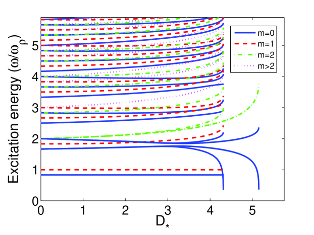
Figure 3: Excitations frequencies as function of the dipole parameter $D_{*}$ for dipolar BEC in a cigar trap with $\omega_{z}/\omega_{\rho}=5/6$ and with zero scattering length. Plotted are modes with $m=0-4$. The 3 lines that extend to higher $D_{*}$ are the variational results.

We move now to a slightly cigar shaped trap, with $\omega_{z}/\omega_{\rho}=5/6$ (Fig. 3); Here, the collapse occurs at $D_{*}=4.32$. The interesting feature here is the avoided crossing between the second and third $m=0$ modes. We find that in the avoided crossing the nature of the lowest mode changes from quadrupole-like mode for small $D_{*}$ to a breathing mode close to collapse. However, we found the same change in the nature of the lowest mode also in a spherical trap, where there is no such avoided crossings (see below. See also Góral and Santos (2002) for discussion of the nature of the modes within the variational method ).

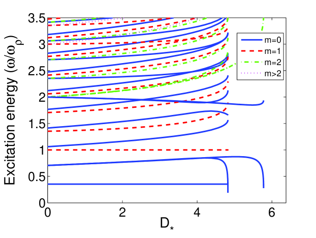
Figure 4: Excitations frequencies as function of the dipole parameter $D_{*}$ for dipolar BEC in a JILA cigar trap ($\omega_{z}/\omega_{\rho}=1/\sqrt{8}$) with zero scattering length. Plotted are modes with $m=0-4$. The 3 lines that extend to higher $D_{*}$ are the variational results (cf. Fig. 3 of Ref. Góral and Santos (2002)).

Finally, consider the JILA cigar trap Jin et al. (1996) with $\omega_{z}/\omega_{\rho}=1/\sqrt{8}$, Fig. 4. Here collapse occurs at $D_{*}=4.83$. The two $m=0$ modes which are described by the variational method have now a wide gap in energy and there is no longer a clear avoided crossing between them. There is an interesting pattern of crossing between some of the higher modes. Note again, that the lowest variational mode is the one that leads to collapse, but the two other two variational modes lie above others which are not accounted for by the variational ansatz.

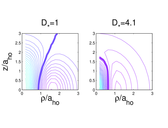
Figure 5: The spatial density perturbation $f=u+v$ (see text) for the lowest (non Kohn) mode in a spherical trap. Left: for $D_{*}=1.0$, right: for $D_{*}=4.1$, close to collapse. The nodal line is the thick line.

We can also examine the shape and nature of the BdG eigenmodes. The two eigenmode functions $u$ and $\upsilon$ are real, and determine the time dependent oscillation through Eqs. (22) and (23). The oscillation of the density $\rho(\bm{r},t)=|\psi(\bm{r},t)|^{2}$ is then given, to linear order in $u,\upsilon$, by $\delta\rho(\bm{r},t)=2(u(\bm{r})+\upsilon(\bm{r}))\cos(\omega t)$. The function $f=u+\upsilon$ therefore gives the shape of the density oscillations.

As an example, consider the lowest (non Kohn) mode in the spherical trap, the mode that goes to zero in Fig. 2 and leads to the collapse of the BEC. In Fig. 5 we draw the contour plot of $f$ for this mode, for two values of $D_{*}$, one small, and one close to the collapse point. If we examine the nodal line ($f(\bm{r})=0$, heavy line), we see that for small $D_{*}$ it forms an open, hyperbolic-like contour. This signifies a quadrupole-like mode. In contrast, close to collapse, the nodal line forms a closed, elliptic contour, typical of a breathing mode. We conclude that the nature of the mode changes from quadrupole-like for small $D_{*}$ to a breathing mode for $D_{*}$ close to collapse. This conclusion is in agreement with analysis based on the variational method Góral and Santos (2002). In between, the nodal line is parallel to the $z$ axis, and the eigenmode character is essentially that of a pure transverse ($\rho$) excitation.

IV.3 Collective versus single-particle excitations

Let us now examine in more detail the structure of the BdG excitations spectrum for a specific case. In Fig. 6 we show the spectrum evaluated for a spherical trap with $D_{*}=4$. Each state is characterized by angular momentum projection $m$, and by even (positive) parity or odd (negative) parity with respect to reflection $z\rightarrow-z$. The BdG states are represented by thick solid bars.

The BdG modes in each column of Fig. 6 are grouped in multiplets with increasing near degeneracy of $1,2,3,\ldots$ near the harmonic oscillator frequencies. In the ideal-gas limit these groups become exactly degenerate. Note that the for the $0^{+}$ column the two lowest modes (which are far apart) become degenerate (with frequency $2\omega_{0}$) at the ideal gas limit. The splitting between the groups in each given column is approximately $2\omega_{0}$. The splitting between the towers of even and odd modes of the same $m$ is approximately $\omega_{0}$. In the ideal gas limit, the tower of states with $m^{+}$ is degenerate with that of $(m-1)^{-}$. We can classify the states in the ideal gas limit by ($l,n_{r}$), with $l$ the total angular momentum, $n_{r}$ the number of radial nodes (not counting a node at $r=0$), and with energy $(2n_{r}+l)\hbar\omega_{0}$. The towers of $m^{+}$ and $(m-1)^{-}$ states become, in the ideal gas limit, a tower of $(l,n_{r})$ states as follows: the lowest state is $(l,n_{r})=(m,0)$. Above it there is a pair $(m+2,0),(m,2)$ degenerate in the ideal gas limit, followed by a triplet $(m+4,0),(m+2,2),(m,4)$ and so on. Here, the ordering of the states inside each multiplet is conventional only and does not indicate their order of increasing energy when split by the interaction.

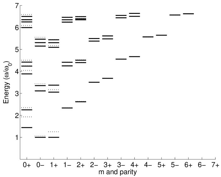
Figure 6: Excitation spectrum in a spherical trap with $D_{*}=4$. The eigenenergies of BdG equations (32) are represented by thick solid bars. Dotted bars correspond to the single-particle spectrum of the HF Hamiltonian (43).

The BdG eigenmodes are given by the pair $u,\upsilon$ corresponding to positive and negative frequencies. A collective mode is characterized by non negligible $\upsilon$ component. It describes excitation of a quasi-particle, as opposed to an excitation of a single particle. However, the high-energy part of the spectrum is expected to be well reproduced by a single-particle description in the mean-field approximation Dalfovo et al. (1997); Pitaevskii and Stringari (2003), since the condensate as a whole has little time to respond to the fast oscillations of a single particle in a high-frequency mode. The single-particle, or Hartree-Fock (HF) picture is obtained by neglecting the coupling between $u$ and $\upsilon$ in Eq. (25). This corresponds to setting $\upsilon=0$ in the first equation of Eq. (25), which then reduces to the eigenvalue problem $(H_{HF}-\mu)=\omega u$, with the HF Hamiltonian

$$H_{HF}=H_{0}+C+X.$$ (43)

In this case, the eigenfunctions $u(\bm{r})$ satisfy the normalization condition $\int u_{i}^{*}(\bm{r})u_{j}(\bm{r})=\delta_{ij}$.

The spectrum of $H_{HF}$ is shown as dotted horizontal bars in Fig. 6. The general structure of the HF spectrum is very similar to that obtained with the BdG equations (25), apart from states with low energy and $m$, which are collective modes. Note that the HF spectrum fails to satisfy the Kohn theorem for the dipole modes. It is worth noting the good agreement between the HF and the BdG spectra for $m>2$ as well as for the odd $m=1$ modes. A close look at the near-degenerate groups of the even $m=0,1$ modes shows that for the $0^{+}$ symmetry, there is good agreement between the two spectra except for two modes in each group. For the $0^{-}$ and $1^{+}$ symmetries, there is good agreement except for one mode in each group. These observations can be understood as follows. In the ideal gas limit, modes with $l>0$, have zero amplitude at the center of the condensate, where the density is at its maximum. With increasing $l$ the modes become more concentrated near the surface. The dipolar non-diagonal coupling term in Eq. (32) is proportional to the local ground state amplitude, and so becomes small for surface modes. This, assuming that modes having $l>1$ in the ideal gas limit are well approximated by the HF description, explains the pattern of Fig. 6, except for the even $m=0$ tower.

To explain the fact that for the $0^{+}$ modes we see two non single-particle modes in each near-degenerate group, we observe that, to first order of perturbation theory, the dipolar interaction mixes the $l=0$ and $l=2$ modes into two orthogonal linear combinations, each having some $l=0$ component. Thus, for example, the group of three $0^{+}$ near degenerate modes around $\omega/\omega_{0}\approx 4$ corresponds to the ideal gas modes $(l,n_{r})=(0,2),(2,1),(4,0)$. The first two are mixed already in first order of perturbation theory, so that both have some $l=0$ character, and as a consequence are not well described by the single-particle picture. This interpretation is supported by visual examination of the exact numerical eigenfunctions of the three states. Note that the state that goes to the $(4,0)$ state in the ideal gas limit is the second of the three in order of energy.

IV.4 Quantum depletion

The quantum depletion, i.e, the number of particles $\tilde{N}$ out of the condensate, due to the interaction, is given by the Bogoliubov theory as:

$$\tilde{N}=\int d\bm{r}\tilde{n}(\bm{r}),$$ (44)

with the local depletion defined by

$$\tilde{n}(\bm{r})=\sum_{j}|\upsilon_{j}(\bm{r})|^{2},$$ (45)

where the “hole” components $\upsilon_{j}$ are obtained by solving the BdG equations (32).

Typically, many thousands of modes need to be obtained in order to converge the sum in Eq. (45) Dalfovo et al. (1997). A useful approximation in this context in the local density approximation (LDA) Dalfovo et al. (1997); Reidl et al. (1999), which is the leading order of a semi-classical approximation. It was employed for the description of BEC with a repulsive short range interaction. For an attractive short range interaction, or more generally, for a dipolar BEC with $d^{2}>a/3$ Eberlein et al. (2005), an homogeneous BEC is unstable to small momentum perturbations. Thus, the LDA, which assumes local homogeneity, leads to unphysical complex frequencies for small momenta. However, it is still useful to describe the high momentum modes.

The LDA amounts to setting

$$u_{j}(\bm{r})\rightarrow u(\bm{p},\bm{r})e^{i\bm{p\cdot r}},$$

$$\upsilon_{j}(\bm{r})\rightarrow\upsilon(\bm{p},\bm{r})e^{i\bm{p\cdot r}},$$

$$\sum_{j}\cdots\rightarrow\int\frac{d^{3}\bm{p}}{(2\pi)^{3}}\cdots,$$ (46)

where $u(\bm{p},\bm{r}),\upsilon(\bm{p},\bm{r})$ are normalized by $|u(\bm{p},\bm{r})|^{2}-|\upsilon(\bm{p},\bm{r})|^{2}=1$. In the semi-classical limit the functions $u(\bm{p},\bm{r})$ and $\upsilon(\bm{p},\bm{r})$ are slowly varying on the scale of the trap size, hence their derivatives are negligible. We then obtain the same structure of the BdG equations (32), with the operators $H_{0},X$ of Eqs. (IV.1) replaced by their LDA versions:

$$H_{0}^{ld} = \frac{p^{2}}{2m}+U(\bm{r}),$$

$$(X^{ld}\chi)(\bm{p},\bm{r}) = (D_{*}\tilde{V}_{D}(\bm{p})+s)\Psi_{0}^{2}(\bm{r})\chi(\bm{p},\bm{r}),$$ (47)

where $\tilde{V}_{D}(\bm{p})$ is given by Eq. (5). The operator $C$ of Eq. (IV.1) remains unchanged, while the exchange operator $X^{ld}$ becomes local. Thus, in the LDA all the operators are local, and the solution of the BdG equations becomes algebraic. The excitation frequency is given by:

$$\omega(\bm{p},\bm{r})=\sqrt{\omega_{HF}^{2}(\bm{p},\bm{r})-X^{2}(\bm{p},\bm{r})},$$ (48)

where $\omega_{HF}$ is the HF frequency within the LDA, given by

$$\omega_{HF}(\bm{p},\bm{r})=H_{0}^{ld}(\bm{p},\bm{r})-\mu+C(\bm{r})+X^{ld}(\bm{p},\bm{r}).$$ (49)

In the semi-classical approximation, one replaces the sum over the discrete states in Eq. (45) with integral over

$$\upsilon^{2}(\bm{p},\bm{r})=\frac{\omega_{HF}(\bm{p},\bm{r})-\omega(\bm{p},\bm{r})}{2\omega(\bm{p},\bm{r})}.$$ (50)

Since the LDA is inappropriate for the low lying modes, we may calculate the contribution to Eq. (45) from exact, discrete BdG modes up to a certain frequency cutoff $\omega_{c}$, and use the LDA to obtain the contribution from higher frequency modes. Then Eq. (45) is replaced by

$$\tilde{n}(\bm{r})=\sum_{j}|\upsilon_{j}(\bm{r})|^{2}\Theta(\omega_{c}-\omega_{j})+\int_{\omega_{c}}^{\infty}d\omega\tilde{n}(\omega,\bm{r}),$$ (51)

with

$$\tilde{n}(\omega,\bm{r})=\int\frac{d\bm{p}}{(2\pi)^{3}}\upsilon^{2}(\bm{p},\bm{r})\delta(\omega(\bm{p},\bm{r})-\omega)\times$$

$$\Theta(\omega_{HF}(\bm{p},\bm{r})).$$ (52)

Note that the factor in the Dirac delta function depends on the direction in momentum space. That is, the iso-energy surfaces are not surfaces of equal momentum $p$. Also, we use the Heaviside function $\Theta(\omega_{HF}(\bm{p},\bm{r}))$ to exclude unphysical LDA modes with $\omega_{HF}<0$, even though the definition (48) can assign them a real positive frequency, due to taking the positive root. However, this matters only for small momenta below $\omega_{c}$.

As an example, we consider the case of a BEC in a spherical trap with $D_{*}$=4.0 and $s=0$. Using Eqs. (52) and (44), we find that the total depletion is 1.4 particles. The fractional depletion depends on the number of condensate particles. Since $D_{*}$ is proportional to $(N-1)d^{2}$, we can achieve the same value of $D_{*}$ with many particles with a small dipole moment, or a few particles with a large dipole moment. For the ⁵²Cr example mentioned in the beginning of section IV.2, we obtain $D_{*}=4.0$ with $N=1670$, and the quantum depletion is entirely negligible. However, we may imagine a dozen or so molecules with high dipole moment in a micro-trap. In which, case, the depletion may be measurable.

To demonstrate the agreement between the LDA and the exact BdG spectrum for high frequencies, we define the spectral distribution $g_{ld}(\omega)$ as the number of depleted bosons per unit frequency. Thus $g_{ld}(\omega)d\omega$ is the number of depleted bosons with frequency $\omega$ in the interval $d\omega$. We have

$$g_{ld}(\omega)=\int d\bm{r}\tilde{n}(\omega,\bm{r}).$$ (53)

We want to compare it with the spectral distribution $g$:

$$g(\omega)=\sum_{j}\int d\bm{r}\tilde{n}_{j}(\bm{r})\frac{1}{2\sqrt{\pi\sigma^{2}}}\exp(-\frac{1}{2}(\frac{\omega-\omega_{j}}{\sigma})^{2}),$$ (54)

obtained from the low-lying discrete modes by folding $\tilde{n}_{j}(\bm{r})$ with a Gaussian of standard deviation $\sigma$ (some smoothing of the discrete data is is necessary for meaningful comparison with the continuous LDA spectral distribution).

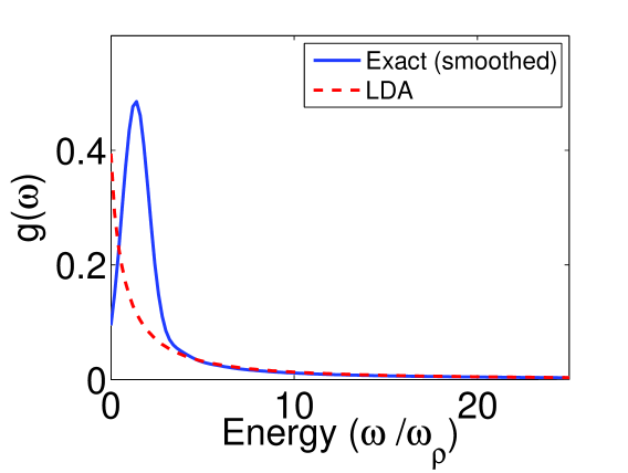
Figure 7: The spectral distribution $g_{ld}(\omega)$ in the local density approximation, Eq. (53), is compared with the smoothed, numerically exact spectral distribution $g_{(}\omega)$, Eq. (54), for BEC in a spherical trap with $D_{*}=4.0$.

In Fig. 7 we compare $g$ and $g_{ld}$ for a BEC in a spherical trap, with dipolar interaction $D_{*}=4.0$ and $s=0$. We computed $g$ from Eq. (54) with $\sigma=\omega_{0}$. For frequencies above $\omega/\omega_{0}\approx 5$ the two curves are essentially indistinguishable. This shows the efficiency of the LDA in describing the high energy part of the spectrum.

V Conclusions

We have calculated, for the first time, many BdG excited modes of a dipolar BEC in a cylindrical trap, by direct solution of of the BdG equations. This achievement was made possible by a novel, highly efficient algorithm which takes advantage of the cylindrical symmetry. We showed how properties of the BdG spectrum depend on the shape of the trap; examined in detail the spectrum in a spherical trap and the nature of the modes (collective vs single-particle); and calculated the quantum depletion due to dominant dipolar interactions, which is typically very small, but may become more significant in micro-traps containing a dozen or so molecules with high dipole moment.

We note that the formalism developed in this work may be easily extended to compute properties of dipolar BEC and its depletion at non-zero temperature using the Hartree-Fock-Bogoliubov-Popov method Reidl et al. (1999). We intend to study the non-zero temperature behavior in a future work.

*

Appendix A

A.1 Modification of the dipolar potential

In this part of the appendix we analyze the numerical accuracy of the 3D FFT method for calculating the dipolar interaction. A correction is suggested to increase the accuracy, and this correction also applies to our 2D algorithm.

The 3D FFT method was used to calculate the mean field potential due to dipolar interactions via Eq. (4). To check its accuracy it is more convenient to consider the dipolar interaction energy for a dipole strength $D_{*}=1$, given by:

$$E_{D}=\frac{1}{2}\int\int d\bm{r}d\bm{r^{\prime}}V_{D}(\bm{r}-\bm{r^{\prime}})n(\bm{r^{\prime}})n(\bm{r}).$$ (55)

Given $n(\bm{r})$, this expression can be evaluated numerically on a 3D grid by first performing the $\bm{r^{\prime}}$ integration using Eq. (4), which requires FFT and inverse FFT, and then performing the $\bm{r}$ integration as discrete summation on the spatial grid. Note that $\tilde{V}_{D}(k)$ in Eq. (4) is given analytically by Eq. (5) and does not require FFT.

Eq. (55) may be alternatively written in the form:

$$E_{D}=\frac{1}{2(2\pi^{3})}\int d\bm{k}\tilde{V}_{D}(k)\tilde{n}(\bm{k})^{2}.$$ (56)

This expression may be evaluated numerically by using one FFT to obtain $\tilde{n}(k)$ and then performing the integration as summation in momentum space. The two numerical procedures give the same result up to machine precision.

For a Gaussian density

$$n(\bm{r})=\frac{1}{\pi^{3/2}\sigma^{2}\sigma_{z}}\exp(-(x^{2}+y^{2})/\sigma^{2}-z^{2}/\sigma_{z}^{2})$$ (57)

it is possible to obtain an analytic expression for $E_{D}$ using Eq. (56) Martikainen et al. (2002); Yi and You (2000). This enables us to check the accuracy of the numerical calculation.

For a spherically symmetric Gaussian, $\sigma=\sigma_{z}$, defined on a cubic grid with equal resolution in the three axis, we find numerically the exact result $E_{D}=0$. In fact, by noticing that $\tilde{V}_{D}(k)=\frac{4\pi}{3}\frac{2k_{z}^{2}-k_{x}^{2}-k_{y}^{2}}{k^{2}}$, it is seen that $E_{D}$ evaluated on a cubic grid is guaranteed to be zero for any density $n(x,y,z)$ which is symmetric under all permutations of $(x,y,z)$.

For a pancake shaped density $\sigma=2,\sigma_{z}=1$, the exact result is $E_{D}=0.038670861\ldots$. We have evaluated it on cubic grids of extent $[-R,R]\times[-R,R]\times[-R,R]$ with varying size $R$ and number of points $N$x$N$x$N$ . The relative error is tabulated in the first row of table 1. It is seen that the errors are small but far from machine accuracy. Note that convergence with respect to $N$ is already achieved with a modest spatial resolution of $2R/N=2*8/32=0.5$, but there is a rather slow convergence with increasing $R$. This make it clear that the error is not due to failure to resolve the density function $n(r)$. For cigar shaped densities similar behavior was observed.

Table 1: Relative error of evaluating dipolar interaction energy using the 3D FFT method, before and after correction, for a pancake Gaussian density (see text).

	$R=8,N=32$	$R=8,N=64$	$R=16,N=64$	$R=16,N=128$
original method	2.7E-3	2.7E-3	8.6E-5	8.6E-5
corrected method	-1.1E-5	-1.1E-5	1.8E-8	-4.4E-14

The reason for the behavior of the numerical error is understood if we realize that $\tilde{V}_{D}(k)$ is discontinuous at the origin, where $n(k)$ obtains its maximum. This discontinuity originates in the long range and non-isotropic nature of the interaction. Thus, the numerical accuracy converges slowly with increasing grid resolution, proportional to $1/R$, in momentum space.

An alternative and equivalent way to understand the source of the error is that the use of FFT implicitly assumes that we are dealing with a 3D periodic lattice of condensates, with unit cell of size $2R$. Thus the error may be traced down to the long range interactions between copies of condensates in different unit cells.

An obvious correction suggests itself: since our actual condensate is isolated and of a finite size, we can limit the range of the dipolar interaction $V_{D}(r)$ such that it is the same as before for $r<R$ and and zero for $r\geq R$. This should have no physical consequences as long as $R$ is greater than the extent of our condensate. Then the Fourier transform of this interaction is continuous at the origin and resolved by the grid in momentum space. We obtain the following expression for the corrected dipolar interaction $\tilde{V}_{D}^{cutR}(k)$:

$$\tilde{V}_{D}^{cutR}(\bm{k}) = \frac{4\pi}{3}(1+3\frac{\cos(Rk)}{R^{2}k^{2}}-3\frac{\sin(Rk)}{R^{3}k^{3}})\times$$ (58)

$$(3\cos^{2}\alpha-1).$$

Using this corrected interaction, we obtain the much better accuracy demonstrated in the second line of table 1. The remaining error depends on $R$ only due to the spatial extent of the condensate, and fast convergence is achieved by increasing $R$ while keeping appropriate grid resolution through increasing $N$. One may compromise on $R$ and $N$, and still obtain at least a 100 fold increase in accuracy as compared to using the infinite range interaction.

For highly pancake/cigar traps the condensate has also a highly pancake/cigar shape. In this case it is natural to work with a grid whose extent $[-Z,Z]$ in the $z$ direction is, respectively, smaller/larger than its extent $[-P,P]\times[-P,P]$ in the $(x,y)$ plane. Thus, fewer grid points are needed along the shorter axis. In this case, we find that without correction, numerical errors can be typically as large as one percent. However, truncating the interaction outside a sphere as in Eq. (58) is not very helpful in this case, since the condition $R\leq\min(Z,P)$ must be met, which restricts the condensate extent to less than the shorter direction. The ideal fix would be to cut the interaction exactly by the shape of the box, or a cylinder inscribed within it. We were unable to find an analytic expression for the Fourier transform of a dipolar interaction bounded by a cylinder. A partial but still helpful solution for pancake traps is to truncate the interaction only for $|z|>Z$. We then find:

$$V_{D}^{cutZ}(\bm{k})=$$ (59)

$$\frac{4\pi}{3}(3\cos^{2}\alpha-1)+4\pi\exp(-Zk_{\rho})\Big{[}\sin^{2}\alpha\cos(Zk_{z})-$$

$$\sin\alpha\cos\alpha\sin(Zk_{z})\Big{]}.$$

With this corrected interaction, a small $Z$ may be used as long as it fully contains the condensate. Numerical convergence with the size $P$ will still be slow, but typically the accuracy is improved by an order of magnitude at the least.

Finally, with our 2D algorithm combining Hankel transform in the transverse direction and Fourier transform in the $z$ direction, we find numerical errors of similar behavior and magnitude. In the case of 2D, small numerical errors exists even for a spherical symmetric density, since there is no symmetry of the grid that ensures getting the correct zero energy, as in the 3D case. All of these errors are significantly reduced by employing the same cutoff interactions as in the 3D case.

A.2 Conjugate-gradients implementation

We describe here in some detail aspects of the conjugate-gradients implementation specific to the problem of finding the ground state of a dipolar condensate, see section III.The standard conjugate-gradients algorithm performs unconstrained minimization. In principle a constraint could be implemented through a Lagrange multiplier. In our implementation we rather follow the idea of Modugno et al. (2003). To account more easily for the normalization constraint, Eq. (21), we let $\Psi\rightarrow\Psi/\|\Psi\|$ so that the energy can be obtained for condensate wave functions $\Psi$ with a norm different from unity. This corresponds to dividing the terms of $E[\Psi,\Psi^{*}]$ in Eq. (19) that are quadratic in $\Psi$ by $\|\Psi\|^{2}$, and the interaction term quartic in $\Psi$ by $\|\Psi\|^{4}$. The modified energy functional reads:

$$E[\Psi,\Psi^{*}]=$$ (60)

$$\int d\bm{r}\frac{\Psi^{*}(\bm{r})H_{0}\Psi(\bm{r})}{\|\Psi\|^{2}}+$$

$$\frac{N-1}{2\|\Psi\|^{4}}\int\int d\bm{r}d\bm{r^{\prime}}|\Psi^{2}(\bm{r^{\prime}})|V(\bm{r}-\bm{r^{\prime}})|\Psi^{2}(\bm{r})|.$$

This functional may now be minimized directly with no constraints. During the minimization process it may still be numerically advantageous to normalize the wavefunction at each step.

One ingredient of the conjugate-gradients method is a line minimization of the energy functional, that is the minimization of

$$E(\Psi_{0}+\lambda\chi)$$ (61)

with respect to $\lambda$, where $\Psi_{0}$ is the current trial wavefunction and $\chi$ is the proposed direction along which to move. An important issue for our specific problem is to find the first minimum encountered when moving downhill in energy along the line: whenever $d^{2}>a/3$, the global minimum is a collapsed state Yi and You (2000), while the condensate corresponds to a stable local minimum (if such exists). Therefore, it is important that the line minimization will not jump to an energy valley leading to the global one, but stay in the energy valley of the initial guess. This issue is usually not considered as important in the textbook implementation of the conjugate-gradients method. Following Modugno et al. (2003) we use the fact that the Eq. (61) is a rational function of $\lambda$. We then easily find the roots of $dE/d\lambda$ and the first local minimum of $E$ encountered when one moves along the line downhill in energy starting from $\lambda=0$. The coefficients of the numerator in the rational function require calculation of dipolar interaction integrals with combinations of $\Psi$ and $\chi$ such as $\int\int d\bm{r}d\bm{r^{\prime}}\Psi(\bm{r})\chi(\bm{r})V_{D}(\bm{r}-\bm{r^{\prime}})\chi^{2}(\bm{r^{\prime}})$, etc. These integrals can be computed in momentum space by using DHFT and the identity:

$$\int\int d\bm{r}d\bm{r^{\prime}}n_{1}(\bm{r})V_{D}(\bm{r}-\bm{r^{\prime}})n_{2}(\bm{r^{\prime}})=$$ (62)

$$\frac{1}{(2\pi)^{3}}\int d\bm{k}\tilde{n}_{1}(\bm{k})\tilde{V}_{D}(\bm{k})\tilde{n}_{2}(\bm{k}).$$

After finding the local minimum along a given line we proceed with another line minimization along a conjugate direction, and so forth until we find a local minimum of the energy functional Eq. (60).

An additional technical ingredient in our implementation of the conjugate-gradients algorithm is the use of pre-conditioning Payne et al. (1992), a technique used to accelerate the convergence. Our pre-conditioner is given in momentum space as $\frac{1}{k^{2}/2+M}$, with $M=\max(E,E_{k})$, $E$ is the energy given by Eq. (60), and $E_{k}$ is the kinetic energy.

A.3 Excitations spectrum

An important issue in calculating the $m>0$ excitations is that the grid points given by Eq. (9) are different for different $m$. The point is that the function $f$ of Eq. (41a) is represented on the $m>0$ grid, whereas the ground state wavefunction entering Eqs. (IV.1), is defined on the $m=0$ grid. Our solution is to interpolate the ground state wavefunction to the grid $m>0$. The interpolation is facilitated by the fact that the roots of the Bessel function $J_{m}(r)$ march to the right as $m$ is increased, and those of $m$ are interlaced between those of order $m-1$. Fortunately, a highly accurate interpolation scheme is available in this case Makowski (1982). Similarly to the exact integration formula (16), one can derive an exact interpolation formula for band limited functions satisfying Eq. (15):

$$f(r)=\sum_{i=1}^{\infty}\frac{2\alpha_{0i}J_{0}(2\pi Kr)}{(\alpha_{0i}^{2}-(2\pi Kr)^{2})}\frac{f(r_{i})}{J_{1}(\alpha_{0i})},$$ (63)

with the grid points $r_{i}=\frac{\alpha_{0i}}{2\pi K}$. This formula may be proved by writing $f(r)$ as the Hankel transform (of order $0$) of $\tilde{f}(k)$. Expanding $\tilde{f}(k)$ in a Fourier-Bessel series, the coefficients are found to be proportional to $f(r_{i})$. Evaluating the resulting expression gives Eq. (63). This formula, exact for band limited functions, still gives very accurate approximation for $f(r)$ such that its Hankel transform (i.e, its 2D Fourier transform) is small for $k>K$. It can be truncated to the first $N$ terms provided $f(r)$ is small for $r\geq R=\alpha_{0,i+1}/K$. We used this formula to interpolate the ground state wavefunction to the required grid points of $m>0$. Note that this interpolation need only be done once prior to solving the BdG eigensystem. An alternative method for calculating $m>0$ modes using a fixed grid corresponding to $m=0$ with no need for interpolation was suggested in Refs. Lemoine (1994b, 1997).

In our application we have taken advantage of the structure of the BdG equations (section IV) to efficiently compute the low lying spectrum. We have used a variant of the Arnoldi method (the implicitly restarted Arnoldi method), which is implemented in the ARPACK software package , and enables finding the $M$ largest or smallest eigenvalues of an operator $\bm{A}$, where $M$ is selected by the user. $\bm{A}$ need not be hermitian. For our purposes, the main advantage of this method is that it requires as input only the evaluation of $\bm{A}$$x$ for some vector $x$. The matrix elements of $\bm{A}$ need not be known. The user need only provide a function that accepts $x$ and returns $y=\bm{A}x$. The eigenvalues in the requested part of the spectrum are then found iteratively by repeated applications of $A$, starting from some randomly chosen $x$. In our case, $Ax$ represents the l.h.s of Eq. (41a), and the computation is facilitated, as usual, by using DHFT to move between space and momentum space representations.

References

- Stuhler et al. (2005) J. Stuhler, A. Griesmaier, T. Koch, M. Fattori, T. Pfau, S. Giovanazzi, P. Pedri, and L. Santos, Phys. Rev. Lett. 95, 150406 (2005).
- Yi and You (2000) S. Yi and L. You, Phys. Rev. A 61, 041604 (2000).
- Góral et al. (2000) K. Góral, K. Rza̧żewski, and T. Pfau, Phys. Rev. A 61, 051601 (2000).
- Yi and You (2001) S. Yi and L. You, Phys. Rev. A 63, 053607 (2001).
- Yi and You (2002) S. Yi and L. You, Phys. Rev. A 66, 013607 (2002).
- Baranov et al. (2002) M. Baranov, L. Dobrek, K. Góral, L. Santos, and M. Lewenstein, Phys. Scr. T102, 74 (2002).
- Góral and Santos (2002) K. Góral and L. Santos, Phys. Rev. A 66, 023613 (2002).
- Santos et al. (2003) L. Santos, G. V. Shlyapnikov, and M. Lewenstein, Phys. Rev. Lett. 90, 250403 (2003).
- O’Dell et al. (2004) D. H. J. O’Dell, S. Giovanazzi, and C. Eberlein, Phys. Rev. Lett. 92, 250401 (2004).
- Nho and Landau (2005) K. Nho and D. P. Landau, 023615, 023615 (2005).
- Cooper et al. (2005) N. R. Cooper, E. H. Rezayi, and S. H. Simon, Phys. Rev. Lett. 11, 200402 (2005).
- Bortolotti et al. (2006) D. C. E. Bortolotti, S. Ronen, J. L. Bohn, and D. Blume, cond-mat/0604432 (2006).
- Ronen et al. (2006) S. Ronen, D. C. E. Bortolotti, D. Blume, and J. L. Bohn, cond-mat/0605315 (2006).
- Arfken and Weber (2001) G. B. Arfken and H. J. Weber, Mathematical Methods for Physicists (Harcourt: San Diego, 2001), 5th ed.
- Siegman (1977) A. E. Siegman, Opt. Lett. 1, 13 (1977).
- Talman (1978) J. D. Talman, J. Comp. Phys. 29, 35 (1978).
- Hamilton (2000) A. J. S. Hamilton, MNRAS 312, 257 (2000).
- Bisseling and Kosloff (1985) R. Bisseling and R. Kosloff, J. Comp. Phys. 59, 136 (1985).
- Yu et al. (1998) L. Yu, M. Huang, M. Chen, W. Chen, W. Huang, and Z.Zhu, Opt. Lett. 23 23, 409 (1998).
- Guizar-Siciaros and Gutiérrez-Vega (2004) M. Guizar-Siciaros and J. C. Gutiérrez-Vega, 21, 53 (2004).
- Lemoine (1994a) D. Lemoine, J. Chem. Phys. 101, 3936 (1994a).
- Lemoine (1997) D. Lemoine, Comp. Phys. Comm. 99, 297 (1997).
- Lemoine (2003) D. Lemoine, J. Chem. Phys. 118, 697 (2003).
- Frappier and Olivier (1993) C. Frappier and P. Olivier, Mathematics of Computation 60, 303 (1993).
- R.Grozev (1995) G. R.Grozev, Mathematics of Computation 64, 715 (1995).
- Ogata (2005) H. Ogata, Publications of the Research Institute for Mathematical Sciences 41, 949 (2005).
- Press et al. (1992) W. H. Press, B. P. Flannery, S. A. Teukolsky, and W. T. Vetterling, Numerical Recipes in C: The Art of Scientific Computing (Cambridge University Press, 1992), 2nd ed.
- Payne et al. (1992) M. C. Payne, M. P. Teter, D. C. Allan, T. A. Arias, and J. D. Joannopoulos, Rev. Mod. Phys. 64, 1045 (1992).
- Modugno et al. (2003) M. Modugno, L. Pricoupenko, and Y. Castin, Eur. Phys. J. D 22, 235 (2003).
- Pitaevskii and Stringari (2003) L. P. Pitaevskii and S. Stringari, Bose-Einstein Condensation (Oxford University Press, New York, 2003).
- Huepe et al. (2003) C. Huepe, L. S. Tuckerman, S. Métens, and M. E. Brachet, Phys. Rev. A 68, 023609 (2003).
- Arnoldi (1951) W. E. Arnoldi, Q. Appl. Math. 9, 17 (1951).
- Ruprecht et al. (1996) P. A. Ruprecht, M. Edwards, K. Burnett, and C. W. Clark, Phys. Rev. A 54, 4178 (1996).
- Pérez-García et al. (1996) V. M. Pérez-García, H. Michinel, J. I. Cirac, M. Lewenstein, and P. Zoller, Phys. Rev. Lett. 77, 5320 (1996).
- Kohn (1961) W. Kohn, 123, 1242 (1961).
- Werner et al. (2005) J. Werner, A. Griesmaier, S. Hensler, J. Stuhler, T. Pfau, A. Simoni, and E. Tiesinga, Phys. Rev. Lett. 94, 183201 (2005).
- Pavlović et al. (2005) Z. Pavlović, R. V. Krems, R. Côté, and H. R. Sadeghpour, Phys. Rev. A 71, 061402 (2005).
- Jin et al. (1996) D. S. Jin, J. R. Ensher, M. R. Matthews, C. E. Wieman, and E. A. Cornell, Phys. Rev. Lett. 77, 420 (1996).
- Dalfovo et al. (1997) F. Dalfovo, S. Giorgini, M. Guilleumas, L. Pitaevskii, and S. Stringari, Phys. Rev. A 56, 3840 (1997).
- Reidl et al. (1999) J. Reidl, A. Scordás, R. Graham, and P. Szépfalusy, Phys. Rev. A 59, 3816 (1999).
- Eberlein et al. (2005) C. Eberlein, S. Giovanazzi, and D. H. J. O’Dell, Phys. Rev. A 71, 033618 (2005).
- Martikainen et al. (2002) J. P. Martikainen, M. Mackie, and K. A. Suominen, Phys. Rev. A 64, 037601 (2002).
- Makowski (1982) L. Makowski, J. App. Cryst. 15, 546 (1982).
- Lemoine (1994b) D. Lemoine, Chem. Phys. Lett. 224, 483 (1994b).