Absence of extended states in a ladder model of DNA

Abstract

We consider a ladder model of DNA for describing carrier transport in a fully coherent regime through finite segments. A single orbital is associated to each base, and both interstrand and intrastrand overlaps are considered within the nearest-neighbor approximation. Conduction through the sugar-phosphate backbone is neglected. We study analytically and numerically the spatial extend of the corresponding states by means of the Landauer and Lyapunov exponents. We conclude that intrinsic-DNA correlations, arising from the natural base pairing, does not suffice to observe extended states, in contrast to previous claims.

I Introduction

According to standard theories of disordered systems, Abrahams79 all states in low-dimensional systems with uncorrelated disorder are spatially localized. Therefore, in a pure quantum-mechanical regime, DNA might be insulator unless the localization length reaches anomalously large values. To explain long range electronic transport found experimentally, Porath00 Caetano and Schulz claimed that intrinsic DNA-correlations, due to the base pairing (A–T and C–G), lead to electron delocalization. Caetano05 Furthermore, they pointed out that there is a localization-delocalization transition (LDT) for certain parameters range. If these results were correct, then transverse correlations arising intrinsically in DNA could explain long range electronic transport. However, we have claimed that this is not the case and all states remain localized, thus excluding a LDT. Sedrakyan06 Therefore, the electrical conduction of DNA at low temperature is still an open question.

In this paper we provide further analytical and numerical support to our above mentioned claim, aiming to understand the role of intrinsic DNA-correlations in electronic transport. To this end, we address signatures of the spatial extend of the electronic states by means of the analysis of the Landauer and Lyapunov coefficients, to be defined below. The outline of the paper is as follows. In the next section, we introduce the ladder model of DNA Caetano05 and diagnostic tools we use to elucidate the spatial extend of electronic states in the static lattice. In Sec. III we discuss the analytical calculation of the Landauer exponent and show that this exponent never vanishes in the thermodynamics limit for any value of the system parameters. From this result we conclude that extended states never arise in the model. We then proceed to Sec. IV, in which we numericaly calculate the Lyapunov exponent for finite samples. We discuss in detail its dependence on the model parameters, especially inter- and intrastrand hoppings. We provide evidences that the localization length is only of the order of very few turns of the double helix for realistic values of the model parameters. Therefore, this shows that intrinsic DNA-correlations alone cannot explain long range electronic transport. found in long DNA molecules. Porath00 Finally, Sec. V concludes the paper.

II Model and diagnostic tools

Our analysis proceeds as follows. We consider a ladder model of DNA in a fully coherent regime and assign a single orbital to each base. Conduction through the sugar-phosphate backbone is neglected hereafter. Both interstrand and intrastrand overlaps are considered within the nearest-neighbor approximation. We assume that the hopping does not depend on the base and therefore only two values are considered, namely interstrand ($t_{\perp}$) and intrastrand ($t_{\|}$) hoppings. Figure 1 shows a schematic view of a fragment of this ladder model.

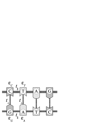
Figure 1: Schematic view of a fragment of the ladder model for DNA molecules, excluding the sugar-phosphate backbone. A single orbital is associated to each base, with a corresponding energy $\varepsilon_{n}$, $n$ being A, T, C or G. The sequence of the basis of one of the strands is random, while the sequence of the other strand results from the base pairing A–T and C–G. Only two different hoppings are considered, namely interstrand ($t_{\perp}$) and intrastrand ($t_{\|}$) hoppings.

Four different values of the energy sites ($\varepsilon_{A}$, $\varepsilon_{T}$, $\varepsilon_{C}$, and $\varepsilon_{G}$) are randomly assigned in one of the strands, with the same probability, while the sites of the second strand are set to follow the DNA pairing (A–T and C–G). Hereafter we will restrict ourselves to the following values of the site energies, taken from Ref. Roche03, , $\varepsilon_{A}=8.24\,$eV, $\varepsilon_{T}=9.14\,$eV, $\varepsilon_{C}=8.87\,$eV, $\varepsilon_{G}=7.75\,$eV. The same site energy values were taken in Ref. Caetano05, . As a consequence, only three parameters remain in the model, namely $t_{\perp}$, $t_{\|}$ and $N$, the number of base pairs. We will show below that the spatial extend of the states strongly depends on $t_{\perp}$ and $t_{\|}$, but never goes to infinity in the thermodynamics limit ($N\to\infty$).

Once the model has been established, we can write down the equation for the amplitudes at different bases. Let us denote these amplitudes as $\psi_{n}^{(\sigma)}$, where $\sigma=1,2$ runs over the two strands and $n=1,2,\ldots,N$ denotes the position of the bases at each strand. According to the model introduced above, the equations for the amplitudes are readily found to be

$$E\psi_{n}^{(1)}=\varepsilon_{n}^{(1)}\psi_{n}^{(1)}+t_{\|}\left(\psi_{n+1}^{(1)}+\psi_{n-1}^{(1)}\right)+t_{\perp}\psi_{n}^{(2)}\ ,$$ (1a)

$$E\psi_{n}^{(2)}=\varepsilon_{n}^{(2)}\psi_{n}^{(2)}+t_{\|}\left(\psi_{n+1}^{(2)}+\psi_{n-1}^{(2)}\right)+t_{\perp}\psi_{n}^{(1)}\ .$$ (1b)

Here $\varepsilon_{n}^{(\sigma)}$ takes one of the four values of the site energies, according to the constraints presented above.

The equation for the amplitudes can be cast in a compact form by using $4\times 4$ transfer matrices. To this end, let us introduce the $4$-vector

$${\bm{\Phi}}_{n}\equiv\left(\psi_{n}^{(1)},\psi_{n}^{(2)},\psi_{n-1}^{(1)},\psi_{n-1}^{(2)}\right)^{t}$$ (2a)

where the superscript $$t 2\times 2$$ indicates the transpose. Defining the following matrix

$$M_{2}^{(n)}\equiv\left(\begin{array}[]{cc}\frac{E-\varepsilon_{n}^{(1)}}{t_{\|}}&-\,\frac{t_{\perp}}{t_{\|}}\\ -\,\frac{t_{\perp}}{t_{\|}}&\frac{E-\varepsilon_{n}^{(2)}}{t_{\|}}\end{array}\right)\ ,$$ (2b)

we arrive at the transfer-matrix equation $${\bm{\Phi}}_{n+1}=T_{n}{\bm{\Phi}}_{n}$$, with

$$T_{n}\equiv\left(\begin{array}[]{cc}M_{2}^{(n)}&-\mathcal{I}_{2}\\ \mathcal{I}_{2}&\mathcal{O}_{2}\end{array}\right)\ ,$$ (2c)

where $\mathcal{I}_{2}$ and $\mathcal{O}_{2}$ are the unity and null $2\times 2$ matrices, respectively. One can easily find out, that the $4\times 4$ transfer matrix $T_{n}$ satisfies the condition $T_{n}^{\dagger}JT_{n}=J$ with

$$J=\left(\begin{array}[]{cccc}0&0&-i&0\\ 0&0&0&-i\\ i&0&0&0\\ 0&i&0&0\end{array}\right)$$ (7)

which means that $T_{n}$ belong to the $SU(2,2)$ group. It is to be noticed that only four transfer matrices appear in DNA due to the intrinsic pairing (see Fig. 1), and they will be denoted as $T_{n,AT}$, $T_{n,TA}$, $T_{n,CG}$, $T_{n,GC}$ for the sake of clarity.

The electronic properties can be described by the full transfer matrix ${\cal M}_{N}=\prod_{n=N}T_{n,ij}$ and the Lyapunov exponents, $\gamma_{\textrm{Ly}}$, the eigenvalues of the limiting matrix $\lim_{N\to\infty}\,\ln({\cal M}_{N}{\cal M}_{N}^{\dagger})^{1/2N}$, provide information about the localization length of the states, assuming exponential localization.Kramer93 Here $i,j\in\{\mathrm{A,T,G,C}\}$ and length is measured in units of the base separation along a single strand ($3.1\,$nm). Due to the self-averaging property they can be calculated by taking the product of random transfer matrices over a long system. Similarly, in the Landauer exponent $\gamma_{\textrm{La}}(N)=\ln\langle\,||\prod_{n=N}^{1}T_{n,ij}||\,\rangle^{1/N}$ (hereafter $\langle\ldots\rangle$ denotes ensemble averages) is twice the largest Lyapunov exponent near the critical region in one-dimensional systems Anderson80 ; SSBS and can be calculated analytically following the technique developed in Refs. Sedrakyan99, ; Hakobyan00, ; Sedrakyan04, . In quasi-one dimensional chains, as in the ladder system under consideration, both exponents again exhibit the same critical behavior (the critical indices are the same), but their ratio can be different from 2.

III Landauer exponent

In Refs. Sedrakyan99, ; Hakobyan00, ; Sedrakyan04, it was shown that the Landauer resistance and the corresponding exponent can be calculated exactly. To this end, the direct product ${\cal M}_{N}\otimes{\cal M}_{N}^{\dagger}$ of the fundamental representations of transfer matrices of the $SU(1,1)$ group is reduced to the adjoint one. We apply this technique here for the group $SU(2,2)$. In order to calculate this direct product exactly, we use the known representation of the permutation operator via generators $\tau^{\mu}$ $(\mu=1,\dots,15)$ of the $sl(4)$ algebra as $P=(1/4)(\mathbb{I}\otimes\mathbb{I}+\tau^{\mu}\otimes\tau^{\mu})$. Thus the matrix elements satisfy

$$\delta_{\alpha_{1}}^{\alpha_{2}}\delta_{\beta_{1}}^{\beta_{2}}=\frac{1}{4}\,[\delta_{\alpha_{1}}^{\beta_{2}}\delta_{\beta_{1}}^{\alpha_{2}}+(\tau^{\mu})_{\alpha_{1}}^{\beta_{2}}(\tau_{\mu})_{\beta_{1}}^{\alpha_{2}}]\ ,$$ (8)

where we assume summation in the repeated indices $\mu$. Among of generators $\tau^{\mu}$ there is one, which coincides with the metric $J$ defined in (7). We denote the corresponding index $\mu$ as $J$, namely $\tau^{J}=J$.

Multiplying (8) by $T_{j}$ and $T^{\dagger}_{j}$ from the left and right hand sides respectively, one can express the direct product of $T_{j}$ and $T^{\dagger}_{j}$ via their adjoint representation

$$(T_{j})^{\alpha}_{\alpha^{\prime}}(T_{j}^{+})^{\beta^{\prime}}_{\beta}={\frac{1}{4}}(J)^{\alpha}_{\beta}(J)^{\beta^{\prime}}_{\alpha^{\prime}}+{\frac{1}{4}}(\tau^{\mu}J)^{\beta^{\prime}}_{\alpha^{\prime}}\Lambda_{j}^{\mu\nu}(J\tau^{\nu})^{\alpha}_{\beta}\ .$$ (9)

Here the adjoint representation $\Lambda_{n}$ of $T_{n}$ is defined by

$$\Lambda_{n}^{\mu\nu}=\frac{1}{4}{\rm Tr}(T_{n}\tau^{\mu}T^{+}_{n}\tau^{\nu})\ ,$$ (10)

being an $15\times 15$ matrix that depends on the parameters of the model at site $n$ of both chains.

To calculate analytically the Landauer exponent, we apply this decomposition to the products of fundamental representations, $T_{n}$’s in ${\cal M}_{N}$, and after averaging obtain

$$\langle{\cal M}_{N}{\cal M}_{N}^{\dagger}\rangle={\frac{1}{4}}J\otimes J+{\frac{1}{4}}(\tau^{\mu}J)\otimes(J\tau^{\nu})\left(\prod_{j=1}^{N}\langle\Lambda_{j}\rangle\right)^{\mu\nu}\ .$$ (11)

It is then straightforward to get the average over four equivalent substitutions of the base pairs in the random chain

$$\langle\Lambda^{\mu\nu}\rangle=\frac{1}{4}\,\left(\Lambda^{\mu\nu}_{AT}+\Lambda^{\mu\nu}_{TA}+\Lambda^{\mu\nu}_{CG}+\Lambda^{\mu\nu}_{GC}\right)\ .$$ (12)

The Landauer exponents are the nonnegative eigenvalues of $\frac{1}{2}\log\langle\Lambda\rangle$. The condition of the existence of an extended state is equivalent to $\det|\langle\Lambda\rangle-I|=0$, and it is a matter of simple algebra to prove that this condition is never met.

Therefore, we come to the conclusion that the system studied by Caetano and Schulz Caetano05 cannot support truly extended states. Consequently, a LDT is not to be observed since all states are spatially localized.

IV Lyapunov exponent

It can be argued that, although the localization length is always finite, as we have demonstrated above, it could be larger than typical sizes used in transport experiments, as those carried out by Porath et al. Porath00 To quantitatively determine the spatial extend of the electronic states, we have numerically calculated the Lyapunov exponents for different values of the hoppings $t_{\perp}$ and $t_{\|}$.

Figure 2 shows the Landauer and Lyapunov exponents for $N=4000$, when $t_{\perp}=0.5\,$eV and $t_{\|}=1.0\,$eV. These values of the interstrand and intrastrand hoppings are larger than those usually considered in the literature, Yan02 ; Klotsa05 but they were used by Caetano and Schulz Caetano05 to provide support to their claim about the extended nature of the states. From Fig. 2 it becomes clear that neither the largest Lyapunov exponents nor the Landauer one vanish over the whole energy spectrum. Most important, its minimum value is size independent within the numerical accuracy, suggesting the occurrence of truly localized states. Notice that the minimum value of these exponents is always much larger than the inverse of the number of base pairs ($1/N=0,00025$), indicating that DNA-pairing can hardly explain long range charge transport at low temperature. From the inverse of the minimum value of the second Lyapunov coefficient we can estimate that the localization length is of the order of $80$ base pairs (i.e. roughly eight turns of the double helix), therefore being much smaller than typical sizes used in experiments. Porath00

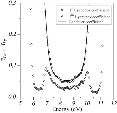
Figure 2: $2/3$ of Landauer exponent $\gamma_{\mathrm{La}}$ (solid line) and the largest Lyapunov exponent $\gamma_{\mathrm{Ly}}$ (white circles), as a function of energy, for $t_{\perp}=0.5\,$eV and $t_{\|}=1.0\,$eV. The second, smaller Lyapunov exponent (grey circles) is also shown.

To elucidate the effects of the base pairing on the localization length, we have also considered the artificial case of ladder models without pairing. In that case, both strands are completely random, allowing for a larger number of possible pairs (e.g. AC or AA). Therefore, the system becomes much more disordered and one could naively expect a dramatic decrease of the localization length, as compared to the system with base pairing. Figure 3 indicates that this is not the case. The inverse of the second Lyapunov exponent remains almost unchanged over a large region of the energy spectrum, except close to the two resonances at about $6.4\,$eV and $10.6\,$eV. At resonances the localization length is reduced by a factor $2.5$ at most when the pairing constraint is relaxed. In any event, resonances still appear so they cannot be associated to base pairing.

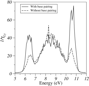
Figure 3: Inverse of the second Lyapunov coefficient for $N=4000$ $t_{\perp}=0.5\,$eV and $t_{\|}=1.0\,$eV, when the base pairing is present (solid line) and absent (dashed line).

We claimed that the spatial extend of states strongly depends on the hopping parameters, Sedrakyan06 and those considered in Ref. Caetano05, seems to be larger as compared to those values widely admitted in the literature. Yan02 ; Klotsa05 Higher hoppings lead to a less-effective disorder and higher localization lengths are to be expected. We have calculated the inverse of the second Lyapunov exponent for more realistic values of the hopping parameter and checked that this claim is indeed correct. For instance, for $t_{\perp}=0.05\,$eV and $t_{\|}=0.5\,$eV (see Ref. Klotsa05, ) the localization length at the center of the band is reduced by a factor $5$ as compared to the case shown in Fig. 1, while an even larger decrease is noticed at resonances. Therefore, we come to the conclusion that hopping is more important than base-pairing in this ladder model.

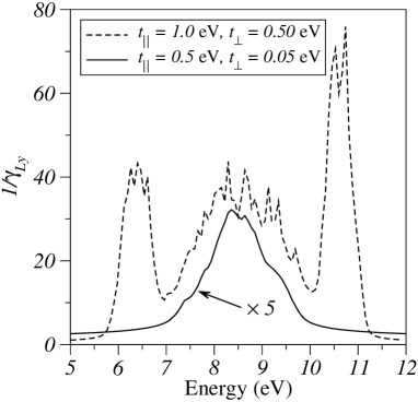
Figure 4: Inverse of the second Lyapunov coefficient for $N=4000$ and two sets of hopping parameters, indicated on the legend box. Notice the scaling factor indicated on the lower curve.

V Conclusions

We considered a ladder model of DNA for describing electronic transport in a fully quantum-mechanical regime. In this model, a single orbital is assigned to each base, and the sugar-phosphate channels are excluded. Therefore, it is assumed that electronic conduction takes place through orbital overlap at the bases. The sequence of bases of one of the strands is assumed to be totally random, while the sequence of the other strand results from the base pairing A–T and C–G.

We demonstrated analytically and numerically that due to the randomness of the sequence, the states are always localized and a LDT cannot take place, contrary to what claimed in Ref. Caetano05, . In particular, we observed that base pairing has negligible effects on the localization length except close to two resonant energies, located at about $6.4\,$eV and $10.6\,$eV for $t_{\perp}=0.5\,$eV and $t_{\|}=1.0\,$eV. At these particular energies the localization length is smaller when the pairing constraint is relaxed. Most important, even in the case of base pairing, the larger localization length is much smaller than typical sizes of samples used in various experiments. Therefore, we come to the conclusion that base pairing alone is unable to explain electronic transport at low temperature in DNA.

- (1) E. Abrahams, P. W. Anderson, D. C. Licciardello, and T. V. Ramakrishnan, Phys. Rev. Lett. 42, 673 (1979).
- (2) D. Porath, A. Bezryadin, S. de Vries, and C. Dekker, Nature 403, 635 (2000).
- (3) R. A. Caetano and P. A. Schulz, Phys. Rev. Lett. 95, 126601 (2005); ibid. 96, 059704 (2006).
- (4) A. Sedrakyan and F. Domínguez-Adame, Phys. Rev. Lett. 96, 059703 (2006).
- (5) S. Roche, D. Bicout, E. Maciá, and E. Kats, Phys. Rev. Lett. 91, 228101 (2003).
- (6) B. Kramer and A. Mckinnon, Rep. Prog. Phys. 56, 1469 (1993).
- (7) P. W. Anderson, D. J. Thouless, E. Abrahams, D. S. Fisher, Phys. Rev. B 22, 3519 (1980).
- (8) R. Schrader, H. Schulz-Baldes, and A. Sedrakyan, Ann. Henri Poincare 5, 1159 (2004).
- (9) D. Sedrakyan and A. Sedrakyan, Phys. Rev. B 60, 10114 (1999).
- (10) T. Hakobyan, D. Sedrakyan, A. Sedrakyan, I. Gómez, and F. Domínguez-Adame, Phys. Rev. B 61, 11432 (2000).
- (11) T. Sedrakyan and A. Ossipov, Phys. Rev. B 70, 214206 (2004).
- (12) Y. J. Yan and H. Zhang, J. Theor. Comp. Chem. 1, 225 (2002).
- (13) D. Klotsa, R. A. Römer, and M. S. Turner, Biophys. J. 89, 2187 (2005).