Elastic contact to nearly incompressible coatings – Stiffness enhancement and elastic pile-up

Abstract

We have recently proposed an efficient computation method for the frictionless linear elastic axisymmetric contact of coated bodies [A. Perriot and E. Barthel, J. Mat. Res. 19 (2004) 600]. Here we give a brief description of the approach. We also discuss implications of the results for the instrumented indentation data analysis of coated materials. Emphasis is laid on incompressible or nearly incompressible materials (Poisson ratio $\nu>0.4$): we show that the contact stiffness rises much more steeply with contact radius than for more compressible materials and significant elastic pile-up is evidenced. In addition the dependence of the penetration upon contact radius increasingly deviates from the homogeneous reference case when the Poisson ratio increases. As a result, this algorithm may be helpful in instrumented indentation data analysis on soft and nearly incompressible layers.

I Introduction

Understanding the elastic contact to a coated substrate is a prerequisite to the analysis of more complex thin film behaviour. It is also an interesting problem because of two difficulties:

1. the coupling by the elastic field of planar parallel interfaces, which determines the response function;

2. the mixed boundary conditions usually involved in contact problems.

The problem has been dealt with in numerous publications, for example ElSherbiney76 ; Yu90 ; Gao92 ; Yoffe98 ; Schwarzer00 . In a recent contribution, we have proposed a numerically efficient approach Perriot04 . We first summarize this technique, insisting on the structure of the elastic response function on the one hand and on the treatment of the mixed boundary conditions on the other hand.

We also apply the resulting algorithm to the specific case of nearly incompressible or incompressible layer material. Compared to compressible layer material, the stiffness increases much more rapidly. At the same time, the dependance of the penetration upon contact radius is also strongly affected. More generally, the deviation of the penetration vs. contact radius relation from the homogeneous substrate solution could limit the direct applicability of an Oliver-Pharr approach to instrumented nanoindentation data treatment for coated substrates.

II Contact to a coated substrate

The present method is based on the elastic response function of a coated substrate calculated by Li and Chou Li97 . The expression of the response function is complex but is characteristic of coupled planar parallel interfaces. We will first highlight these main features.

II.1 Response functions of coupled interfaces

The coupling of parallel planar interfaces through the layer of material 1 (thickness $t$) is schematized on Figure 1. In-plane symmetry suggests Fourier transform in the $x,y$ plane (wave vector $k$). If the fields obey an equation of the laplacian type, then the response function $D$ obeys, in the notation of Fig. 1,

$$\left(w_{0}^{2}-\frac{d^{2}}{dz^{2}}\right)^{n}D(k,z) = 0\mbox{ for }z<-t$$ (1)

$$\left(w_{1}^{2}-\frac{d^{2}}{dz^{2}}\right)^{n}D(k,z) = A(k)\delta(z-z^{\prime})\mbox{ for }-t<z<0$$ (2)

$$\left(w_{2}^{2}-\frac{d^{2}}{dz^{2}}\right)^{n}D(k,z) = 0\mbox{ for }0<z$$ (3)

with adequate boundary conditions on the interfaces and at $z=\pm\infty$. $A(k)$ is an excitation located on the plane $z=z^{\prime}$. For a harmonic field $n=1$, and $n=2$ for a biharmonic field. This general structure will be specified below along with the parameters $w_{i}$.

II.1.1 Electromagnetic coupling between planar interfaces

The interaction of the electromagnetic field radiated by polarisable bodies at close distance results in the van der Waals interaction. Assuming that two such media with dielectric constants $\epsilon_{i}$ and parallel interfaces are separated by a distance $t$, the field fluctuations Podgornik03 with wave vector $k$ in the $x,y$ plane and angular velocity $\omega_{n}$ obey Eqs 1-3 with

$$w_{i}=\sqrt{\epsilon_{i}\omega_{n}^{2}+k^{2}}$$ (4)

The response function can be calculated. For instance, the response at $z=0$ to an excitation with wave vector $k$ located at $z=0$ (local response) is

$$D(0,0)=-\frac{2\pi}{w_{1}}\frac{1}{\cal D}$$ (5)

with

$${\cal D}=1-\exp(-2w_{1}t)\Delta_{01}\Delta_{12}$$ (6)

and

$$\Delta_{ij}=\frac{w_{i}-w_{j}}{w_{i}+w_{j}}$$ (7)

This form of the response function is characteristic of coupled parallel interfaces. Indeed the denominator $\cal D$ is the determinant resulting from the solution of the linear system Eqs. 1-3. It couples the exponential field propagation factor in medium 1 (i.e. $\exp(-2w_{1}t)$) with the polarisability mismatch coefficients $\Delta_{ij}$. These antisymmetric mismatch coefficients result from the boundary conditions at the interfaces, and appear quite generally in interfacial problems such as electrostatic image potential, Fresnel reflection coefficients or Dundurs elastic mismatch parameters.

The response function $D$ can be used to calculate van der Waals interactions. Indeed the secular equation ${\cal D}=0$ determines the coupled surface plasmons eigenfrequency from which the variation of the energy of the system with the distance $t$ can be calculated.

II.1.2 Response function of a coated substrate

Similarly for our contact problem, we assume a coated elastic half-space under an axisymmetric frictionless loading (Fig. 2). The layer, of thickness $t$, and the half-space are elastic, isotropic and homogeneous, while their adhesion is supposed to be perfect. Let $E_{0}$ and $\nu_{0}$ (resp. $E_{1}$ and $\nu_{1}$) be the elastic modulus and the Poisson ratio of the half-space (resp. of the layer).

Due to axisymmetry, we use ${\overline{f}}$ the 0^th-order Hankel transform of $f$ defined as:

$${\overline{f}}(k)={{\int_{0}}^{\infty}}dr\,r\,J_{0}(kr)\,f(r)$$

instead of the Fourier transform. Here $J_{0}(x)$ is the 0^th-order Bessel function of the first kind which displays a cosine-like oscillatory behaviour suitable for the present geometry.

Then, for a coated substrate, we fall under the framework of Eqs. 1-3 for linear elasticity. As is usual in 2-D elasticity problems, the fields obey a bilaplacian equation so that $n=2$. We consider a static problem so that $w_{i}=k$. Under these hypotheses, Li and Chou obtained a relation Li97 between the applied normal surface stress $\overline{q}(k)$ (taken positive when compressive) and the displacement $\overline{u}_{z}(k,z)$ (positive is inwards).

More specifically for $z=0$ (with $\overline{u}_{z}(k,0)\equiv\overline{u}(k)$):

$$k{\overline{u}}(k)=C(kt){\overline{q}}(k)$$ (8)

where the response function is:

$$C(kt)={\frac{2}{{E_{1}^{*}}}}{\frac{1+4b\,kt\,{e}^{-2kt}-ab\,{e}^{-4kt}}{1-(a+b+4b{(kt)}^{2}){e}^{-2kt}+ab\,{e}^{-4kt}}}$$ (9)

$a={\frac{\alpha\gamma_{0}-\gamma_{1}}{1+\alpha\gamma_{0}}}$, $b={\frac{\alpha-1}{\alpha+\gamma_{1}}}$, $\alpha={\frac{E_{1}(1+\nu_{0})}{E_{0}(1+\nu_{1})}}$, $\gamma_{1}=3-4{\nu}_{1}$ and $\gamma_{0}=3-4{\nu}_{0}$

${E_{1}^{*}}$ being the reduced modulus of the layer defined as $E_{1}/(1-{\nu_{1}}^{2})$.

The structure of the response function is again characterized by the exponential field propagation factors and antisymmetric elastic mismatch factors for the field transmission at the interfaces. However, compared to electromagnetic response, the form is complexified by the bilaplacian-type field and the shear-free boundary conditions at the surface.

II.2 Boundary conditions

Contact problems such as indentation are characterized by mixed boundary conditions (Fig. 2): the normal surface displacement $u$ is specified in the contact zone – by the penetration and shape of the indenter – while the normal applied stress $q$ is given outside – usually zero –. Now Eq. (8) can only be used to calculate the surface displacement everywhere on the surface provided the normal surface stress is known everywhere on the surface. The response function Eq. 9 is therefore useless as such Li97 . However, this problem can be circumvented by a mathematical trick (or change of basis, or use of auxiliary functions).

The method, which appears explicitly in the later papers by Sneddon Sneddon65 ; Yu90 , has proved fruitful for the description of complex contacts. For example we have been able to propose an exact solution to the long standing question of the adhesive contact of viscoelastic spheres in this way Haiat03 .

Algebraically the method relies on the relation

$$J_{0}(kr)=\int_{0}^{r}\frac{\cos(kt)dt}{\sqrt{r^{2}-t^{2}}}$$ (10)

that is to say the Bessel function $J_{0}$ is the cosine transform of the function

$$\frac{\Theta(r-t)}{\sqrt{r^{2}-t^{2}}}$$ (11)

where $\Theta$, the Heaviside step function, anticipates our mixed boundary conditions.

The trick can also be viewed as transforming back by a cosine transform the variables which were transformed forward with a Hankel transform. We do not fall back in proper real space, but in a space where our boundary conditions assume a suitable form, due to Eq. 10.

Explicitly we introduce the auxiliary fields $g$ and $\theta$ defined as Haiat03 :

$$g(s)={{\int_{0}}^{\infty}}dk\,{\overline{q}}(k)\cos(ks)$$ (12)

$$\theta(s)={{\int_{0}}^{\infty}}dk\,k{\overline{u}}(k)\cos(ks)$$ (13)

Let us now apply the cosine transform to Eq. (8). Then:

$$\theta(s)={\frac{2}{\pi}}{{\int_{0}}^{\infty}}g(r)\left({{\int_{0}}^{\infty}}dk\,C(kt)\cos(kr)\cos(ks)\right)dr$$ (14)

Similarly, Eq. 12 becomes

$$g(t)=\int_{t}^{+\infty}\frac{sq(s)ds}{\sqrt{s^{2}-t^{2}}}$$ (15)

As a result of the boundary condition $q(s)=0$ for $s>a$, $g(t)=0$ for $t>a$ where $a$ is the contact radius. Then the upper bound in the spatial integral Eq. 14 is actually $a$, not infinity. The equilibrium equation 14 has now the form

$$\theta(s)={\frac{2}{\pi}}\int_{0}^{a}g(r)K(r,s)dr$$ (16)

and a simple algorithm can then be devised.

Indeed the function $\theta$ is known inside the contact zone for an arbitrary indenter shape $h(r)$: from Eqs. 10 and 13 one obtains ($s<a$)

$$\theta(s)={\frac{d}{ds}}{{\int_{0}}^{s}}dr{\frac{rh(r)}{\sqrt{{s}^{2}-{r}^{2}}}}$$ (17)

This can be calculated analytically for most simple indenter shapes. In addition, the kernel $K$ in Eq. 16, as defined by Eq. 14, can be calculated from the response function $C(kt)$ by fast Fourier transform (FFT).

Thus, discretizing Eq. 14, $g(s)$ for $s<a$ can be calculated numerically as the solution to a linear system. From $g(s)$, $s<a$, force, penetration and contact stiffness can be computed Perriot04 .

Some of the results obtained with this algorithm have been presented earlier. In this paper, we want to insist on a specific case: when the layer is incompressible or nearly incompressible.

III Incompressible and nearly incompressible coatings - effective contact stiffness

In our previous paper Perriot04 , we calculated the contact force $P$, the contact stiffness $S$ and the penetration $\delta$ as a function of contact radius $a$ for a large range of modulus mismatch and a single value of Poisson ratio $\nu=0.25$ for both substrate and film. These results provided a detailed description of the transition between the film dominated regime and the substrate dominated regime.

It is well known, however, that confinement of the layer at large contact radius values $a/t\gg 1$ will result in specific phenomena for nearly incompressible materials Ganghoffer95 . Indeed, for such materials, volumetric deformations are penalized so that shear deformations predominate. In the present case, such deformations are hampered by the confinement. The response is therefore dependent upon the axial compression modulus in the absence of lateral strain – the so-called œdometric modulus of the layer Gacoin06 –

$$E_{o}=\frac{E(1-\nu)}{(1-2\nu)(1+\nu)}$$ (18)

Especially relevant is the case of a compliant layer deposited on a more rigid substrate. This could be a polymer film on a glass substrate for instance. Using our previous normalization scheme Perriot04 , we have calculated the response of the elastic frictionless contact of a sphere on a coated substrate for a film/substrate reduced modulus mismatch equal to 0.1. The numerics were carried out with the Igor data treatment software (Wavemetrics) on a standard 1.60 GHz processor. To probe the relevant part of the response function, a variable cut-off depth $B=3000a/t$ was used. The other parameters for the numerics are $N_{1}=2^{20}$ points for the cosine transform and the contact radius $a$ was discretized over $N_{2}=500$ points. The resulting computation time for a given contact radius is of the order of 1 second. The results at large Poisson ratios were checked by increasing the computation parameters $N_{1}$ and $N_{2}$ without significant variations in the results.

Fig. 3 displays the normalised contact stiffness, or effective reduced modulus, as a function of the normalized contact radius for Poisson ratios comprised between 0.1 and 0.5. The usual transition between film modulus (0.1) and substrate modulus, which is the normalizing parameter, i.e. 1, is readily obtained. The results are almost insensitive to the Poisson ratio $\nu$ for $\nu<0.25$. Sizeable deviation is recorded for $0.4<\nu<0.5$. In this range, we observe that the transition occurs earlier and is increasingly steep as the layer becomes less compressible. However, the system does finally reach the bare substrate reduced modulus.

For incompressible coating materials, this earlier saturation of the reduced modulus is essentially due to the elastic compliance of the substrate itself and is better evidenced from the surface and interface normal displacements. These displacements as computed by inverse Hankel transform from the discrete $g$ functions obtained at various $a/t$ ratios are displayed on Fig. 4. At low penetrations ($a/t=0.1$), the substrate remains undeformed and the compressible and incompressible systems are undistinguishable. At larger contact radii ($a/t=1$), the substrate starts to deform and the coating material is increasingly confined. For the incompressible material, an elastic pile-up of the coating material forms around the contact zone, while a global elastic sink-in results from the deformation of the substrate and increases with increasing contact radius. Generally speaking, these results illustrate the impact of the incompressibility on the partitioning of the elastic displacements between substrate and coating. Most noteworthy, at contact radius $a/t=8$, for an incompressible layer, the surface displacement is almost completely due to substrate deformation; yet a roughly equal contribution from layer and substrate is calculated for a compressible coating material under the same conditions of confinement.

IV Surface deflexion and instrumented indentation data analysis

With instrumented indentation, in the absence of direct measurement of the contact area, the Oliver & Pharr method is used to infer the contact radius from measured variables, i.e. force, penetration and contact stiffness Oliver92 . One usually uses

$$h_{c}=\delta-\varepsilon{\frac{P}{S}}$$ (19)

where $S$ is the contact stiffness, $P$ the force, $\delta$ the penetration and $h_{c}$ the contact depth. The form of the equation and the value of the constant $\varepsilon$ are such that eq. 19 is exact for a purely elastic system. It has been experimentally demonstrated that eq. 19 is very useful also for elasto-plastic materials, mostly when plastic pile-up is minimal.

For the analysis of instrumented indentation on coated substrates, the same equation is used. However, Eq. 19 is no longer valid. Similarly, the usual relation between penetration and contact radius such as

$$\delta=\frac{\pi}{2}\frac{a}{\tan\beta}$$ (20)

for a cone of half-included angle $\beta$ breaks down. It is replaced by a more complex relation which involves the mechanical parameters of the system. This explicits the fact that Eq. 20 is a mechanical relation even though the mechanical parameters have accidentally dropped out for a homogeneous substrate. For coated substrates, some examples are plotted on Fig. 5. A salient feature is that small contact radii are more easily reached ( i.e. with smaller penetrations) for incompressible layers than compressible layers. This is due to the elastic pile-up effect. However, for $a/t\simeq 4.5$ a cross-over takes place. Larger radii are achieved by larger penetrations for incompressible layers because of the increased effective stiffness.

If we keep the form of Eq. 19 for coated substrates, we may attempt a more accurate approach by calculating the value of $\varepsilon$ for a given coating configuration. Some results are displayed on Fig. 6. Note that in the transition region, $\varepsilon$ drops to significantly lower values and that again the approach to incompressibility results in considerable variations. Values for $\varepsilon$ as low as $0.2$ may affect the data treatment in cases where the elastic contribution is significant (large $S$, ie sizeable elastic recovery). Due to the ease of calculation involved here, adequate $\varepsilon$ values are readily calculated self-consistently during actual data treatment.

Finally, it is important to observe that failure to reach a correct evaluation of the contact radius is a double source of errors. A direct error incurs on the evaluation of the effective reduced modulus ${E}^{*}$ through

$${E}^{*}={\frac{\sqrt{\pi}S}{2\beta\sqrt{A}}}$$ (21)

where $\beta$ is the non-axisymmetry correction factor and $A$ the contact area. A second error affects the evaluation of the layer reduced modulus from the effective reduced modulus because the model for the latter, such as discussed in section III, will be evaluated at an incorrect value of the contact radius. In the case of compliant films, these errors add up. An evaluation for $\nu=0.2$ and a modulus mismatch of 100 results in an error of up to 60 % at $a/t\simeq 3$.

V Conclusion

Summarizing our approach to the elastic contact of coated substrates Perriot04 , we have shown that the form of the response function calculated by Li and Chou Li97 is characteristic of the coupling of parallel planar interfaces through the elastic field. Using a new basis of functions well suited to the mixed boundary conditions, we obtain an integral relation that is easily solved numerically and provides force, penetration and contact stiffness as a function of the contact radius, for arbitrary moduli ratios and arbitrary axisymmetric indenter shape.

The stiffness of incompressible layers increases much more steeply with contact radius than more compressible coatings as soon as the layer is confined in the contact. Indeed volumetric deformation is strongly penalized while significant shear is prevented by the confined geometry.

This is accompanied by sizeable elastic pile-up which significantly reduce the penetration needed to reach a given contact radius. For large contact radii, the stiffness of the layer dominates and the surface deformation is almost completely due to the elastic yielding of the substrate. Again, this phenomenon occurs at lower contact radii for nearly incompressible layers because of the enhanced stiffness.

The deviation from the homogeneous material penetration vs. contact radius relation presumably bears upon the validity of the Oliver and Pharr approach to instrumented indentation. A possible improvement for soft and quite elastic layers could be obtained by calculating more accurate values of $\epsilon$ with the present method.

CAPTIONS

Fig. 1: Geometry of the coupling between parallel planar interfaces. The layer thickness is $t$.

Fig. 2: Schematic representation of the indentation of a coated elastic half-space.

Fig. 3: Effective reduced modulus $S/2a$ as a function of normalized contact radius $a/t$ for a layer/substrate reduced modulus mismatch of 0.1 ($E^{\star}_{substrate}=1$, $E^{\star}_{film}=0.1$) and different layer Poisson ratios. The substrate Poisson ration is 0.2.

Fig. 4: Computed normal displacement $u$ of surface (plain) and interface (dashed) for the contact of a sphere to a coated substrate ($E^{\star}_{substrate}/E^{\star}_{film}=10$). Radii are normalized to contact radius $a$, displacements to $a^{2}/R$. The coating Poisson ratio is $\nu=0.2$ on the left, $0.5$ on the right. Calculation parameters as in Fig. 3. The curves are offset by unit increments for clarity.

Fig. 5: Computed penetration as a function of normalized contact radius for a sphere on a coated substrate ($E^{\star}_{substrate}/E^{\star}_{film}=10$, $\nu_{substrate}=0.2$) for various film Poisson ratio. The penetration is normalized to $a^{2}/R$.

Fig. 6: Computed values for the ”constant” $\epsilon$ in Eq. 19 as a function of normalized contact radius and film Poisson ratio. Same parameters as in Fig. 5.

Figure 1:

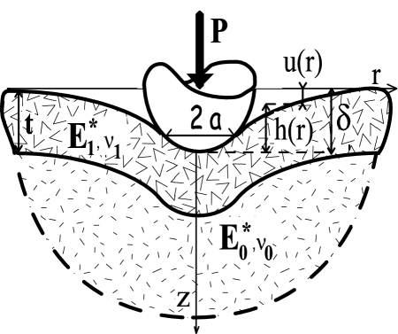
Figure 2:

Figure 3:

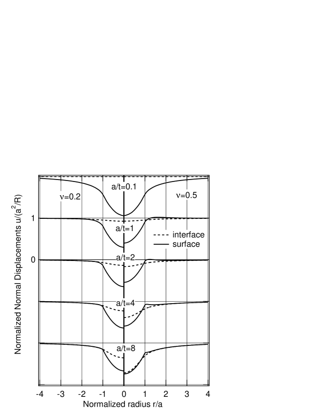
Figure 4:

Figure 5:

Figure 6:

References

- [1] H. J. Gao, C. H. Chiu, and J. Lee. Int. J. Solids Structures, 29, 2471, 1992.
- [2] N. Schwarzer. J. Tribology, 122, 672, 2000.
- [3] E. H. Yoffe. Phil. Mag. Let., 77, 69, 1998.
- [4] H. Y. Yu, S. C. Sanday, and B. B. Rath. J. Mech. Phys. Sol., 38, 745, 1990.
- [5] M. El-Sherbiney and J. Halling. Wear, 40, 325, 1976.
- [6] A. Perriot and E. Barthel. J. Mat. Res., 19, 600, 2004.
- [7] J. Li and T. W. Chou. Int. J. Solids Structures, 34, 4463, 1997.
- [8] R. Podgornik, P. L. Hansen, and V. A. Parsegian. J. Chem. Phys., 119, 1070, 2003.
- [9] I. N. Sneddon. Int. J. Engng. Sci., 3, 47, 1965.
- [10] G. Haiat, M. C. Phan Huy, and E. Barthel. J. Mech. Phys. Sol., 51, 69, 2003.
- [11] J. F. Ganghoffer and A. N. Gent. J. Adh., 48, 75, 1995.
- [12] E. Gacoin, C. Fretigny, A. Chateauminois, A. Perriot, and E. Barthel. to appear in Trib. Let..
- [13] W. C. Oliver and G. M. Pharr. J. Mater. Res., 7, 1564, 1992.