Bose-Einstein condensates in RF-dressed adiabatic potentials

Abstract

Bose-Einstein condensates of ⁸⁷Rb atoms are transferred into radio-frequency (RF) induced adiabatic potentials and the properties of the corresponding dressed states are explored. We report on measurements of the spin composition of dressed condensates. We also show that adiabatic potentials can be used to trap atom gases in novel geometries, including suspending a cigar-shaped cloud above a curved sheet of atoms.

I Introduction

Adiabatic potentials, created using a combination of radio-frequency (RF) and static magnetic fields, are promising tools for confining ultra-cold atoms in novel geometries and for use as beamsplitters in atom interferometry. Examples of proposed trapping geometries include potentials with two dimensional character Zobay01 ; Zobay04 ; Lorent04 , ring shaped potentials Garraway05 , and tunnel arrays Zimmermann06 . The use of adiabatic potentials as a beamsplitter in an atomic interferometry application was recently demonstrated in Schmiedmayer05 . A potential advantage of this technique for exploring atomic superfluids in new geometries over other methods (e.g., optical traps) is that the potential can be very smooth endnote1 .

In this work, we investigate the properties of ultra-cold atoms confined in adiabatic potentials generated through a combination of RF magnetic fields, applied using a small antenna, and static magnetic fields from a Ioffe–Pritchard (IP) magnetic trap. Bose condensed ⁸⁷Rb atoms are created in the $F=1$, $m_{F}=-1$ state in a cigar-shaped axisymmetric IP trap and then transferred into three types of adiabatic potentials: a finite-depth cigar-shaped harmonic trap, a cigar-shaped trap which is strongly anharmonic, and a curved-sheet potential. The primary results presented in this paper are measurements of the population in each $m_{F}$ state for the finite depth and anharmonic potentials and measurements of the displacement of the curved-sheet potential for different frequencies of the RF magnetic field.

II Theory

An atom moving in the presence of static and RF magnetic fields experiences adiabatic potentials as long as there are no Landau-Zener transitions. These adiabatic potentials are provided by a spatially inhomogeneous static magnetic field which gives rise to a spatially varying detuning for the RF magnetic field. In the adiabatic potential, the atom exists in a superposition of hyperfine or Zeeman states, which is a stationary state in the rotating frame. These superposition states are typically referred to as dressed states CohenTannoudji68 .

In our experiment, the dressed states are composed of the $m_{F}=\pm 1$ and $m_{F}=0$ Zeeman states in the $5S_{1/2}$, $F=1$ hyperfine ground state of ⁸⁷Rb. The Zeeman states are coupled by an RF magnetic field $\boldsymbol{B}_{\textrm{rf}}=\cos(\omega t)\boldsymbol{\hat{y}}$, where $\boldsymbol{\hat{z}}$ is the weak direction of the IP trap and the gravitational force acts in the $-\boldsymbol{\hat{y}}$ direction. The frequency $\omega$ of the RF field is tuned near the $m_{F}=0\leftrightarrow m_{F}=+1$ and $m_{F}=0\leftrightarrow m_{F}=-1$ transitions, which are nearly degenerate at the static field magnitudes used here ($<11$ G).

To determine the dressed state wavefunctions, one must solve three coupled Gross-Pitaevskii equations. A simplification of these equations is possible in our system because the interaction strengths between different $m_{F}$ states are nearly equal, and spin exchange rates are small compared to the RF Rabi rate (we estimate spin-exchange rates less than 10 Hz). The many-body wavefunction may therefore be written as $|\psi\rangle=c_{+}|+\rangle\psi_{+}+c_{0}|0\rangle\psi_{0}+c_{-}|-\rangle\psi_{-}$, where $|+\rangle,|0\rangle,|-\rangle$ are the single atom dressed states and $\psi_{+},\psi_{0},\psi_{-}$ are the Thomas–Fermi wavefunctions determined by the corresponding adiabatic potentials. In the dressed-state basis, $|\psi\rangle$ is a stationary state—the numbers of atoms in each dressed state are independent and are determined by the process used to transfer atoms into the adiabatic potentials.

The dressed states can be written in terms of a single angle defined by $\tan\theta=\sqrt{2}\Omega/\delta$,

$$|+\rangle = \frac{1}{2}\left[(1+\cos\theta)|m_{F}=1\rangle+\sqrt{2}\sin\theta|m_{F}=0\rangle\right.$$ (1a)

$$\left.+\frac{\sin^{2}\theta}{1+\cos\theta}|m_{F}=-1\rangle\right],$$

$$|-\rangle = \frac{1}{2}\left[(1-\cos\theta)|m_{F}=1\rangle-\sqrt{2}\sin\theta|m_{F}=0\rangle\right.$$ (1b)

$$\left.+\frac{\sin^{2}\theta}{1-\cos\theta}|m_{F}=-1\rangle\right],$$

$$|0\rangle = \frac{1}{2}\left[-\sqrt{2}\sin\theta|m_{F}=1\rangle+2\cos\theta|m_{F}=0\rangle\right.$$ (1c)

$$\left.+\sqrt{2}\sin\theta|m_{F}=-1\rangle\right].$$

Here, the detuning $\delta=\omega-\omega_{B}$ is measured from the frequency $\omega_{B}=\mu B/\hbar$ of the $|m_{F}=\pm 1\rangle\leftrightarrow|m_{F}=0\rangle$ transitions, which is determined by the local magnetic field $B$ experienced by an atom and the atomic magnetic moment $\mu=g_{F}\mu_{B}$ ($g_{F}=-1/2$ is the $g$-factor for the $F=1$ state, and $\mu_{B}$ is the Bohr magneton). The Rabi rates, $\Omega_{\pm}=-\frac{1}{2}\langle m_{F}=\pm 1|\boldsymbol{\mu}\cdot\boldsymbol{B}_{\textrm{rf}}|m_{F}=0\rangle$, for the $|m_{F}=\pm 1\rangle\leftrightarrow|m_{F}=0\rangle$ transitions depend on the static magnetic field. In our experiment, the rates are nearly equal: $\Omega_{\pm}\approx\Omega\approx 0.483\times\mu_{B}B_{\textrm{rf}}/\hbar$. The dressed state wavefunctions are written in Eq. (1) in a rotating frame defined by $c_{+}=\tilde{c}_{+}e^{i\omega t}$, $c_{-}=\tilde{c}_{-}e^{-i\omega t}$, and $c_{0}=\tilde{c}_{0}$, where the single-atom spin wavefunction is written in the Schrodinger picture as $|\tilde{\psi}\rangle=\tilde{c}_{+}|m_{F}=+1\rangle+\tilde{c}_{-}|m_{F}=0\rangle+\tilde{c}_{-}|m_{F}=-1\rangle$. The dressed states have eigenenergies $E_{+}=\hbar\sqrt{\delta^{2}+2\Omega^{2}}$, $E_{-}=-\hbar\sqrt{\delta^{2}+2\Omega^{2}}$, and $E_{0}=0$.

The shape of the adiabatic potentials is determined by the effect of the inhomogeneous magnetic field created by the IP trap, where

$$B(\boldsymbol{r})^{2}\approx B_{0}^{2}+(C_{1}^{2}-B_{0}B_{2})r^{2}+2B_{0}B_{2}z^{2},$$ (2)

near the center of the trap Metcalf87 . Here, $B_{0}$ is the bias field, i.e., the magnitude of the field at the center of trap, $C_{1}$ is the radial gradient, and $B_{2}$ is the axial curvature. For the work presented in this paper, $B_{0}=1.33(1)\textrm{ MHz}\times h/\mu$, and $C_{1}=355(2)$ G/cm and $B_{2}=129(2)\textrm{ G/cm}^{2}$ (determined from measurements of the harmonic trapping frequencies). The adiabatic potentials for the $|+\rangle$ and $|-\rangle$ states are $U_{\pm}=\pm\sqrt{[\mu B(\boldsymbol{r})]^{2}+2(\hbar\Omega)^{2}}+mgy$, where $g$ is the local acceleration due to gravity. The $|0\rangle$ state is only affected by gravity and experiences a potential $U_{0}=mgy$. The adiabatic potentials are shown in Fig. 1.

The shape of the adiabatic potentials depends on the detuning, $\Delta=\omega-\omega_{0}$, relative to the resonance at the trap center, $\omega_{0}=\mu B_{0}/\hbar$. We summarize here the shape of the adiabatic potentials, starting with the $U_{-}$ potential. The $U_{-}$, $\Delta>0$ potential is the familiar potential utilized for forced RF-induced evaporative cooling evapcooling . This potential is harmonic near the central minimum and the curvature there is independent of detuning, except for small (compared with the Rabi rate) detunings. The $U_{-}$, $\Delta<0$ potential is not confining.

In contrast to the $U_{-}$ potential, the $U_{+}$ potential is always confining with a trapping geometry that depends strongly on detuning: for large and negative $\Delta$, it is harmonic near the potential minimum. For small and negative $\Delta$, the $U_{+}$ potential is quartic in the absence of gravity; gravitational sag results in an overall trapping potential for this case which is strongly anharmonic and cannot be characterized as purely quartic. For $\Delta>0$, the $U_{+}$ potential is an ellipsoidal shell in the absence of gravity. Atoms in the $|+\rangle$ state are forced by gravity to occupy a curved sheet in the bottom of this shell.

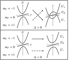
Figure 1: Adiabatic potentials for the $F=1$ state in the presence of gravity. The potential $U$ is shown along the $\boldsymbol{\hat{y}}$ direction for the $|+\rangle$, $|0\rangle$, and $|-\rangle$ states on the right and with no RF magnetic field present on the left. The arrows indicate how the $m_{F}$ states transform when the RF field is turned on adiabatically for positive ($\Delta>0$) and negative ($\Delta<0$) detuning.

III Experiments

The dressed states are primarily characterized by the population in each $m_{F}$ state. We investigate the $m_{F}$ state composition of the dressed states in the $U_{-}$ and $U_{+}$ potentials for $\Delta>0$ and $\Delta<0$, respectively, by measuring the population in the $m_{F}=0$ and $m_{F}=-1$ states after the RF is turned off suddenly. We also show that measuring the populations in the $m_{F}$ basis for different detunings is a sensitive method for determining the Rabi rate.

We begin by creating a condensate of approximately $5\times 10^{5}$ ⁸⁷Rb atoms in the $F=1$, $m_{F}=-1$ state with no observable thermal component via RF evaporative cooling (we use an apparatus similar to that described in Lewandowski03 ). The atoms are trapped in a Ioffe–Pritchard type magnetic trap as described above with radial and axial trapping frequencies $\omega_{r}=231(8)$ Hz, and $\omega_{z}=14.5(3)$ Hz, respectively. Atoms are imaged via a standard absorption imaging technique, using light resonant with the $5S_{1/2},F=2$ to $5P_{3/2},F=3$ cycling transition. Immediately before the probe beam is switched on, atoms are optically pumped from the $F=1$ manifold to the $F=2$ manifold using light tuned to the $5S_{1/2},F=1$ to $5P_{3/2},F=2$ transition. RF signals are coupled to the atoms by an antenna which is a three turn, 10 mm radius coil located 1.5 cm from the atoms in the $\boldsymbol{\hat{y}}$ direction.

To measure the $m_{F}$ state composition, the RF field is turned on slowly to transfer all the atoms in the condensate from the $m_{F}=-1$ state to a single dressed state, and then turned off suddenly to project the dressed state on to the $m_{F}$ basis. Once a condensate is created, the RF power is increased linearly from 0 to 35 dBm (of which a fraction is coupled into the RF antenna) over 5 ms at 1.10 MHz (1.75 MHz) for data taken with $\Delta<0$ ($\Delta>0$). The RF frequency is swept linearly at 10 kHz/ms to the value at which we wish to measure the spin composition; the RF is then shut off suddenly (the RF source is turned off within 3 ns). Turning off the RF much faster than the effective Rabi rate projects the dressed states into the $m_{F}$ basis, making it possible to investigate the spin composition by measuring the relative number of atoms in each $m_{F}$ state. After waiting 3 ms for the $m_{F}=0$ atoms to fall and spatially separate from the $m_{F}=-1$ atoms, the magnetic trap is shut off. This 3 ms delay also forces any $m_{F}=+1$ atoms to be ejected from the trapping region by the inhomogeneous magnetic field from the IP trap. The $m_{F}=0$ and $m_{F}=-1$ clouds are imaged 7 ms after the magnetic trap is turned off. We verify that the frequency sweep is adiabatic by sweeping the RF source back to the initial frequency (1.10 MHz or 1.75 MHz) before turning off the RF field and observing no loss of atoms.

The number of atoms in each $m_{F}$ state is obtained by fitting the absorption images to the Thomas–Fermi profile expected for a BEC. The data in Fig. 2 show the experimentally determined ratio of $m_{F}=0$ atoms to the total number of $m_{F}=0$ and $m_{F}=-1$ atoms for different final RF frequencies; as many as 20% of the atoms are observed in the $m_{F}=0$ state. The data in Fig. 2 are fitted to

$$\frac{N_{0}}{N_{0}+N_{-1}}=\frac{4\Omega^{2}}{4\Omega^{2}+(|\delta|+\sqrt{\delta^{2}+2\Omega^{2}})^{2}},$$ (3)

which is the relative Zeeman state distribution expected from Eq. (1) endnote3 . Only points at detunings beyond $\pm 50$ kHz, where gravitational sag is calculated to shift the measured ratio by less than 1%, are included in the fit. The Rabi rate and $\omega_{0}$ are left as free parameters in the fit; the values obtained are $\Omega=2\pi\times 24.6(5)$ kHz and $\omega_{0}=2\pi\times 1.328(2)$ MHz, corresponding to an RF field strength $B_{\textrm{rf}}=36.3(7)$ mG. Determining the Rabi rate is normally very difficult in cold-atom experiments involving transitions between magnetically trapped and untrapped states, because Rabi oscillations cannot be directly observed and uncertainty in the geometry of the RF antenna. We are able to determine $\Omega$ to within 2% via spin composition measurements. The response of the RF source and antenna do not vary significantly over the frequency range covered by the data in Fig. 2.

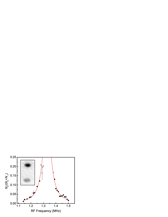
Figure 2: Ratio of $m_{F}=0$ atoms to total number of $m_{F}=0$ and $m_{F}=-1$ atoms versus RF frequency. Data for RF frequencies greater (less) than 1.328 MHz represent atoms confined in the $U_{-}$ ($U_{+}$) potential. Each data point represents a single image, except the points with error bars, which are each an average of 7 measurements; the error bars indicate the standard deviation of these measurements. The solid red line is a fit to Eq. (3). Open circles represent data points for which gravitational sag is calculated to shift the measured ratio by more than 1% and are not included in the fit. The inset shows a typical image used to obtain the data; the field of view is approximately 260 $\mu$m by 370 $\mu$m. The lower (upper) cloud consists of $m_{F}=0$ ($m_{F}=-1$) atoms.

The simplest example of using adiabatic potentials to confine ultra-cold atoms in a novel geometry can be realized using the $|+\rangle$ state for positive detuning. Atoms in the $U_{+}$ potential for $\Delta>0$ occupy a curved sheet, which is the bottom part of an ellipsoidal shell potential Zobay01 . We characterized the shape of the $U_{+}$ potential by measuring the displacement of atoms in the $|+\rangle$ state from the minimum of the $m_{F}=-1$ potential (in the absence of the RF field).

Atoms are transferred into the $U_{+}$ potential by turning on the RF field at $\Delta<0$ and sweeping the frequency through $\omega_{0}$ to the value where the displacement will be measured. Zobay01 ; Lorent04 . In general, care must be taken to sweep slowly enough to adiabatically transfer a BEC into the $U_{+}$ potential. We made no attempt to sweep adiabatically because the measured displacement was found to be independent of the details of the frequency sweep. For the data shown in Fig. 3, the RF is turned on at 1.10 MHz and swept at 31 kHz/ms using $\Omega\approx 2\pi\times 40$ kHz. After transferring atoms into the $U_{+}$ potential, the atoms are held for 4 ms and then imaged in the trap. The center of the atom cloud is determined by a Gaussian fit to the absorption image. Fig. 3 shows the measured displacement from the the minimum of the $m_{F}=-1$ potential for different RF frequencies. The error bars account for uncertainty in the magnification of our imaging system.

The measured data agree well with the displacement expected for an IP magnetic trap. The solid red line in Fig. 3 is the displacement calculated using the magnetic field minimum in Eq. (2) at $z=0$. We have ignored gravitational sag, calculated to be less than 1 $\mu$m for detunings beyond 0.2 MHz. At large detunings, the displacement is dominated by the radial gradient of the IP trap. For small detunings, the cloud samples only the field near the center of the IP potential, and the displacement is quadratic in detuning. Plotting Fig. 3 as RF frequency vs. displacement produces a map of the radial field of the IP trap. This provides a method to measure the radial field to high accuracy—fitting the data in Fig. 3 to the equation used to calculate the solid red line, but leaving $\omega_{0}$ and $C_{1}$ as free parameters, yields $C_{1}=357(2)$ G/cm. The radial gradient obtained using this technique is in excellent agreement with the value derived from measuring the IP trap frequencies through “sloshing” motion of the condensate.

We have also realized an unusual trapping geometry in which a cigar-shaped cloud of atoms is trapped above a curved sheet of atoms. By increasing the frequency sweep rate and/or decreasing the RF power, it is possible to transfer only a fraction of the atoms to the $U_{+}$ potential. Under these conditions, Landau-Zener transitions result in atoms trapped in both the $U_{+}$ and $U_{-}$ potentials, as seen in the inset to Fig. 3. Here, the detuning was $\Delta=2\pi\times 1$ MHz, and the loading ramp was altered so that the frequency sweep rate was 300 kHz/ms and $\Omega=2\pi\times 3.3$ kHz within $\pm 40\textrm{ kHz}\times 2\pi$ of $\omega_{0}$.

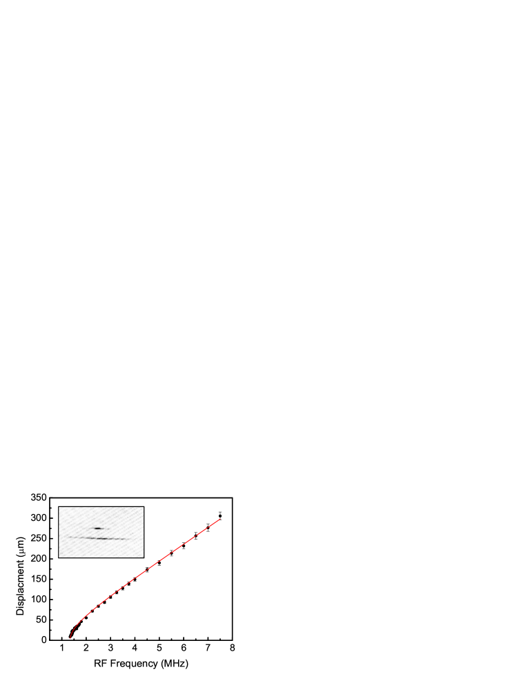
Figure 3: Displacement from the IP trap center for atoms trapped in $U_{+}$ potential for different RF frequencies. The solid red line shows the calculated displacement. The inset shows atoms simultaneously loaded into the $U_{-}$ (upper cloud) and $U_{+}$ potentials at $\Delta=2\pi\times 1$ MHz. The field of view for the inset (taken while the atoms were trapped) is approximately 640 $\mu$m by 390 $\mu$m.

We briefly discuss the prospects for obtaining a 2D BEC in the $U_{+}$, $\Delta>0$ potential. Motion around the bottom of this potential is characterized by three different harmonic oscillator frequencies: a large radial frequency and two small frequencies along directions which experience pendulum-like motion Zobay04 ; Lorent04 . For the $U_{+}$ potential at $\Delta=2\pi\times 1$ MHz and $\Omega=2\pi\times 40$ kHz, the radial and two pendular frequencies are calculated to be 900 Hz and 60 Hz and 4 Hz, respectively. These frequencies are calculated using a classical normal-modes calculation and the magnetic field from Eq. (2). We observed a lifetime of 4(2) s and a heating rate of 4.5(3) $\mu$K/s under these conditions. Sources of atom loss may be Landau–Zener transitions to untrapped states Zobay04 ; three body recombination may also play a role because the non-adiabatic loading into this potential can transiently increase the density endnote2 . Because adiabatic transfer into the the 2D regime is quite slow, due to the low pendular trap frequencies of the $U_{+}$ potential, we expect obtaining a condensate in the 2D regime to be difficult without significant improvement to the heating rate. A large heating rate was also observed in Lorent04 , where it was attributed to noise in the RF frequency. Finally, we remark that we have observed partially condensed clouds upon release from the $U_{+}$ potential for $\Delta$ up to 1.5 MHz after rapid (non-adiabatic) loading (31 kHz/ms frequency sweep rate), indicating that the condensate is not destroyed immediately by the loading process.

IV Conclusion

In conclusion, we have investigated the nature of RF dressed potentials for magnetically trapped ⁸⁷Rb in the $F=1$ state and measured the $m_{F}$ state composition of the dressed states. We have also studied the shape of the ellipsoidal $U_{+}$ potential. Potentially useful techniques for measuring the RF Rabi rate and for directly characterizing the radial field of a magnetic trap were also demonstrated.

Future directions for this research include creating ring traps Garraway05 ; Schmiedmayer06 , which are promising for use as atomic Sagnac interferometers. Courteille et. al. Zimmermann06 also recently proposed a scheme to create versatile potentials using multiple RF frequencies. An important future step is to characterize and address heating and loss mechanisms in dressed state potentials. Because the dressed states are superpositions of the atomic spin states, a related question of particular interest concerns the nature of spin exchange collisions for dressed states.

We acknowledge funding from the Office of Naval Research (Grant No. N000140410490), the National Science Foundation (Award No. 0448354), the Sloan Foundation, and the University of Illinois Research Board. We thank Deborah Jin for a careful reading of this manuscript.

References

- (1) O. Zobay and B.M. Garraway, Phys. Rev. Lett. 86, 1195 (2001).
- (2) O. Zobay and B.M. Garraway, Phys. Rev. A 69, 023605 (2004).
- (3) Y. Colombe et al., Europhys. Lett. 67, 593 (2004); Y. Colombe et al., J. Phys. IV France 116, 247 (2004).
- (4) O. Morizot et al., physics/0512015.
- (5) Ph. W. Courteille et al., J. Phys. B 39, 1055 (2006).
- (6) T. Schumm et al., Nature Phys. 1, 57 (2005).
- (7) The combined RF-frequency and static magnetic potential is smooth provided that the trapping region is much smaller than the characteristic dimensions of the magnetic trap.
- (8) C. Cohen-Tannoudji, B. Diu and F. Laloë, Quantum Mechanics (Wiley, New York, 1968)
- (9) T. Bergeman et al., Phys. Rev. A 35, 1535 (1987)
- (10) W. Petrich et al., International Conference on Atomic Physics XIV, 1994, p. 1M-7; K.B. Davis et al., ibid., p. 1M-3.
- (11) H. J. Lewandowski et al., J. Low Temp. Phys. 132, 309 (2003)
- (12) We plot the ratio because we cannot measure the number of atoms in the state, and hence we cannot determine the total number of atoms.
- (13) Based on the calculated trap frequencies, the equilibrium density is expected to be lower in the adiabatic potential than in the IP trap.
- (14) I. Lesanovsky et al., physics/0510076.