Surface plasmon in metallic nanoparticles: renormalization effects due to electron-hole excitations

Abstract

The electronic environment causes decoherence and dissipation of the collective surface plasmon excitation in metallic nanoparticles. We show that the coupling to the electronic environment influences the width and the position of the surface plasmon resonance. A redshift with respect to the classical Mie frequency appears in addition to the one caused by the spill-out of the electronic density outside the nanoparticle. We characterize the spill-out effect by means of a semiclassical expansion and obtain its dependence on temperature and the size of the nanoparticle. We demonstrate that both, the spill-out and the environment-induced shift are necessary to explain the experimentally observed frequencies and confirm our findings by time-dependent local density approximation calculations of the resonance frequency. The size and temperature dependence of the environmental influence results in a qualitative agreement with pump-probe spectroscopic measurements of the differential light transmission.

I Introduction

One of the most prominent features of a metallic nanoparticle subject to an external driving field is a collective electronic excitation, the so-called surface plasmon. deheer ; brack ; kreibig_vollmer Since the first spectroscopic measurement of the related resonance in the absorption cross section of free sodium clusters, deheer87 much progress has been made in the characterization of this collective resonance, both experimentally deheer ; brechignac92 ; haberland ; brechignac ; reiners_cpl ; reiners and theoretically. brack ; ekardt ; barma ; yannouleas ; bertsch ; madjet The proposed application of metallic nanoparticles boyer or nanocrystals dahan as markers in biological systems such as cells or neurons renders crucial the understanding of their optical properties.

The first experiments have been made on ensembles of nanoparticles, where the inhomogeneous broadening of the resonance resulting from the size dependence of the resonance frequency masks the homogeneous linewidth. lamprecht ; stietz ; bosbach In order to gain detailed information on the collective resonance, considerable effort has lately been devoted to the measurement of single-cluster optical properties. klar ; sonnichsen ; arbouet ; dijk ; berciaud The possibility of overcoming the inhomogeneous broadening resulted in a renewed interest in the theory of the optical response of metallic clusters.

From a fundamental point of view, surface plasmons appear as interesting resonances to study given the various languages that we can use for their description, which are associated with different physical images. At the classical level, a nanoparticle can be considered as a metallic sphere of radius $a$ described by a Drude dielectric function $\epsilon(\omega)=1-\omega_{\rm p}^{2}/\omega(\omega+{\rm i}\gamma_{\rm i})$, where $\omega_{\rm p}=\sqrt{4\pi n_{\rm e}e^{2}/m_{\rm e}}$ is the plasma frequency, $\gamma_{\rm i}^{-1}$ the relaxation or collision time, while $e$, $m_{\rm e}$ and $n_{\rm e}$ stand for the electron charge, mass and bulk density, respectively. Classical electromagnetic theory for a sphere in vacuum yields a resonance at the Mie frequency $\omega_{\rm M}=\omega_{\rm p}/\sqrt{3}$. deheer ; brack ; kreibig_vollmer

At the quantum level, linear response theory for an electron gas confined by a positive jellium background yields a resonance at the Mie frequency $\omega_{\rm M}$ with a total linewidth kubo

$$\gamma_{\rm t}(a)=\gamma_{\rm i}+\gamma(a).$$ (1)

Thus, in addition to the intrinsic linewidth $\gamma_{\rm i}$, we have to consider a size-dependent contribution which can be expressed as kubo ; barma ; yannouleas

$$\gamma(a)=\frac{3v_{\rm F}}{4a}g_{0}\left(\frac{\varepsilon_{\rm F}}{\hbar\omega_{\rm M}}\right)$$ (2)

where $\varepsilon_{\rm F}=\hbar^{2}k_{\rm F}^{2}/2m_{\rm e}$ and $v_{\rm F}$ are the Fermi energy and velocity, respectively, and $g_{0}$ is a smooth function that will be given in (36). yannouleas_85 The size-dependent linewidth $\gamma(a)$ results from the decay of the surface plasmon into particle-hole pairs by a Landau damping mechanism, which is the dominant decay channel for nanoparticle sizes $0.5\,\mathrm{nm}\lesssim a\lesssim 5\,\mathrm{nm}$ considered in this work. For larger clusters, the interaction of the surface plasmon with the external electromagnetic field becomes the preponderant source of damping. kreibig_vollmer

In a quantum many-body approach, the surface plasmon appears as a collective excitation of the electron system. Discrete-matrix random phase approximation (RPA) provides a useful representation since the eigenstates of the correlated electron system are expressed as superpositions of particle-hole states built from the Hartree-Fock ground state. Following similar approaches developed for the study of giant resonances in nuclei, Yannouleas and Broglia yannouleas proposed a partition of the many-body RPA Hilbert space into a low-energy sector (the restricted subspace), containing particle-hole excitations with low energy, and a high-energy sector (the additional subspace). The surface plasmon arises from a coherent superposition of a large number of basis states of the restricted subspace. Its energy lies in the high-energy sector, and therefore the mixture with particle-hole states of the additional subspace results in the broadening of the collective resonance.

An alternative to the previous approaches is given by numerical calculations using the time-dependent local density approximation (TDLDA) within a jellium model. ekardt ; bertsch_RPA The absorption cross section

$$\sigma(\omega)=\frac{4\pi e^{2}\omega}{3c}\sum_{f}\left|\langle f|z|0\rangle\right|^{2}\delta(\hbar\omega-E_{f}+E_{0})$$ (3)

can be obtained from the dipole matrix elements between the ground state $|0\rangle$ and the excited states $|f\rangle$ of the electron system with energies $E_{0}$ and $E_{f}$, respectively. $c$ is the speed of light. In the absorption cross section, the surface plasmon appears as a broad resonance (see Fig. 1) centered at a frequency $\omega_{\rm sp}$ close to $\omega_{\rm M}$ and with a linewidth approximately described by (1).

Figure 1: Absorption cross section $\sigma(\omega)$ in arbitrary units extracted from TDLDA calculations for a sodium cluster containing $N=832$ valence electrons. The classical Mie frequency is $\omega_{\rm M}$, while $\tilde{\omega}_{\rm M}$ is the frequency of the surface plasmon resonance taking into account the spill-out effect. It has been obtained with the Kohn-Sham self-consistent ground-state density as explained in Sec. IV.3. $\omega_{\rm sp}$ corresponds to the position of the maximum of the absorption curve.

Finally, the separation in center-of-mass and relative coordinates for the electron system gerchikov ; weick within a mean-field approach allows to describe the surface plasmon as the oscillation of a collective coordinate, which is damped by the interaction with an environment constituted by a large number of electronic degrees of freedom. Within such a decomposition, the effects of finite size, a dielectric material, weick or the finite temperature of the electron gas are readily incorporated. Since the excitation by a laser field in the optical range only couples to the electronic center of mass, this approach is particularly useful.

The experimentally observed resonance frequencies are smaller than the Mie frequency $\omega_{\rm M}$, deheer ; brechignac92 ; reiners and this is qualitatively captured by TDLDA calculations since $\omega_{\rm sp}<\omega_{\rm M}$ (see Fig. 1). This redshift is usually attributed to the so-called spill-out effect. brack The origin of this quantum effect is a nonzero probability to find electrons outside the nanoparticle, which results in a reduction of the effective frequency for the center-of-mass coordinate. If a fraction $N_{\rm out}/N$ of the electrons is outside the geometrical boundaries of the nanoparticle, we can expect that the electron density within the nanoparticle is reduced accordingly and the frequency of the surface plasmon is given by

$$\tilde{\omega}_{\rm M}=\omega_{\rm M}\sqrt{1-\frac{N_{\rm out}}{N}}.$$ (4)

We will see in Sec. II that such an estimation can be formalized considering the form of the confining potential. It has been known for a long time brack that $\tilde{\omega}_{\rm M}>\omega_{\rm sp}$, and therefore the spill-out effect is not sufficient to explain the redshift of the surface plasmon frequency as it can be seen in Fig. 1. Recently, the coupling to the electronic environment has been invoked as an additional source of frequency shift. gerchikov ; hagino In this work we provide an estimation of such a contribution (analogous to the Lamb shift of atomic physics cohen ) and its parametric dependence on the particle size and electron temperature (see Sec. V). In our approach, we always adopt a spherical jellium model for the ionic background which is expected to yield reliable results for not too small nanoparticle sizes. Despite the fact that we have to make several approximations, we find that this additional shift implies a reduction of the surface plasmon frequency, in qualitative agreement with the TDLDA calculations. However it is known brack that the experimental resonance frequency is even lower than the TDLDA prediction. This could be due to the ionic degrees of freedom.

In femtosecond time-resolved pump-probe experiments on metallic nanoparticles bigot ; delfatti the surface plasmon plays a key role. The pump field heats the electron system via an excitation of the collective mode. The probe then tests the absorption spectrum of the hot electron gas in the nanoparticle, and therefore it is important to understand the temperature dependences of the surface plasmon linewidth and of the frequency of the resonance.

The paper is organized as follows: In Sec. II, we present our model and the separation of the electronic degrees of freedom into the center of mass and the relative coordinates. The center-of-mass coordinate provides a natural description of the spatial collective oscillations of the electronic cloud around its equilibrium position resulting from a laser excitation. Its coupling to the relative coordinates, described within the mean-field approximation, is responsible for the broadening of the surface plasmon resonance that we evaluate in Sec. III. We determine the dependence of the surface plasmon linewidth on the size of the nanoparticle and explore its low-temperature properties. In Sec. IV, we evaluate the spill-out effect, focusing on its dependence on size and temperature of the nanoparticle. We show by means of TDLDA calculations that the spill-out effect is not sufficient to describe the redshift of the surface plasmon frequency as compared to its classical value. In Sec. V, we propose an estimation of the environment-induced redshift of the surface plasmon resonance which adds to the spill-out effect. Both effects together, spill-out and frequency shift due to the electronic environment, could explain the observed redshift of the resonance frequency. In Sec. VI, we draw the consequences of our findings for pump-probe experiments. The temperature dependences of the linewidth and frequency of the surface plasmon resonance peak permit to qualitatively explain the time dependence of the measured optical transmission as a function of the delay between the pump and the probe laser field. We finally conclude and draw the perspectives of this work in Sec. VII.

II Coupling of the surface plasmon to electron-hole excitations

Treating the ionic background of the nanoparticle as a jellium sphere of radius $a$ with sharp boundaries, the Hamiltonian for the valence electrons is given by

$$H=\sum_{i=1}^{N}\left[\frac{p_{i}^{2}}{2m_{\rm e}}+U(r_{i})\right]+\frac{e^{2}}{2}\sum_{\begin{subarray}{c}i,j=1\\ (i\neq j)\end{subarray}}^{N}\frac{1}{\left|{\bf r}_{i}-{\bf r}_{j}\right|},$$ (5)

where ${\bf r}_{i}$ is the position of the $i^{\rm th}$ particle and $r_{i}=|{\bf r}_{i}|$. The single-particle confining potential

$$U(r)=\frac{Ne^{2}}{2a^{3}}\left(r^{2}-3a^{2}\right)\Theta(a-r)-\frac{Ne^{2}}{r}\Theta(r-a)$$ (6)

is harmonic with frequency $\omega_{\rm M}=\sqrt{Ne^{2}/m_{\rm e}a^{3}}$ inside the nanoparticle and Coulomb-like outside. $\Theta(x)$ denotes the Heaviside step function. In principle, the photoabsorption cross section (3) can be determined from the knowledge of the eigenstates of $H$. However, except for clusters containing only few atoms, this procedure is exceedingly difficult, and one has to treat this problem using suitable approximation schemes.

II.1 Separation into collective and relative coordinates

A particularly useful decomposition gerchikov of the Hamiltonian (5) can be achieved by introducing the coordinate of the electronic center of mass ${\bf R}=\sum_{i}{\bf r}_{i}/N$ and its conjugated momentum ${\bf P}=\sum_{i}{\bf p}_{i}$. The relative coordinates are denoted by ${\bf r}_{i}^{\prime}={\bf r}_{i}-{\bf R}$ and ${\bf p}_{i}^{\prime}={\bf p}_{i}-{\bf P}/N$. Then, the Hamiltonian (5) can be written as

$$H=\frac{{\bf P}^{2}}{2Nm_{\rm e}}+H_{\rm rel}+\sum_{i=1}^{N}\left[U(|{\bf r}_{i}^{\prime}+{\bf R}|)-U(r_{i}^{\prime})\right],$$ (7)

where

$$H_{\rm rel}=\sum_{i=1}^{N}\left[\frac{{p_{i}^{\prime}}^{2}}{2m_{\rm e}}+U(r_{i}^{\prime})\right]+\frac{e^{2}}{2}\sum_{\begin{subarray}{c}i,j=1\\ (i\neq j)\end{subarray}}^{N}\frac{1}{\left|{\bf r}_{i}^{\prime}-{\bf r}_{j}^{\prime}\right|}$$ (8)

is the Hamiltonian for the relative-coordinate system.

Assuming that the displacement $\bf R$ of the center of mass is small compared to the size of the nanoparticle, we can expand the last term on the r.h.s. of (7). To second order, we obtain

$$U(|{\bf r}^{\prime}+{\bf R}|)-U(r^{\prime})\simeq{\bf R}\cdot\bm{\nabla}U(r^{\prime})+\frac{1}{2}\left({\bf R}\cdot\bm{\nabla}\right)^{2}U(r^{\prime}),$$ (9)

where the derivatives are taken at ${\bf r}={\bf r}^{\prime}$ (${\bf R}={\bf 0}$). Choosing the oscillation axis of the center of mass in the $z$-direction, ${\bf R}=Z{\bf e}_{z}$, we obtain with (6)

$${\bf R}\cdot\bm{\nabla}U(r^{\prime})=Zm_{\rm e}\omega_{\rm M}^{2}\left[z^{\prime}\Theta(a-r^{\prime})+\frac{z^{\prime}a^{3}}{{r^{\prime}}^{3}}\Theta(r^{\prime}-a)\right]$$ (10)

and

$$\left({\bf R}\cdot\bm{\nabla}\right)^{2}U(r^{\prime}) =$$ (11)

$$Z^{2}Ne^{2} \left[\frac{1}{a^{3}}\Theta(a-r^{\prime})+\frac{1-3\cos^{2}{\theta^{\prime}}}{{r^{\prime}}^{3}}\Theta(r^{\prime}-a)\right].$$

Eq. 10 represents a linear coupling in $Z$ between the center-of-mass and the relative-coordinate system. In second order, the first term on the r.h.s. of (11) is the dominant contribution to the confinement of the center of mass. The second term on the r.h.s. of (11) is of second order in the coupling and therefore is neglected compared to the first-order coupling of (10).

Inserting (9) and (11) into (7), we obtain

$$H=\frac{{\bf P}^{2}}{2Nm_{\rm e}}+\frac{1}{2}\frac{Ne^{2}}{a^{3}}{\bf R}^{2}\sum_{i=1}^{N}\Theta(a-r_{i})+H_{\rm rel}+H_{\rm c},$$ (12)

where

$$H_{\rm c}=\sum_{i=1}^{N}{\bf R}\cdot\left[\bm{\nabla}U(r_{i}^{\prime})\right]\Big{|}_{{\bf R}={\bf 0}}$$ (13)

is the coupling between the center-of-mass and the relative coordinates to first order in the displacement $\bf R$ of the center of mass according to (10). The remaining sum over $i$ in (12) yields the number of electrons inside the nanoparticle, i.e., $N-N_{\rm out}$ where $N_{\rm out}$ is the number of spill-out electrons, and finally we rewrite the Hamiltonian as

$$H=H_{\rm cm}+H_{\rm rel}+H_{\rm c}.$$ (14)

The Hamiltonian of the center-of-mass system is

$$H_{\rm cm}=\frac{{\bf P}^{2}}{2Nm_{\rm e}}+\frac{1}{2}Nm_{\rm e}{\tilde{\omega}_{\rm M}}^{2}{\bf R}^{2}.$$ (15)

It is the Coulomb tail of the single-particle confinement (6) which yields the frequency $\tilde{\omega}_{\rm M}$ given in (4) instead of $\omega_{\rm M}$ for the effective harmonic trap that is experienced by the center-of-mass system.

Eq. 14 with (8), (13), and (15) recovers up to the second order in $\bf R$ the decomposition derived in Ref. gerchikov, . However, in contrast to that work, we do not need to appeal to an effective potential for the center-of-mass system.

The structure of (14) is typical for quantum dissipative systems: weiss The system under study ($H_{\rm cm}$) is coupled via $H_{\rm c}$ to an environment or “heat bath” $H_{\rm rel}$, resulting in dissipation and decoherence of the collective excitation. In our case the environment is peculiar in the sense that it is not external to the nanoparticle, but it represents a finite number of degrees of freedom of the gas of conduction electrons. If the single-particle confining potential $U$ of (6) were harmonic for all $r$, Kohn’s theorem kohn would imply that the center of mass and the relative coordinates are decoupled, i.e., $H_{\rm c}=0$. Thus, for a harmonic potential $U$ the surface plasmon has an infinite lifetime. The Coulomb part of $U$ in (6) leads to the coupling of the center of mass and the relative coordinates, and translates into the decay of the surface plasmon. Furthermore, it reduces the frequency of the center-of-mass system from $\omega_{\rm M}$ according to (4).

II.2 Mean-field approximation

Introducing the usual annihilation operator

$$b=\sqrt{\frac{Nm_{\rm e}\tilde{\omega}_{\rm M}}{2\hbar}}Z+\frac{\rm i}{\sqrt{2Nm_{\rm e}\hbar\tilde{\omega}_{\rm M}}}P_{Z}$$ (16)

where $P_{Z}$ is the momentum conjugated to $Z$, and the corresponding creation operator $b^{\dagger}$, $H_{\rm cm}$ reads

$$H_{\rm cm}=\hbar\tilde{\omega}_{\rm M}b^{\dagger}b.$$ (17)

Since the electron-electron interaction appears in the Hamiltonian (8), it is useful to describe $H_{\rm rel}$ within a mean-field approximation. One can write

$$H_{\rm rel}=\sum_{\alpha}\varepsilon_{\alpha}c_{\alpha}^{\dagger}c_{\alpha},$$ (18)

where $\varepsilon_{\alpha}$ are the eigenenergies in the effective mean-field potential $V$ and $c_{\alpha}^{\dagger}$ ($c_{\alpha}$) are the creation (annihilation) operators associated with the corresponding one-body eigenstates $|\alpha\rangle$. The mean-field potential $V$ can be determined with the help of Kohn-Sham LDA numerical calculations. In Fig. 2, we show it as a function of $r/a_{0}$ where $a_{0}\simeq 0.53\,\mathrm{\AA}$ is the Bohr radius, for a nanoparticle containing $N=1760$ valence electrons. We see that it is relatively flat at the interior of the nanoparticle, and presents a steep increase at the boundary. The potential jump is often approximated by a true discontinuity at $r=a$. However, the details of the self-consistent potential close to the surface may be crucial for some properties, as we show in Sec. IV.3.

Figure 2: LDA self-consistent potential $V$ as a function of the radial coordinate $r$ for a sodium nanoparticle containing $N=1760$ valence electrons. The radius $a$ is indicated by the vertical dotted line. The Fermi level is marked by the dashed line.

Inserting (10) into the coupling Hamiltonian $H_{\rm c}$ (13), and expressing the $Z$-coordinate in terms of the creation and annihilation operators of (16), one obtains in second quantization

$$H_{\rm c}=\Lambda\left(b^{\dagger}+b\right)\sum_{\alpha\beta}d_{\alpha\beta}c_{\alpha}^{\dagger}c_{\beta},$$ (19)

where

$$d_{\alpha\beta}=\langle\alpha|\left[z\Theta(a-r)+\frac{za^{3}}{r^{3}}\Theta(r-a)\right]|\beta\rangle$$ (20)

is the matrix element between two eigenstates of the unperturbed mean-field problem. In (19), we have defined the constant $\Lambda=\sqrt{\hbar m_{\rm e}\omega_{\rm M}^{3}/2N}$ and neglected the spill-out for the calculation of the coupling when we expressed $Z$ in terms of $b$ and $b^{\dagger}$. The sums over $\alpha$ and $\beta$ in (19) are restricted to the additional (high energy) RPA subspace mentioned in the introduction. If initially the center of mass is in its first excited state, the coupling $H_{\rm c}$ allows for the decay of the collective excitation into particle-hole pairs in the electronic environment $H_{\rm rel}$, the so-called Landau damping. bertsch ; weick ; molina

III Temperature dependence of the surface plasmon linewidth

In this section, we address a semiclassical calculation of the surface plasmon linewidth and extend our zero-temperature results of Ref. weick, to the case of finite temperatures. We are interested in nanoparticles with a large number of confined electrons, typically of the order of $10^{2}$ to $10^{4}$. Thus, the Fermi energy is much larger than the mean one-body level spacing and the semiclassical approximation can be applied.

III.1 Fermi’s golden rule

When the displacement of the center of mass is much smaller than the size of the nanoparticle, it is possible to linearize the coupling Hamiltonian as it was done in Sec. II. The weak coupling regime allows to treat $H_{\rm c}$ as a perturbation to the uncoupled Hamiltonian $H_{\rm cm}+H_{\rm rel}$. Assuming that initially the center of mass is in its first excited state $|1_{\rm cm}\rangle$, i.e., a surface plasmon is excited, two processes limit the surface plasmon lifetime: the decay into the ground state with creation of a particle-hole pair and the excitation to the second state of the center of mass accompanied by the annihilation of a particle-hole pair. Obviously, this last process is only possible at finite temperatures. Then, Fermi’s golden rule yields the linewidth

$$\gamma=\frac{2\pi}{\hbar}\sum_{\begin{subarray}{c}F_{\rm cm}\\ I_{\rm rel},F_{\rm rel}\end{subarray}} P_{I_{\rm rel}}\left|\langle F_{\rm cm},F_{\rm rel}|H_{\rm c}|1_{\rm cm},I_{\rm rel}\rangle\right|^{2}$$

$$\times\delta(\hbar\tilde{\omega}_{\rm M}-\varepsilon_{F_{\rm cm}}+\varepsilon_{I_{\rm rel}}-\varepsilon_{F_{\rm rel}})$$ (21)

for the collective state $|1_{\rm cm}\rangle$. In the golden rule, $|F_{\rm cm}\rangle$ and $|F_{\rm rel}\rangle$ are the final states of center-of-mass and relative coordinates with energy $\varepsilon_{F_{\rm cm}}$ and $\varepsilon_{F_{\rm rel}}$, respectively. The probability of finding the initial state $|I_{\rm rel}\rangle$ occupied is given in the grand-canonical ensemble by the matrix element

$$P_{I_{\rm rel}}=\frac{\langle I_{\rm rel}|{\rm e}^{-\beta(H_{\rm rel}-\mu N)}|I_{\rm rel}\rangle}{\Xi}$$ (22)

of the equilibrium density matrix at the inverse temperature $\beta=1/k_{\rm B}T$, $k_{\rm B}$ being the Boltzmann constant. $\mu$ is the chemical potential of the electrons in the self-consistent field $V$ and $\Xi$ the grand-canonical partition function. Introducing the expression (19) of the coupling Hamiltonian, one finds that

$$\gamma=\Sigma(\tilde{\omega}_{\rm M})+2\Sigma(-\tilde{\omega}_{\rm M}),$$ (23)

where the first term is the rate associated with the spontaneous decay of a plasmon, while the second one is the rate for a plasmon excitation by the thermal environment. The relative factor of $2$ arises from the dipolar transition between the first and second center-of-mass excited states, $\langle 2_{\rm cm}|b^{\dagger}|1_{\rm cm}\rangle=\sqrt{2}$.

In (23), we have introduced the function

$$\Sigma(\omega)=\frac{2\pi}{\hbar^{2}}\sum_{\alpha\beta}\left[1-f(\varepsilon_{\alpha})\right]f(\varepsilon_{\beta})\left|\Lambda d_{\alpha\beta}\right|^{2}\delta\left(\omega-\omega_{\alpha\beta}\right),$$ (24)

which will be helpful for the evaluation of $\gamma$ and will also be useful in Sec. V when the redshift of the surface plasmon induced by the electronic environment will be determined. In the above expression, $\omega_{\alpha\beta}=(\varepsilon_{\alpha}-\varepsilon_{\beta})/\hbar$ is the difference of the eigenenergies in the self-consistent field $V$ and

$$f(\varepsilon)=\frac{1}{{\rm e}^{\beta(\varepsilon-\mu)}+1}$$ (25)

is the Fermi-Dirac distribution. It is understood that in (24), $|\omega_{\alpha\beta}|>\omega_{\rm c}$ where $\omega_{\rm c}$ is some cutoff separating the restricted subspace that builds the coherent superposition of the surface plasmon excitation from the additional subspace at high energies. The expression (24) implies the detailed-balance relation

$$\Sigma(-\omega)={\rm e}^{-\beta\hbar\omega}\Sigma(\omega)$$ (26)

which allows to write (23) as

$$\gamma=\Sigma(\tilde{\omega}_{\rm M})\left(1+2{\rm e}^{-\beta\hbar\tilde{\omega}_{\rm M}}\right).$$ (27)

This expression shows that an excitation of the surface plasmon to a higher level is suppressed at low temperatures.

III.2 Semiclassical low-temperature expansion

We now use semiclassical techniques to determine the low-temperature behavior of $\Sigma(\omega)$. In view of the detailed-balance relation (26) we can restrict ourselves to positive frequencies $\omega$. In a first step, we need to calculate the matrix elements $d_{\alpha\beta}$ defined in (20). The spherical symmetry of the problem allows to write $d_{\alpha\beta}={\cal A}_{l_{\alpha}l_{\beta}}^{m_{\alpha}m_{\beta}}{\cal R}(\varepsilon_{\alpha},\varepsilon_{\beta})$, where an expression for the angular part ${\cal A}_{l_{\alpha}l_{\beta}}^{m_{\alpha}m_{\beta}}$ is given in Ref. weick, . Dipole selection rules imply $l_{\alpha}=l_{\beta}\pm 1$ and $m_{\alpha}=m_{\beta}$, where $l$ and $m$ are the angular momentum quantum numbers. The self-consistent potential is usually approximated by a step-like function, $V(r)\simeq V_{0}\Theta(r-a)$, where $V_{0}=\varepsilon_{\rm F}+W$ with $W$ the work function of the metal. The accuracy of such an approximation can be estimated by comparison with LDA numerical calculations (see Fig. 2 and Ref. weick, ). In the case of strong electronic confinement $V_{0}\gg\varepsilon_{\rm F}$, the radial part can be approximated by yannouleas

$${\cal R}(\varepsilon_{\alpha},\varepsilon_{\beta})=\frac{2\hbar^{2}}{m_{\rm e}a}\frac{\sqrt{\varepsilon_{\alpha}\varepsilon_{\beta}}}{\left(\varepsilon_{\alpha}-\varepsilon_{\beta}\right)^{2}}.$$ (28)

The condition of strong confinement implicit in (28) assumes that the spill-out effect is negligible. Replacing in (24) the sums over $\alpha$ and $\beta$ by integrals and introducing the angular-momentum restricted density of states (DOS) $\varrho_{l}(\varepsilon)$, weick ; molina one gets

$$\Sigma(\omega)= \frac{4\pi}{\hbar}\int_{\hbar\omega}^{\infty}{\rm d}\varepsilon\left[1-f(\varepsilon)\right]f(\varepsilon-\hbar\omega)$$ (29)

$$\times\sum_{\begin{subarray}{c}l,m\\ l^{\prime},m^{\prime}\end{subarray}}\varrho_{l}(\varepsilon)\varrho_{l^{\prime}}(\varepsilon-\hbar\omega)\left[\Lambda{\cal A}_{ll^{\prime}}^{mm^{\prime}}{\cal R}(\varepsilon,\varepsilon-\hbar\omega)\right]^{2},$$

where a factor of $2$ accounts for the spin degeneracy.

We now appeal to the semiclassical approximation for the two DOS appearing in (29) using the Gutzwiller trace formulagutzwiller for the effective radial motion. weick ; molina The DOS is decomposed into a smooth and an oscillating part. With the smooth part

$$\varrho_{l}(\varepsilon)=\frac{\sqrt{2m_{\rm e}a^{2}\varepsilon/\hbar^{2}-(l+1/2)^{2}}}{2\pi\varepsilon}$$ (30)

of the DOS, and after performing the summation over the angular momentum quantum numbers, (29) reads

$$\Sigma(\omega)=\frac{3v_{\rm F}}{8a}\left(\frac{\hbar\omega_{\rm M}}{\varepsilon_{\rm F}}\right)^{3}\frac{\varepsilon_{\rm F}}{\hbar\omega}{\cal F}(\mu,\hbar\omega).$$ (31)

Here, we have introduced

$${\cal F}(\mu,\hbar\omega)=\int_{\hbar\omega}^{\infty}\frac{{\rm d}\varepsilon}{\hbar\omega}\left[1-f(\varepsilon)\right]f(\varepsilon-\hbar\omega)H\left(\frac{\varepsilon}{\hbar\omega}\right),$$ (32)

where

$$H(x)=(2x-1)\sqrt{x(x-1)}-\ln{\left(\sqrt{x}+\sqrt{x-1}\right)}$$ (33)

is an increasing function. The dependence on the chemical potential $\mu$ in (32) is via the Fermi functions appearing in this expression. We calculate the function $\cal F$ in the appendix and this leads for temperatures much smaller than the Fermi temperature $T_{\rm F}$ to

$$\Sigma(\omega)=\frac{3v_{\rm F}}{4a}\left(\frac{\omega_{\rm M}}{\omega}\right)^{3}g\left(\frac{\varepsilon_{\rm F}}{\hbar\omega},\frac{T}{T_{\rm F}}\right)$$ (34)

with

$$g\left(x,\frac{T}{T_{\rm F}}\right)=g_{0}(x)+g_{2}(x)\left(\frac{T}{T_{\rm F}}\right)^{2},$$ (35)

where barma ; yannouleas

$$g_{0}(x)=\frac{1}{12x^{2}} \Big{\{}\sqrt{x(x+1)}\big{(}4x(x+1)+3\big{)}$$ (36)

$$-3(2x+1)\ln{\left(\sqrt{x}+\sqrt{x+1}\right)}$$

$$-\Big{[}\sqrt{x(x-1)}\big{(}4x(x-1)+3\big{)}$$

$$-3(2x-1)\ln{\left(\sqrt{x}+\sqrt{x-1}\right)}\Big{]}\Theta(x-1)\Big{\}}$$

is a monotonically increasing function with $g_{0}(0)=0$ and $\lim_{x\rightarrow\infty}g_{0}(x)=1$, while

$$g_{2}(x)=\frac{\pi^{2}}{24x}\Big{\{}\sqrt{x(x+1)}(6x-1)+\ln{\left(\sqrt{x}+\sqrt{x+1}\right)}$$

$$-\left[\sqrt{x(x-1)}(6x+1)+\ln{\left(\sqrt{x}+\sqrt{x-1}\right)}\right]\Theta(x-1)\Big{\}}$$ (37)

with $g_{2}(0)=0$ and $\lim_{x\rightarrow\infty}g_{2}(x)=\pi^{2}/6$. For $x$ near $1$, a nonanalytical $T^{5/2}$-correction coming from (74) has to be added to (35).

Eq. 27 then yields the size- and temperature-dependent surface plasmon linewidth

$$\gamma=\frac{3v_{\rm F}}{4a}g\left(\frac{\varepsilon_{\rm F}}{\hbar\omega_{\rm M}},\frac{T}{T_{\rm F}}\right).$$ (38)

Note that the exponential factor appearing in (27) is irrelevant in our low-temperature expansion. Furthermore, we have replaced $\tilde{\omega}_{\rm M}$ by $\omega_{\rm M}$ for the calculation of $\gamma$. As we will see in Sec. IV, the spill-out correction to the Mie frequency scales as $1/a$. Furthermore, (38) shows that $\gamma$ scales also as $1/a$. Thus, incorporating the spill-out correction in the result of (38) would yield higher order terms in $1/a$, inconsistently with our semiclassical expansion that we have restricted to the leading order.

At $T=0$, we recover with (38) the well-known $1/a$ size dependence of the surface plasmon linewidth. First found by Kawabata and Kubo, kubo this size dependence is due to the confinement of the single-particle states in the nanoparticle. We also recover the zero-temperature frequency dependence found in Refs. barma, and yannouleas, . As a function of $\varepsilon_{\rm F}$, the Landau damping linewidth increases linearly for $\varepsilon_{\rm F}\ll\hbar\omega_{\rm M}$ and as $\sqrt{\varepsilon_{\rm F}}$ for $\varepsilon_{\rm F}\gg\hbar\omega_{\rm M}$. The increase of the linewidth is a consequence of the fact that with increasing Fermi energy the number of relevant particle-hole excitations rises.

Since the function $g_{2}$ is positive, finite temperatures lead to a broadening of the surface plasmon resonance which to leading order is quadratic. As for $T=0$, the linewidth decreases with increasing size of the nanoparticle like $1/a$. Based on classical considerations, this has been proposed in Ref. yannouleas, , where the authors argued that $\gamma\simeq\bar{v}/a$ with the average speed

$$\bar{v}=\frac{3v_{\rm F}}{4}\left[1+\frac{\pi^{2}}{6}\left(\frac{T}{T_{\rm F}}\right)^{2}\right]$$ (39)

of electrons at the temperature $T$. The result of Ref. yannouleas, is only relevant in the high energy limit $\varepsilon_{\rm F}\gg\hbar\omega_{\rm M}$ where it agrees with our general result (38).

In Fig. 3, we show the linewidth (38) as a function of the temperature, scaled by the zero-temperature linewidth, for different values of the ratio $\varepsilon_{\rm F}/\hbar\omega_{\rm M}$ (solid lines). In order to confirm the validity of our low temperature expansion, we compare it to the result of a numerical integration (dashed lines) of (27) with Eqs. 31–33. The agreement of the expansion (38) with this direct integration is excellent for low temperatures. For fixed $T/T_{\rm F}$, the deviation increases with $\varepsilon_{\rm F}/\hbar\omega_{\rm M}$ since then, the low-temperature condition $\hbar\omega_{\rm M}\gg k_{\rm B}T$ is less and less fulfilled.

Figure 3: Surface plasmon linewidth as a function of the temperature, scaled by the linewidth at $T=0$, for different ratios $\varepsilon_{\rm F}/\hbar\omega_{\rm M}$. Solid lines: low-temperature expansion (38). For $\varepsilon_{\rm F}=\hbar\omega_{\rm M}$, we have accounted for the additional $T^{5/2}$-correction to $\gamma$, see (74). Dashed lines: numerical integration of (27) with Eqs. 31–33. The arrow indicates the direction of increasing $\varepsilon_{\rm F}/\hbar\omega_{\rm M}$.

There are a number of experiments showing a broadening of the surface plasmon linewidth with the temperature. link ; doremus ; kreibig Those experimental results on not too small clusters indicate the presence of small corrections to the width of the collective surface plasmon excitation due to finite temperatures, in agreement with our result (38). In Ref. link, , absorption measurements on gold nanoparticles with a diameter ranging from $9$ to $25\,\mathrm{nm}$ in aqueous solution have shown only a weak temperature effect on the surface plasmon linewidth. In Ref. doremus, , a weak broadening of the plasmon resonance in silver and gold nanoparticles of sizes $a=4.25$ to $10\,\mathrm{nm}$ is reported, accompanied by a small redshift of the peak position as the temperature increases. In Ref. kreibig, , the temperature dependence of small silver clusters (radius of $1.6$ to $10.5\,\mathrm{nm}$) embedded in a glass matrix has been investigated and a rather small broadening of the plasmon line has been reported as the temperature increases from $1.5$ to $300\,\mathrm{K}$.

There are also experiments on very small clusters haberland ; reiners_cpl showing a strong temperature effect on the surface plasmon linewidth. It has been observed in Ref. haberland, that the plasmon width of mercury clusters increases dramatically with temperature. A systematic study of the temperature dependence of the linewidth in small charged sodium nanoparticles with $N=8$, $20$, and $40$ valence electrons has been carried out in Ref. reiners_cpl, . As the temperature of the cluster is increasing, the authors found a pronounced broadening of the resonance which goes typically as $\sqrt{T}$. This is in apparent contradiction with our result (38). However, for very small particle sizes, an additional broadening mechanism becomes important, namely the coupling of the surface plasmon to quadrupole surface thermal fluctuations. bertsch ; pacheco ; tomanek

In addition to the smooth part (30) of the semiclassical DOS, there exists a term which oscillates as a function of the energy. The convolution of the two oscillating parts of the DOS in (29) yields an additional contribution to the plasmon linewidth, which oscillates as a function of the size of the nanoparticle. This contribution is significant only for very small sizes. Its existence has been confirmed by TDLDA calculations. weick ; molina Size-dependent oscillations are also observed in experiments on very small nanoparticles. brechignac ; rodriguez The oscillations of the linewidth can be expected to be smoothed out with increasing temperature because of thermal broadening suppressing the particle and hole oscillations of the DOS.

IV Spill-out-induced frequency shift

We now turn to the evaluation of the redshift of the surface plasmon frequency with respect to the classical Mie value $\omega_{\rm M}$. In this section, we calculate one of the contributions affecting the resonance frequency, namely the spill-out effect, while in Sec. V, we will calculate the additional frequency shift induced by the electronic environment.

IV.1 Mean-field approximation

Obtaining the many-body wave function and extracting the number of spill-out electrons is very difficult already for very small clusters, and practically impossible for larger particles. Therefore we use the mean-field approximation and treat the electronic degrees of freedom in the mean-field one-particle potential $V$ shown in Fig. 2. Within this approximation, the number of electrons outside of the nanoparticle is given by

$$N_{\rm out}=2\int_{0}^{\infty}{\rm d}\varepsilon\sum_{lm}\varrho_{l}(\varepsilon)f(\varepsilon)\int_{(r>a)}{\rm d}^{3}{\bf r}\left|\psi_{\varepsilon lm}({\bf r})\right|^{2},$$ (40)

where $\varrho_{l}(\varepsilon)$ is the DOS restricted to a fixed angular momentum $l$ from (30). The factor of $2$ accounts for the spin degeneracy. Because of the spherical symmetry of the problem, the one-particle wave function

$$\psi_{\varepsilon lm}({\bf r})=\frac{u_{\varepsilon l}(r)}{r}Y_{l}^{m}(\theta,\varphi)$$ (41)

separates into a radial and an angular part given by the spherical harmonics $Y_{l}^{m}(\theta,\varphi)$. The radial wave functions $u_{\varepsilon l}(r)$ satisfy the reduced Schrödinger equation

$$\left[-\frac{\hbar^{2}}{2m_{\rm e}}\frac{{\rm d}^{2}}{{\rm d}r^{2}}+\frac{\hbar^{2}l(l+1)}{2m_{\rm e}r^{2}}+V(r)\right]u_{\varepsilon l}(r)=\varepsilon u_{\varepsilon l}(r)$$ (42)

with the conditions $u_{\varepsilon l}(0)=0$ and $\lim_{r\rightarrow\infty}{\left[u_{\varepsilon l}(r)/r\right]}=0$. Eq. 42 yields the single-particle eigenenergies $\varepsilon$ in the mean-field potential $V$, that we approximate by the step-like potential $V(r)=V_{0}\Theta(r-a)$.

The Fermi function in (40) suppresses contributions to the energy integral from values higher than $\varepsilon_{\rm F}$ plus a few $k_{\rm B}T$. For low temperatures $k_{\rm B}T\ll W$, the states in the continuum do not contribute to $N_{\rm out}$ and we restrict our evaluation to the bound states with $\varepsilon<V_{0}$. footnote_T Defining $k=\sqrt{2m_{\rm e}\varepsilon}/\hbar$ and $\chi=\sqrt{2m_{\rm e}(V_{0}-\varepsilon)}/\hbar$, we find for the regular solutions of (42)

$$u_{\varepsilon l}(r)=\sqrt{\frac{r}{a}}\begin{cases}A_{kl}\sqrt{k}J_{l+\frac{1}{2}}(kr),&r\leqslant a,\\ B_{kl}\sqrt{\chi}K_{l+\frac{1}{2}}(\chi r),&r>a,\end{cases}$$ (43)

where $J_{\nu}(z)$ are Bessel functions of the first kind and $K_{\nu}(z)$ are modified Bessel functions. The normalization constants $A_{kl}$ and $B_{kl}$ are given by

$$A_{kl}= \sqrt{\frac{2}{kaC_{kl}}},$$ (44a)

$$B_{kl}= \sqrt{\frac{2}{\chi aC_{kl}}}\frac{J_{l+\frac{1}{2}}(ka)}{K_{l+\frac{1}{2}}(\chi a)},$$ (44b)

with

$$C_{kl}=\left[\frac{J_{l+\frac{1}{2}}(ka)}{K_{l+\frac{1}{2}}(\chi a)}\right]^{2} K_{l-\frac{1}{2}}(\chi a)K_{l+\frac{3}{2}}(\chi a)$$

$$-J_{l-\frac{1}{2}}(ka)J_{l+\frac{3}{2}}(ka).$$ (45)

We therefore obtain for the integral in (40)

$$\int_{(r>a)}{\rm d}^{3}{\bf r} \left|\psi_{\varepsilon lm}({\bf r})\right|^{2}=$$

$$\frac{J_{l+\frac{1}{2}}^{2}(ka)}{C_{kl}}\left[\frac{K_{l-\frac{1}{2}}(\chi a)K_{l+\frac{3}{2}}(\chi a)}{K^{2}_{l+\frac{1}{2}}(\chi a)}-1\right].$$ (46)

The summation of this expression over all one-particle states required to obtain $N_{\rm out}$ according to (40) cannot be done exactly. We therefore use a semiclassical approximation which provides additional physical insight into the spill-out effect.

IV.2 Semiclassical low-temperature expansion of the number of spill-out electrons

The integral of the electronic density (IV.1) increases with the energy. Combined with the increasing DOS in (40) and the Fermi function providing an energy cutoff, this allows to conclude that the spill-out is dominated by the energies near the Fermi level. In addition, in most of the metallic nanoparticles, we have $\varepsilon_{\rm F}\sim W\gg\Delta$, where $\Delta$ is the mean single-particle level spacing. The semiclassical limit, in which $ka$ and $\chi a$ must be much larger than one, then applies. In this limit, we obtain for the integral (IV.1) of the density outside of the nanoparticle

$$\int_{(r>a)}{\rm d}^{3}{\bf r}\left|\psi_{\varepsilon lm}({\bf r})\right|^{2}\simeq\frac{\varepsilon}{\chi aV_{0}},$$ (47)

to first order in $1/ka$ and $1/\chi a$. Since this result does not depend on the angular momentum quantum numbers $l$ and $m$, the total DOS $\sum_{lm}\varrho_{l}(\varepsilon)$ (whose explicit expression can be found in Ref. weick, ) is sufficient to determine the number of spill-out electrons. Inserting (47) into (40) then yields

$$N_{\rm out}\simeq\frac{4m_{\rm e}a^{2}}{3\pi\hbar^{2}V_{0}}\int_{0}^{V_{0}}{\rm d}\varepsilon\,f(\varepsilon)\frac{\varepsilon^{3/2}}{\sqrt{V_{0}-\varepsilon}}.$$ (48)

Applying the low-temperature Sommerfeld expansion, ashcroft we obtain

$$N_{\rm out}=\frac{\left(k_{\rm F}a\right)^{2}}{6\pi}\zeta\left(\frac{\varepsilon_{\rm F}}{V_{0}},\frac{T}{T_{\rm F}}\right)$$ (49)

with

$$\zeta\left(x,\frac{T}{T_{\rm F}}\right)=\zeta_{0}(x)+\zeta_{2}(x)\left(\frac{T}{T_{\rm F}}\right)^{2},$$ (50)

where

$$\zeta_{0}(x)=\frac{1}{x}\left[-\sqrt{x(1-x)}(2x+3)+3\arcsin{\sqrt{x}}\right]$$ (51)

and

$$\zeta_{2}(x)=\frac{\pi^{2}}{3}\left(\frac{x}{1-x}\right)^{3/2}(2-x).$$ (52)

Note that the upper bound of the integral over the energy in (48) has been replaced by $V_{0}$ since we neglect exponentially suppressed contributions from higher energies. Therefore our Sommerfeld expansion is reliable for temperatures $T/T_{\rm F}\lesssim 1-\varepsilon_{\rm F}/V_{0}$.

At zero temperature the number of spill-out electrons increases smoothly with increasing Fermi energy, reaching its maximal value $(k_{\rm F}a)^{2}/4$ at $\varepsilon_{\rm F}=V_{0}$. According to (49) and (50), the number of spill-out electrons increases with temperature. This is expected since the evanescent part of the wave function increases with the energy of the occupied states.

Scaling the result (49) with the total number of electrons in the nanoparticle, $N=4(k_{\rm F}a)^{3}/9\pi$, we obtain

$$\frac{N_{\rm out}}{N}=\frac{3}{8k_{\rm F}a}\zeta\left(\frac{\varepsilon_{\rm F}}{V_{0}},\frac{T}{T_{\rm F}}\right).$$ (53)

This relative spill-out scales to first order as $1/a$, and is therefore negligible for large particles. As the work function $W$ depends on the size of the nanoparticle like $W=W_{\infty}+\alpha/a$, seidl the number of spill-out electrons (53) acquires, via the dependence on $V_{0}$, higher-order corrections to the $1/a$ scaling. We neglect these terms because they are of the same order as terms neglected in our semiclassical expansion. Therefore we approximate $W$ by its bulk value $W_{\infty}$. The dependence of (53) on $a$ can be interpreted by observing that the spill-out is a surface effect so that $N_{\rm out}$ increases only with $a^{2}$. Inserting (53) into (4), one can calculate the spill-out-induced redshift of the surface plasmon resonance. This redshift increases for decreasing sizes and for increasing temperatures, in qualitative agreement with experiments. brechignac ; doremus ; kreibig

One can define a spill-out length as the depth

$$l_{\rm s}=\frac{1}{3}\frac{N_{\rm out}}{N}a$$ (54)

of the spill-out layer. Inserting (53) into (54) yields the size-independent spill-out length

$$k_{\rm F}l_{\rm s}=\frac{1}{8}\zeta\left(\frac{\varepsilon_{\rm F}}{V_{0}},\frac{T}{T_{\rm F}}\right),$$ (55)

which is represented in Fig. 4 as a function of the ratio $\varepsilon_{\rm F}/V_{0}$ for different temperatures. The result is compared with the results of a numerical integration of (48) (dashed lines). This confirms our expectations about the validity of our result, namely for low temperatures and for a reasonable ratio $\varepsilon_{\rm F}/V_{0}$.

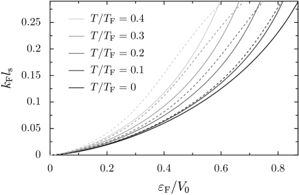
Figure 4: $k_{\rm F}l_{\rm s}$ from (55) as a function of $\varepsilon_{\rm F}/V_{0}$ at zero temperature (black line) and for finite temperatures (solid gray lines). The dashed lines result from the numerical integration of (48). In the figure, $T/T_{\rm F}$ increases from bottom to top.

IV.3 Number of spill-out electrons: Semiclassics vs. LDA

In this section, we compare our semiclassical evaluation of the spill-out effect at zero temperature with LDA calculations on spherical sodium nanoparticles. One possible way to estimate $N_{\rm out}$ is to use the LDA, which allows to compute the spherically symmetric self-consistent electronic ground-state density for nanoparticles with closed electronic shells. Integrating the density outside the nanoparticle then yields an approximation to $N_{\rm out}$, and thus to $l_{\rm s}$ according to (54). An estimation of the spill-out length from (55) by means of our semiclassical theory at zero temperature gives $l_{\rm s}\simeq 0.2\,a_{0}$ for sodium nanoparticles, while Madjet and collaborators obtained on the basis of Kohn-Sham and Hartree-Fock calculations $l_{\rm s}$ around $0.55\,a_{0}$ for clusters of size $N=8$–$196$. madjet With our LDA calculations, we obtain $l_{\rm s}$ of the order of $0.45\,a_{0}$ for all closed-shell sizes between $N=8$ and $N=1760$ (see the squares in Fig. 5).

Figure 5: Spill-out length $l_{\rm s}$ at $T=0$ in units of the Bohr radius $a_{0}$ as a function of the total number of electrons $N$, after (55) (solid line) for sodium nanoparticles. The dashed line is twice the result of (55), and is obtained considering the effective radius $a_{\rm eff}$ for the approximated self-consistent potential, namely $V(r)=V_{0}\Theta(r-a_{\rm eff})$. The squares result from LDA calculations.

The fact that the semiclassical spill-out length is significantly smaller than that of LDA is a consequence of our assumption of a step-like potential for $V$. Indeed, the LDA self-consistent potential $V$ shown in Fig. 6 deviates from the form $V(r)=V_{0}\Theta(r-a)$ that we have used. As one can see in Fig. 6, the Fermi level does not coincide with $V(a)$. Defining the effective radius of the nanoparticle for the spill-out effect by means of $V(a_{\rm eff})=\varepsilon_{\rm F}$, it seems appropriate to approximate the self-consistent potential by $V(r)=V_{0}\Theta(r-a_{\rm eff})$. An estimation from our LDA calculations gives $a_{\rm eff}\simeq a+l_{\rm s}$ for all sizes between $N=8$ and $N=1760$. Using this effective radius in (49) does not change our results for $N_{\rm out}$ and $l_{\rm s}$ since $a\gg l_{\rm s}$. However, the spill-out length is defined from the geometrical radius $a$ of the ionic jellium background of the nanoparticle. Since $a_{\rm eff}\simeq a+l_{\rm s}$, it actually yields an effective spill-out length $l_{\rm s}^{\rm eff}\approx 2l_{\rm s}$ and approximately doubles our result for $N_{\rm out}$. The improved $T=0$ result for the spill-out length is represented by the dashed line in Fig. 5. It yields good agreement with the spill-out length as deduced from the LDA calculations (squares in Fig. 5). Note that there is no need to consider an effective radius of the nanoparticle in the calculation of the resonance width presented in Sec. III. Indeed, the linewidth $\gamma$ scales as $1/a$. Replacing $a$ by an effective radius for the linewidth $\gamma$ would thus only lead to higher-order corrections.

Figure 6: Detail of the LDA self-consistent potential $V$ close to the boundary of the cluster as a function of the radial coordinate $r$ for a sodium nanoparticle containing $N=1760$ valence electrons. The radius $a$ is indicated by the vertical dotted line, and the effective radius defined by $V(a_{\rm eff}\simeq a+l_{\rm s})=\varepsilon_{\rm F}$ is indicated by the dashed line. The Fermi level corresponds to the horizontal dashed line.

IV.4 Redshift of the surface plasmon resonance

We now examine the redshift of the surface plasmon resonance by means of TDLDA calculations. In Fig. 7, we show the frequencies deduced from the LDA number of spill-out electrons for various closed-shell nanoparticle sizes between $N=8$ and $N=1760$, where $N_{\rm out}$ is incorporated according to (4) (squares). The dashed line is our semiclassical result from (53) with (4), where we have taken into account the effective radius for the self-consistent potential, as discussed in the preceding section. We see that our analytical expression for the spill-out is in a good agreement with the LDA calculations, and that the redshift is increasing with decreasing size as predicted by (53).

Figure 7: Surface plasmon frequency as a function of the number $N$ of valence electrons in the nanoparticle. Squares: $\tilde{\omega}_{\rm M}/\omega_{\rm M}$, frequencies deduced from the LDA number of spill-out electrons according to (4). Dashed line: semiclassical evaluation of (53) with (4). Dots: $\omega_{\rm sp}/\omega_{\rm M}$, frequencies obtained by fitting the TDLDA absorption curves with a Mie-type cross section. deheer Dotted line: linear fit to the dots. Solid line: sum of the spill-out effect (dashed line) and the environment-induced redshift of the resonance (64). All results shown here are at zero temperature for the case of sodium. The points shown represent all closed shell sizes between $N=8$ and $N=1760$.

Alternatively the resonance frequency can be extracted directly from the absorption cross section $\sigma(\omega)$ defined in (3) and calculated from the TDLDA response function (see Fig. 1). An upper bound for the resonance energy is given by the root mean square brack ; bohigas

$$\sqrt{\langle\omega^{2}\rangle}=\sqrt{\frac{\int_{0}^{\infty}{\rm d}\omega\ \omega^{2}\sigma(\omega)}{\int_{0}^{\infty}{\rm d}\omega\ \sigma(\omega)}},$$ (56)

providing a lower bound for the redshift of the surface plasmon frequency from the Mie value. In the spherical jellium model, the frequency deduced from (56) coincides with $\tilde{\omega}_{\rm M}$, brack ; bertsch_ekardt the Mie frequency redshifted by the spill-out effect (4). We have checked with our TDLDA calculations that the frequencies deduced from $N_{\rm out}$, i.e., from the electronic ground-state self-consistent density correspond to the frequencies obtained from (56), up to the numerical error. At zero temperature, the TDLDA thus fulfills the sum rule brack $\sqrt{\langle\omega^{2}\rangle}=\tilde{\omega}_{\rm M}$.

The dots in Fig. 7 represent the maxima $\omega_{\rm sp}$ of the absorption curves obtained by fitting the TDLDA results with a Mie-type cross section. deheer It is clear from Fig. 7 that the frequency obtained by (4) from the number of spill-out electrons (squares) overestimates the resonance frequency $\omega_{\rm sp}$ (see also Fig. 1). HF It has been noticed in Ref. reiners, that the spill-out effect is not sufficient to describe the experimentally observed resonance frequency.

In the following section, we propose to interpret the discrepancy between $\omega_{\rm sp}$ given by the TDLDA and $\tilde{\omega}_{\rm M}$ deduced from the spill-out by means of the coupling of the surface plasmon mode to electron-hole excitations. This coupling results in a shift of the surface plasmon frequency which adds to the effect of the spill-out.

V Environment-induced frequency shift

In the absence of the coupling $H_{\rm c}$, the energy of the $n^{\rm th}$ eigenstate of the center-of-mass system is given by the eigenenergies ${\cal E}^{(0)}_{n}=n\hbar\tilde{\omega}_{\rm M}$ of $H_{\rm cm}$ given in (17). However, the coupling Hamiltonian (19) perturbs the eigenstates of $H_{\rm cm}$. The leading contribution to the resulting shift of the eigenenergies ${\cal E}^{(0)}_{n}$ is determined using perturbation theory in $H_{\rm c}$. While the first order does not contribute due to the selection rules contained in the coupling (19), there are four second-order processes involving virtual particle-hole pairs. In addition to the two resonant processes mentioned in Sec. III.1, i.e., decay into the ground state with creation of a particle-hole pair and excitation to a higher state accompanied by the annihilation of a particle-hole pair, there exist also two antiresonant processes. A plasmon can be excited to a higher collective state by creating a particle-hole pair, or a plasmon can decay by destroying a particle-hole pair. Taking into account all four processes, we obtain the resonance energy to second order in the coupling

$$\hbar\omega_{\rm sp}={\cal E}^{(2)}_{1}-{\cal E}^{(2)}_{0}=\hbar\left(\tilde{\omega}_{\rm M}-\delta\right)$$ (57)

with the frequency shift

$$\delta=\frac{1}{\hbar}\sum_{\begin{subarray}{c}F_{\rm cm}\\ I_{\rm rel},F_{\rm rel}\end{subarray}}P_{I_{\rm rel}} \left(\frac{\left|\langle F_{\rm cm},F_{\rm rel}|H_{\rm c}|1_{\rm cm},I_{\rm rel}\rangle\right|^{2}}{\varepsilon_{F_{\rm cm}}-\hbar\tilde{\omega}_{\rm M}+\varepsilon_{F_{\rm rel}}-\varepsilon_{I_{\rm rel}}}\right.$$

$$\left.-\frac{\left|\langle F_{\rm cm},F_{\rm rel}|H_{\rm c}|0_{\rm cm},I_{\rm rel}\rangle\right|^{2}}{\varepsilon_{F_{\rm cm}}+\varepsilon_{F_{\rm rel}}-\varepsilon_{I_{\rm rel}}}\right),$$ (58)

where we use the same notations as in Sec. III.1. Writing explicitly the coupling Hamiltonian $H_{\rm c}$ (19) in the preceding expression, we obtain

$$\delta=\frac{2}{\hbar^{2}}{\cal P}\sum_{\alpha\beta}\left[1-f(\varepsilon_{\alpha})\right]f(\varepsilon_{\beta})\left|\Lambda d_{\alpha\beta}\right|^{2}\frac{\omega_{\alpha\beta}}{\omega_{\alpha\beta}^{2}-\tilde{\omega}_{\rm M}^{2}}.$$ (59)

Here, $\cal P$ denotes the Cauchy principal value. The resonance frequency $\omega_{\rm sp}$ (57) thus contains a correction with respect to the value induced by the spill-out effect. As we will show, the shift $\delta$ is positive, and thus redshifts the plasmon resonance from $\tilde{\omega}_{\rm M}$.

According to (24) and (59), the energy shift $\delta$ is related to the function $\Sigma(\omega)$ through the Kramers-Kronig relation

$$\delta=\frac{1}{\pi}{\cal P}\int_{-\infty}^{+\infty}{\rm d}\omega\frac{\omega\Sigma(\omega)}{\omega^{2}-\tilde{\omega}_{\rm M}^{2}}.$$ (60)

In (60), the frequency $\tilde{\omega}_{\rm M}$ appearing in the denominator can be replaced by $\omega_{\rm M}$. Indeed, the function $\Sigma(\omega)$ of (34) is proportional to $1/k_{\rm F}a$. Thus, taking into account the spill-out effect in the evaluation of $\delta$ would yield higher order terms in powers of $1/k_{\rm F}a$, that we neglect in the semiclassical limit. Furthermore, we have to restrict the integral over the frequency $\omega$ by introducing the cutoff $\omega_{\rm c}$ discussed in Sec. III.1. It arises from the fact that the particle-hole pairs that participate to $\delta$ in (59) belong to the high-energy sector of the RPA Hilbert space, while the surface plasmon excitation is the superposition of particle-hole pairs of the restricted low-energy subspace. The TDLDA absorption cross section shows a large excitation peak at the frequency $\omega_{\rm sp}$ which supports almost all of the dipole strength. This peak is surrounded by particle-hole excitations that become noticeable for frequencies larger than $\sim\omega_{\rm M}-\eta\gamma$, where $\eta$ is a constant of the order of unity. Thus for the purpose of calculating the integral (60) we can take the cutoff at $\omega_{\rm M}-\eta\gamma$ and approximate

$$\delta\simeq\frac{1}{\pi}{\cal P}\int_{\omega_{\rm M}-\eta\gamma}^{+\infty}{\rm d}\omega\frac{\omega\Sigma(\omega)}{\omega^{2}-\omega_{\rm M}^{2}}.$$ (61)

For frequencies $\omega$ larger than $\omega_{\rm M}-\eta\gamma$, the function $g$ appearing in (34) can be replaced by its asymptotic expansion for $\varepsilon_{\rm F}\ll\hbar\omega$,

$$g\left(x,\frac{T}{T_{\rm F}}\right)\simeq\left[\frac{8}{15}+\frac{2\pi^{2}}{9}\left(\frac{T}{T_{\rm F}}\right)^{2}\right]\sqrt{x}.$$ (62)

Inserting this expression into (61), and performing the remaining integral over $\omega$ in the semiclassical limit $k_{\rm F}a\gg 1$, we arrive at

$$\delta\simeq\frac{3v_{\rm F}}{4a} \sqrt{\frac{\varepsilon_{\rm F}}{\hbar\omega_{\rm M}}}\left[\ln{\left(\frac{4\omega_{\rm M}}{\eta\gamma}\right)}-\frac{\pi}{2}-\frac{4}{3}\right]$$

$$\times\left[\frac{4}{15\pi}+\frac{\pi}{9}\left(\frac{T}{T_{\rm F}}\right)^{2}\right].$$ (63)

We remark that the dependence of this result on the cutoff is only logarithmic.

Inserting our expression (38) for the linewidth $\gamma$, we obtain to second order in $T/T_{\rm F}$

$$\delta=\frac{3v_{\rm F}}{4a}j\left(\frac{\varepsilon_{\rm F}}{\hbar\omega_{\rm M}},\frac{T}{T_{\rm F}}\right)$$ (64)

where

$$j\left(x,\frac{T}{T_{\rm F}}\right)=j_{0}(x)+j_{2}(x)\left(\frac{T}{T_{\rm F}}\right)^{2},$$ (65)

with

$$j_{0}(x)=\frac{4\sqrt{x}}{15\pi}\left[\ln{\left(\frac{8k_{\rm F}a}{3\eta xg_{0}(x)}\right)}-\frac{\pi}{2}-\frac{4}{3}\right]$$ (66)

and

$$j_{2}(x)=\frac{\pi\sqrt{x}}{9}\left[\ln{\left(\frac{8k_{\rm F}a}{3\eta xg_{0}(x)}\right)}-\frac{\pi}{2}-\frac{4}{3}-\frac{12}{5\pi^{2}}\frac{g_{2}(x)}{g_{0}(x)}\right].$$ (67)

The functions $g_{0}$ and $g_{2}$ are defined in (36) and (III.2), respectively. While the linewidth (38) goes as $1/a$, the frequency shift scales as $1/a$ up to a logarithmic factor. This redshift increases with temperature and adds to the redshift arising from the spill-out effect discussed in Sec. IV.

The importance of the shift $\delta$ can be seen in Fig. 7. There, the position of the surface plasmon resonance peak for sodium clusters calculated from TDLDA (dots) is in qualitative agreement with our semiclassical result (solid line) taking into account the shift $\delta$ and the spill-out (see Eqs. 4 and 53 in Sec. IV). footnote_TDLDA In Fig. 7, we have used $\eta=1/2$ for the frequency cutoff in (61). Our approximate expression for $\delta$ does not allow us to obtain a quantitative agreement with the position $\omega_{\rm sp}$ of the resonance frequency shown by the dots. This is not surprising considering the approximations needed in order to derive an analytical result. First, the expression for $\delta$ is based on our result (34) for $\Sigma(\omega)$ which was derived under the assumption of perfectly confined electronic states. Thus, the delocalized self-consistent single-particle states have not been accurately treated in the calculation of $\delta$. Second, the cutoff introduced above is a rough estimate of the energy beyond which particle-hole excitations couple to the surface plasmon. Despite those approximations, our estimate implies an increase of the redshift beyond that caused by the spill-out (dashed line in Fig. 7). Comparing the two effects leading to a redshift of the surface plasmon frequency, we find that they have the same size and temperature dependence, and are of the same order of magnitude. Therefore, one has to take into account both contributions in quantitative descriptions of the surface plasmon frequency.

For zero temperature, the shift $\delta$ has also been considered in Refs. gerchikov, and hagino, . The authors of Ref. gerchikov, have used the separation of the collective center-of-mass motion from the relative coordinates. Their coupling between the two subsystems which is only nonvanishing outside the nanoparticle leads to a shift that they have numerically evaluated by means of the RPA plus exchange in the case of small charged sodium clusters. In Ref. hagino, , the authors assumed a certain expression for the coupling, and a variational RPA calculation was used to obtain an analytical expression of the environment-induced redshift. In contrast to our findings, Refs. gerchikov, and hagino, obtained a shift $\delta$ proportional to the number of spill-out electrons.

For very small clusters ($N$ between $8$ and $92$), a nonmonotonic behavior of the resonance frequency as a function of the size of the nanoparticle has been observed experimentally. reiners This behavior is in qualitative agreement with our numerical calculations (see dots in Fig. 7) and can be understood in the following way. We have shown in Refs. weick, and molina, that the linewidth of the surface plasmon resonance presents oscillations as a function of the size of the nanoparticle. Furthermore, we have shown in this section that the linewidth and the environment-induced shift are related through the Kramers-Kronig transform (60). Thus, the shift $\delta$ should also present oscillations as a function of the size of the cluster. This is in contrast to the spill-out effect discussed in Sec. IV where the oscillating character of the DOS leads to a vanishing contribution, as confirmed by the LDA calculations (see squares in Fig. 7). Those significantly different behaviors could permit to distinguish between the two mechanisms contributing to the redshift of the surface plasmon frequency with respect to the classical Mie value.

Using temperature-dependent TDLDA calculations, Hervieux and Bigot hervieux have recently found a nonmonotonic behavior of the energy shift of the surface plasmon frequency as a function of the temperature for a given nanoparticle size. They observed a redshift of the surface plasmon resonance up to a certain critical temperature (e.g., $1000\,\mathrm{K}$ and $2500\,\mathrm{K}$ for Na₁₃₈ and Na${}_{139}^{+}$, respectively), followed by a blueshift of the resonance at higher temperatures. This behavior is not present in our theory. The authors of Ref. hervieux, attribute the nonmonotonic temperature dependence to the coupling of the surface plasmon to bulklike extended states in the continuum, which causes a blueshift, as one can expect for a bulk metal. However, we have restricted ourselves to low temperatures compared to the work function of the nanoparticle, where we can neglect those extended states in the evaluation of the spill-out. The critical temperature of a thousand degrees is much smaller than the Fermi temperature for metals, such that our treatment should remain a good approximation.

VI Time evolution of the optical transmission in a pump-probe configuration

We now examine the experimental consequences of the temperature dependence of the Landau damping linewidth (38) and of the energy shifts induced by the spill-out (Eqs. 4 and 53) and by the electronic environment (64).

We focus on the absorption cross section defined in (3). Assuming it to be of the Breit-Wigner form, we have

$$\sigma(\omega,T)=s(a)\frac{\gamma(T)/2}{\left[\omega-\omega_{\rm sp}(T)\right]^{2}+\left[\gamma(T)/2\right]^{2}},$$ (68)

where $\omega_{\rm sp}(T)$ is the temperature-dependent resonance frequency of the surface plasmon excitation given in (57). $s(a)$ is a size-dependent normalization prefactor. For the spill-out, we consider the effective radius discussed in Sec. IV.3 which doubles the results of (53).

Unfortunately, to the best of our knowledge, systematic experimental investigations of the shape of the absorption cross section as a function of temperature are not available. However, an indirect approach is offered by pump-probe experiments, bigot ; delfatti where the nanoparticles are excited by an intense laser pulse. After a given time delay, the system is probed with a weak laser field, measuring the transmission ${\cal T}$ of the nanoparticles. After the excitation of a surface plasmon, its energy is transferred on the femtosecond timescale to the electronic environment, resulting in the heating of the latter. On a much longer timescale of typically a picosecond, the equilibration of the electrons with the phonon heat bath results in the decrease of the temperature of the electronic system with time. Such a process is not included in our theory.

An experimentally accessible quantity bigot ; delfatti is the differential transmission $\Delta{\cal T}/{\cal T}=({\cal T}_{\rm on}-{\cal T}_{\rm off})/{\cal T}_{\rm off}$, i.e., the normalized difference of transmissions with and without the pump laser field. It is related to the absorption cross section by means of

$$\frac{\Delta{\cal T}}{\cal T}(\omega,T)=-\frac{3}{2\pi a^{2}}\left[\sigma(\omega,T)-\sigma(\omega,T_{\rm amb})\right],$$ (69)

$T_{\rm amb}$ being the ambient temperature. The relation (69) between transmission and absorption holds provided that the reflectivity of the sample can be neglected, which is the case in most of the experimental setups. The differential transmission can be viewed in two different ways. For a fixed time delay between the pump and the probe pulses, it is sensitive to the energy provided by the pump laser which is transferred to the electronic environment via the surface plasmon, and thus to the temperature of the heat bath. Alternatively, for a given pump intensity, increasing the time delay between the pump and the probe scans the relaxation process of the electronic system as the bath temperature decreases.

Figure 8: Differential transmission $\Delta{\cal T}/{\cal T}$ as a function of the probe energy $\hbar\omega$ for increasing temperatures, resulting from increasing pump intensities and a fixed delay between pump and probe (or by decreasing the time delay at a fixed pump intensity). The presented results are for a sodium nanoparticle with a radius $a=2\,\mathrm{nm}$.

In Fig. 8, we present the differential transmission of (69) for a sodium nanoparticle of radius $a=2\,\mathrm{nm}$, which has a strong surface plasmon resonance around $3.5\,\mathrm{eV}$. We see that as the temperature of the electronic system increases, $\Delta{\cal T}/{\cal T}$ becomes more and more pronounced since both, the linewidth and the redshift of the resonance frequency in (68) increase with temperature. Similar results are observed in experiments, bigot ; delfatti where the amplitude of $\Delta{\cal T}/{\cal T}$ is observed to decrease as a function of the time delay between the pump and the probe laser fields. This is accompanied by the blueshift of the crossing of the differential transmission curves with the zero line as the time delay increases. Moreover, the asymmetry of $\Delta{\cal T}/{\cal T}$ is observed in the experiments and obtained in our calculations.

Our results could provide a possibility to fit the experimental results on metallic nanoparticles excited by a pump laser field in order to extract the temperature, and thus could assist in analyzing the relaxation process.

VII Conclusion

The role of the electronic environment on the surface plasmon resonance in metallic nanoparticles has been analyzed in this work. By means of a separation into collective and relative coordinates for the electronic system, we have shown that the coupling to particle-hole excitations leads to a finite lifetime as well as a frequency shift of the collective surface plasmon excitation. The size and temperature dependence of the linewidth of the surface plasmon has been investigated by means of a semiclassical evaluation within the mean-field approximation, together with a low-temperature expansion. In addition to the well-known size dependence of the linewidth, we have demonstrated that an increase in temperature leads to an increasing width of the resonance. The effect of finite temperature has been found to be weak, in qualitative agreement with the experimental results.

We have analyzed the spill-out effect arising from the electron density outside the nanoparticle. Our semiclassical analysis has led to a good agreement with LDA calculations. In order to achieve this, it was necessary to introduce an effective radius of the nanoparticle which accounts for the details of the self-consistent mean-field potential. The ratio of spill-out electrons over the total number as well as the resulting redshift of the surface plasmon frequency scale inversely with the size of the nanoparticle. The spill-out-induced redshift was shown, by means of a Sommerfeld expansion, to increase with the temperature.

We have demonstrated that the coupling between the electronic center of mass and the relative coordinates results in an additional redshift of the surface plasmon frequency. This effect is of the same order as the redshift induced by the spill-out effect and presents a similar size and temperature dependence. Thus it has to be taken into account in the description of numerical and experimental results. Our semiclassical theory predicts that for the smallest sizes of nanoparticles, the environment-induced redshift should exhibit a nonmonotonic behavior as a function of the size, as confirmed by numerical calculations. This is not the case for the redshift caused by the spill-out effect, and thus permits to distinguish between the two effects.

Our theory of the thermal broadening of the surface plasmon resonance, together with the temperature dependence of the resonance frequency, qualitatively explains the observed differential transmission that one measures in time-resolved pump-probe experiments. Our findings could open the possibility to analyze relaxation processes in excited nanoparticles.

Appendix A Low-temperature expansion for integrals involving two Fermi functions

In this appendix, we calculate the function $\cal F$ defined in (32), which involves the integral of two Fermi distributions. Integrating (32) by parts yields

$${\cal F}(\mu,\hbar\omega)=\int_{\hbar\omega}^{\infty}{\rm d}\varepsilon\left(-\frac{{\rm d}F}{{\rm d}\varepsilon}\right){\cal H}\left(\frac{\varepsilon}{\hbar\omega}\right)$$ (70)

with

$${\cal H}(x)=\int_{1}^{x}{\rm d}x^{\prime}H(x^{\prime}),$$ (71)

the function $H$ being defined in (33). In (70), we have introduced the notation $F(\varepsilon)=\left[1-f(\varepsilon)\right]f(\varepsilon-\hbar\omega)$. In the low-temperature limit $\hbar\omega\gg k_{\rm B}T$, we get

$$-\frac{{\rm d}F}{{\rm d}\varepsilon}\approx-\beta\frac{{\rm e}^{\beta(\varepsilon-\mu)}}{\left[{\rm e}^{\beta(\varepsilon-\mu)}+1\right]^{2}}+\beta\frac{{\rm e}^{\beta(\varepsilon-\hbar\omega-\mu)}}{\left[{\rm e}^{\beta(\varepsilon-\hbar\omega-\mu)}+1\right]^{2}},$$ (72)

which corresponds to two peaks of opposite sign centered at $\varepsilon=\mu$ and at $\varepsilon=\mu+\hbar\omega$. It is therefore helpful to expand in (70) the function ${\cal H}$ around $\varepsilon=\mu$ and $\varepsilon=\mu+\hbar\omega$. For low temperatures and for $|\hbar\omega-\mu|\gtrsim k_{\rm B}T$, we obtain

$${\cal F}(\mu,\hbar\omega)\simeq{\cal H}\left(1+\frac{\mu}{\hbar\omega}\right)-{\cal H}\left(\frac{\mu}{\hbar\omega}\right)\Theta(\mu-\hbar\omega)$$ (73)

$$+\frac{\pi^{2}}{6}\left(\frac{k_{\rm B}T}{\hbar\omega}\right)^{2}\left[H^{\prime}\left(1+\frac{\mu}{\hbar\omega}\right)-H^{\prime}\left(\frac{\mu}{\hbar\omega}\right)\Theta\left(\mu-\hbar\omega\right)\right]$$

where $H^{\prime}$ denotes the derivative of $H$. This treatment is appropriate for all values of $\omega$, except in a range of order $k_{\rm B}T$ around $\mu$. There, the nonanalyticity of $\cal H$ has to be properly accounted forthesis since for $x$ near $1$, ${\cal H}(x)\simeq(16/15)(x-1)^{5/2}$. At $\hbar\omega=\mu$, an additional term thus appears, and

$${\cal F}(\mu,\mu)\simeq{\cal H}(2)+\frac{\pi^{2}}{6}\left(\frac{k_{\rm B}T}{\hbar\omega}\right)^{2}H^{\prime}(2)-C\left(\frac{k_{\rm B}T}{\hbar\omega}\right)^{5/2}$$ (74)

with

$$C=\int_{0}^{\infty}{\rm d}x\frac{{\rm e}^{x}x^{5/2}}{\left({\rm e}^{x}+1\right)^{2}}\approx 3.07.$$ (75)

In order to pursue the evaluation of (73), we need to determine the chemical potential $\mu$. Since the DOS of (30), once summed over $l$ and $m$ yields weick the three-dimensional bulk DOS proportional to $\sqrt{\varepsilon}$, we can use the standard Sommerfeld expression for the chemical potential of free fermions. ashcroft We thus get for $|\hbar\omega-\mu|\gtrsim k_{\rm B}T$

$${\cal F}(\mu,\hbar\omega) \simeq\int_{\max{(\varepsilon_{\rm F},\hbar\omega)}}^{\varepsilon_{\rm F}+\hbar\omega}\frac{{\rm d}\varepsilon}{\hbar\omega}H\left(\frac{\varepsilon}{\hbar\omega}\right)+\frac{\pi^{2}}{6}\frac{\varepsilon_{\rm F}}{\hbar\omega}\left(\frac{T}{T_{\rm F}}\right)^{2}$$

$$\times\bigg{\{}\frac{\varepsilon_{\rm F}}{\hbar\omega}\left[H^{\prime}\left(1+\frac{\varepsilon_{\rm F}}{\hbar\omega}\right)-H^{\prime}\left(\frac{\varepsilon_{\rm F}}{\hbar\omega}\right)\Theta\left(\varepsilon_{\rm F}-\hbar\omega\right)\right]$$

$$\hskip 11.38092pt-\frac{1}{2}\left[H\left(1+\frac{\varepsilon_{\rm F}}{\hbar\omega}\right)-H\left(\frac{\varepsilon_{\rm F}}{\hbar\omega}\right)\Theta\left(\varepsilon_{\rm F}-\hbar\omega\right)\right]\bigg{\}},$$ (76)

where $T_{\rm F}$ is the Fermi temperature. Inserting the result (A) into (31), and using the expression (33) for $H$, we finally obtain (34).

References

- (1) W. A. de Heer, Rev. Mod. Phys. 65, 611 (1993).
- (2) M. Brack, Rev. Mod. Phys. 65, 677 (1993).
- (3) U. Kreibig and M. Vollmer, Optical Properties of Metal Clusters (Springer-Verlag, Berlin, 1995).
- (4) W. A. de Heer, K. Selby, V. Kresin, J. Masui, M. Vollmer, A. Châtelain, and W. D. Knight, Phys. Rev. Lett. 59, 1805 (1987).
- (5) C. Bréchignac, P. Cahuzac, N. Kebaïli, J. Leygnier, and A. Sarfati, Phys. Rev. Lett. 68, 3916 (1992).
- (6) H. Haberland, B. von Issendorff, J. Yufeng, and T. Kolar, Phys. Rev. Lett. 69, 3212 (1992).
- (7) C. Bréchignac, P. Cahuzac, J. Leygnier, and A. Sarfati, Phys. Rev. Lett. 70, 2036 (1993).
- (8) T. Reiners, W. Orlik, C. Ellert, M. Schmidt, and H. Haberland, Chem. Phys. Lett. 215, 357 (1993).
- (9) T. Reiners, C. Ellert, M. Schmidt, and H. Haberland, Phys. Rev. Lett. 74, 1558 (1995).
- (10) W. Ekardt, Phys. Rev. Lett. 52, 1925 (1984); Phys. Rev. B 32, 1961 (1985).
- (11) M. Barma and V. Subrahmanyam, J. Phys.: Condens. Matter 1, 7681 (1989).
- (12) C. Yannouleas and R. A. Broglia, Ann. Phys. (N.Y.) 217, 105 (1992).
- (13) G. F. Bertsch and R. A. Broglia, Oscillations in Finite Quantum Systems (Cambridge University Press, Cambridge, 1994).
- (14) M. Madjet, C. Guet, and W. R. Johnson, Phys. Rev. A 51, 1327 (1995).
- (15) D. Boyer, P. Tamarat, A. Maali, B. Lounis, and M. Orrit, Science 297, 1160 (2002); L. Cognet, C. Tardin, D. Boyer, D. Choquet, P. Tamarat, and B. Lounis, PNAS 100, 11350 (2003).
- (16) M. Dahan, S. Lévi, C. Luccardini, P. Rostaing, B. Riveau, and A. Triller, Science 302, 442 (2003).
- (17) B. Lamprecht, J. R. Krenn, A. Leitner, and F. R. Aussenegg, Appl. Phys. B 69, 223 (1999).
- (18) F. Stietz, J. Bosbach, T. Wenzel, T. Vartanyan, A. Goldmann, and F. Träger, Phys. Rev. Lett. 84, 5644 (2000).
- (19) J. Bosbach, C. Hendrich, F. Stietz, T. Vartanyan, and F. Träger, Phys. Rev. Lett. 89, 257404 (2002).
- (20) T. Klar, M. Perner, S. Grosse, G. von Plessen, W. Spirkl, and J. Feldmann, Phys. Rev. Lett. 80, 4249 (1998).
- (21) C. Sönnichsen, T. Franzl, T. Wilk, G. von Plessen, and J. Feldmann, New J. Phys. 4, 93.1 (2002).
- (22) A. Arbouet, D. Christofilos, N. Del Fatti, F. Vallée, J. R. Huntzinger, L. Arnaud, P. Billaud, and M. Broyer, Phys. Rev. Lett. 93, 127401 (2004).
- (23) M. A. van Dijk, M. Lippitz, and M. Orrit, Phys. Rev. Lett. 95, 267406 (2005).
- (24) S. Berciaud, L. Cognet, G. A. Blab, and B. Lounis, Phys. Rev. Lett. 93, 257402 (2004); S. Berciaud, L. Cognet, P. Tamarat, and B. Lounis, Nano Lett. 5, 515 (2005).
- (25) A. Kawabata and R. Kubo, J. Phys. Soc. Jpn. 21, 1765 (1966).
- (26) C. Yannouleas, Nucl. Phys. A 439, 336 (1985).
- (27) G. F. Bertsch, Comput. Phys. Commun. 60, 247 (1990).
- (28) L. G. Gerchikov, C. Guet, and A. N. Ipatov, Phys. Rev. A 66, 053202 (2002).
- (29) G. Weick, R. A. Molina, D. Weinmann, and R. A. Jalabert, Phys. Rev. B 72, 115410 (2005).
- (30) K. Hagino, G. F. Bertsch, and C. Guet, Nucl. Phys. A 731, 347 (2004).
- (31) C. Cohen-Tannoudji, J. Dupont-Roc, and G. Grynberg, Atom-Photon Interactions: Basic Processes and Applications (Wiley-VCH, New York, 1992).
- (32) J.-Y. Bigot, V. Halté, J.-C. Merle, and A. Daunois, Chem. Phys. 251, 181 (2000).
- (33) N. Del Fatti, F. Vallée, C. Flytzanis, Y. Hamanaka, and A. Nakamura, Chem. Phys. 251, 215 (2000).
- (34) See, e.g., U. Weiss, Quantum Dissipative Systems (World Scientific, Singapore, 1993); T. Dittrich, P. Hänggi, G.-L. Ingold, B. Kramer, G. Schön, and W. Zwerger, Quantum Transport and Dissipation (Wiley-VCH, Weinheim, 1998), Chap. 4.
- (35) W. Kohn, Phys. Rev. 123, 1242 (1961).
- (36) R. A. Molina, D. Weinmann, and R. A. Jalabert, Phys. Rev. B 65, 155427 (2002); Eur. Phys. J. D 24, 127 (2003).
- (37) M. C. Gutzwiller, Chaos in Classical and Quantum Mechanics (Springer-Verlag, Berlin, 1990).
- (38) S. Link and M. A. El-Sayed, J. Phys. Chem. B 103, 4212 (1999).
- (39) R. H. Doremus, J. Chem. Phys. 40, 2389 (1964); J. Chem. Phys. 42, 414 (1965).
- (40) U. Kreibig, J. Phys. F 4, 999 (1974).
- (41) J. M. Pacheco and R. A. Broglia, Phys. Rev. Lett. 62, 1400 (1989).
- (42) G. F. Bertsch and D. Tománek, Phys. Rev. B 40, 2749 (1989).
- (43) L. Rodríguez-Sánchez, J. Rodríguez, C. Blanco, J. Rivas, and A. López-Quintela, J. Phys. Chem. B 109, 1183 (2005).
- (44) The energy required to ionize the nanoparticle is the work function plus the charging energy. This corresponds to a temperature of several . Therefore for reasonable temperatures, nanoparticles cannot be thermoionized.
- (45) N. W. Ashcroft and N. D. Mermin, Solid State Physics (Harcourt, Orlando, 1976).
- (46) is a constant which includes quantum mechanical corrections. See, e.g., M. Seidl and J. P. Perdew, Phys. Rev. B 50, 5744 (1994).
- (47) O. Bohigas, A. M. Lane, and J. Mortell, Phys. Rep. 51, 267 (1979).
- (48) G. Bertsch and W. Ekardt, Phys. Rev. B 32, 7659 (1985).
- (49) Within the jellium model, the LDA is not responsible for any underestimation of the number of spill-out electrons, as it has been shown using Hartree-Fock and RPA calculations. brack Our results show that the frequency shift induced by the electronic environment has to be taken into account in order to explain the above-mentioned discrepancy.
- (50) We can compare the semiclassical and numerical results since both approaches are based on the many-body Hamiltonian (5), and thus contain the same physical ingredients.
- (51) P.-A. Hervieux and J.-Y. Bigot, Phys. Rev. Lett. 92, 197402 (2004).
- (52) G. Weick, Ph. D. Thesis, Université Louis Pasteur (unpublished).