Efficient solution of Poisson’s equation with free boundary conditions

Abstract

Interpolating scaling functions give a faithful representation of a localized charge distribution by its values on a grid. For such charge distributions, using a Fast Fourier method, we obtain highly accurate electrostatic potentials for free boundary conditions at the cost of O(N logN) operations, where N is the number of grid points. Thus, with our approach, free boundary conditions are treated as efficiently as the periodic conditions via plane wave methods.

I Introduction

Solving Poisson’s equation

$$\nabla^{2}V=\rho\;,$$ (1)

to find the electrostatic potential $V$ arising from a charge distribution $\rho$ is a basic problem that can be found in nearly any field of physics and chemistry. It is therefore essential to have efficient solution methods for it.

A large variety of methods has been developed for systems of point particles interacting by electrostatic forces. Formally this problem can be considered as the solution of Poisson’s equation where the charge distribution is a sum of delta functions. The classical method for periodic boundary conditions is the Ewald method ewald . For large systems and free boundary conditions the Fast Multipole Method FMM is a powerful method due to its linear scaling with respect to the number of particles.

The FMM method has been generalized for continous systems where the charge density can be represented as a sum of Gaussians multiplied by a polynomial scuseria . This generalization exhibits linear scaling with respect to the volume but not with respect to the number of Gaussians at constant volume. It works well in the context of quantum chemistry calculations with medium size Gaussian basis sets where the charge density is naturally obtained in the required form but it is not a general purpose method.

For periodic boundary conditions and smoothly varying charge densities plane wave methods are simple and powerful because the Laplacian is a diagonal matrix in a plane wave representation. Given a Fourier representation of the charge density one can therefore obtain the potential simply by dividing each Fourier coefficient by $|{\bf k}|^{2}$, where ${\bf k}$ is the wavevector of the Fourier coefficient. If the charge density is originally given in real space a first Fast Fourier Transformation (FFT) is required to obtain its Fourier coefficients, and a second FFT is required to obtain the potential in real space from its Fourier coefficients. The overall scaling is therefore of order $N\log{N}$ where $N$ is the number of grid points.

Because of the simplicity of these plane wave methods various attempts have been made to generalize them to free boundary conditions. The most rudimentary method is just to take a very large periodic volume and to hope that the amplitude of the potential is nearly zero on the surface of the volume. Due to the long range of electrostatic forces this condition is however not fulfilled for volume sizes that are affordable with plane waves. Such as scheme is only possible if adaptive periodic wavelets are used oleg . In addition periodic boundary conditions do not permit to treat systems with monopoles and dipoles because for such systems no well defined solution exists under periodic boundary conditions. The first method to attack the problem in a systematic way was by Hockney Hockney.1970 . He proposed a Fourier approximation to the kernel

$$K(r)=\frac{1}{r}$$ (2)

of the Poisson equation. The method was intended for applications in plasma physics where no high accuracy is required. In other application such as electronic structure calculations high accuracy is required and the method is not optimal. For a spherical geometry the Fourier coefficients of the $\frac{1}{r}$ kernel can be calculated analytically. This is the basis of the simple and powerful method by Füsti-Molnar and Pulay Fusti-Molnar-Pulay.2002 . Its obvious restriction is that it is efficient only for spherical geometries. Another rather complicated method was proposed by Martyna and Tuckerman. This method gives high accuracy only in the center of the computational volume. It requires therefore artificially large simulation boxes which is numerically very expensive. All the above discussed methods use FFT’s at some point and have therfore a $O(N\log N)$ scaling.

In this paper we will describe a new Poisson solver for free boundary conditions on an uniform mesh. Contrary to Poisson solvers based on plane wave functions, our method is using interpolating scaling functions to represent the charge density. It is therefore from the beginning free of long range interactions between supercells, that falsify results if plane waves are used to describe non-periodic systems. Due to the convolutions we have to evaluate our method has a $N\log(N)$ scaling instead of the ideal linear scaling, Due to its small prefactor the method is however most efficient when dealing with localized densities such as can be found for example in the context of ab initio pseudo-potential electronic structure calculations using finite differences chelikowsky finite elements pask or plane waves for non-periodic systems.

II Interpolating scaling functions

Scaling functions arise in wavelet theory  daub . A scaling function basis set can be obtained from all the translations by a certain grid spacing $h$ of the mother wavelet centered at the origin. What distinguished scaling functions from other localized basis functions like finite elements is the refinement relation. The refinement relation establishes a relation between a scaling function $\phi(x-i)$ and the same scaling functions compressed by a factor of two, or, equivalently, between the scaling functions on a grid with grid spacing $h$ and another one with spacing $h/2$. For the scaling function centered a the origin, it reads

$$\phi(x)=\sum_{j=-m}^{m}h_{j}\>\phi(2x-j)$$ (3)

where the $h_{j}$’s are the elements of a filter that characterizes the wavelet family. An interpolating wavelet has in addition the property that it is equal to one at the origin and zero at all other integer points. Because of this property it is very simple to find the scaling function expansion coefficients of any function. The coefficients are just the values of the function to be expanded on the grid. $m$-th order interpolating scaling functions are generated by $m-1$-th order recursive interpolation lazy . Fig. 1 shows an 14-th order and 100-th order interpolating scaling function. Three-dimensional scaling functions can be obtained as the product of their one-dimensional counterparts

$$\Phi_{i_{1},i_{2},i_{3}}({\bf r}) =\phi_{i_{1}}(x)\>\phi_{i_{2}}(y)\>\phi_{i_{3}}(z)$$

$$=\phi(x-i_{1})\>\phi(y-i_{2})\>\phi(z-i_{3})$$ (4)

where ${\bf r}=(x,y,z)$. The points $i_{1},i_{2},i_{3}$ are the nodes of an uniform 3-dimensional mesh, with $i_{p}=1,\cdots,n_{p}$, $p=1,2,3$.

Continuous charge distributions are represented in numerical work typically by their values $\rho_{i,j,k}$ on a grid. It follows from the above described properties of interpolating scaling functions that the corresponding continous charge density is given by

$$\rho({\bf r})=\sum_{i_{1},i_{2},i_{3}}\rho_{i_{1},i_{2},i_{3}}\phi(x-i_{1})\>\phi(y-i_{2})\>\phi(z-i_{3})$$ (5)

The mapping of Eq. 5 between the discretized and continous charge distribution ensures that the first $m$ discrete and continous moments are identical for a $m$-th order interpolating wavelet family, i.e.

$$\sum_{i,j,k}i^{\ell_{1}}j^{\ell_{2}}k^{\ell_{3}}\>\rho_{i,j,k}=\int{\rm d}{\bf r}\>x^{\ell_{1}}y^{\ell_{2}}z^{\ell_{3}}\>\rho({\bf r})\;,$$ (6)

if $\ell_{1},\ell_{2},\ell_{3}<m$. The proof of this relation is given in the Appendix. Since the various multipoles of the charge distribution determine the major features of the potential the above equalities tell us that a scaling function representation gives the most faithful mapping between a continuous and discretized charge distribution for electrostatic problems.

Figure 1: Plots of interpolating scaling functions and wavelets of 14-th and 100-th order.

III Poisson’s equation in a basis set of interpolating scaling functions

As is well known the following integral equation gives the potential for free boundary conditions

$$V({\bf r})=\int{\rm d}{\bf r}^{\prime}\frac{1}{|{\bf r}-{\bf r}^{\prime}|}\rho({\bf r}^{\prime})\;.$$ (7)

We are interested in the values of the potential on the same grid that was used for the charge density. Denoting the potential on the grid point ${\bf r}_{j_{1},j_{2},j_{3}}=(x_{j_{1}},y_{j_{2}},z_{j_{3}})$ by $V_{j_{1},j_{2},j_{3}}=V({\bf r}_{j_{1},j_{2},j_{3}})$ we have

$$V_{j_{1},j_{2},j_{3}} =$$ (8)

$$=\sum_{i_{1},i_{2},i_{3}}\rho_{i_{1},i_{2},i_{3}}\int{\rm d}{\bf r}^{\prime}\frac{\phi_{i_{1}}(x^{\prime})\>\phi_{i_{2}}(y^{\prime})\>\phi_{i_{3}}(z^{\prime})}{|{\bf r}_{j_{1},j_{2},j_{3}}-{\bf r}^{\prime}|}\;.$$

The above integral defines the discrete kernel

$$K(i_{1},j_{1};i_{2},j_{2};i_{3},j_{3})=\\ =\int{\rm d}{\bf r}^{\prime}\phi_{i_{1}}(x^{\prime})\>\phi_{i_{2}}(y^{\prime})\>\phi_{i_{3}}(z^{\prime})\frac{1}{|{\bf r}_{j_{1},j_{2},j_{3}}-{\bf r}^{\prime}|}\;.$$ (9)

Since the problem is invariant under combined translations of both the source point $(i_{1},i_{2},i_{3})$ and the observation point $(j_{1},j_{2},j_{3})$ the kernel depends only on the difference of the indices

$$K(i_{1},j_{1};i_{2},j_{2};i_{3},j_{3})=K(i_{1}-j_{1},i_{2}-j_{2},i_{3}-j_{3})$$ (10)

and the potential $V_{j_{1},j_{2},j_{3}}$ can be obtained from the charge density $\rho_{i_{1},i_{2},i_{3}}$ by the following 3-dimensional convolution:

$$V_{j_{1},j_{2},j_{3}}=\sum_{i_{1},i_{2},i_{3}}K(i_{1}-j_{1},i_{2}-j_{2},i_{3}-j_{3})\rho_{i_{1},i_{2},i_{3}}\;.$$ (11)

Once the Kernel is available in Fourier space, this convolution can be evaluated with two FFTs at a cost of $O(N\log N)$ operations where $N=n_{1}\>n_{2}\>n_{3}$ is the number of 3-dimensional grid points. Since all the quantities in the above equation are real, real-to-complex FFT’s can be used to reduce the number of operations compared to the case where one would use ordinary complex-complex FFT’s. Obtaining the Kernel in Fourier space from the Kernel $K(j_{1},j_{2},j_{3})$ in real space requires another FFT.

It remains now to calculate the values of all the elements of the kernel $K(k_{1},k_{2},k_{3})$. Solving a 3-dimensional integral for each element would be much too costly and we use therefore a separable approximation of $1/r$ in terms of Gaussians Beylkin-Mohlenkamp.2002 ; harrison ,

$$\frac{1}{r}\simeq\sum_{k}\omega_{k}e^{-p_{k}r^{2}}\;.$$ (12)

In this way all the complicated 3-dimensional integrals become products of simple 1-dimensional integrals. Using $89$ Gaussian functions with the coefficients $\omega_{k}$ and $p_{k}$ suitably chosen, we can approximate $\frac{1}{r}$ with an error less than $10^{-8}$ in the interval $[10^{-9}\,,1]$. If we are interested in a wider range, e.g. a variable $R$ going from zero to $L$, we can use $r=\frac{R}{L}$:

$$\frac{L}{R} = \sum_{k}\omega_{k}e^{-\frac{p_{k}}{L^{2}}R^{2}}\;,$$ (13)

$$\frac{1}{R} = \frac{1}{L}\sum_{k}\omega_{k}e^{-P_{k}R^{2}}\;,$$ (14)

$$P_{k} = \frac{p_{k}}{L^{2}}\;.$$ (15)

With this approximation, we have that

$$K_{j_{1},j_{2},j_{3}}=\sum_{k=1}^{89}\omega_{k}K_{j_{1}}(p_{k})K_{j_{2}}(p_{k})K_{j_{3}}(p_{k})\;,$$ (16)

where

$$K_{j}(p_{k}) = \int\varphi_{j}(x)e^{-p_{k}x^{2}}{\rm d}x$$ (17)

$$= \int\varphi_{0}(x)e^{-p_{k}(x-j)^{2}}{\rm d}x\;.$$ (18)

So we only need to evaluate $89$ $\times$ $\max\left(\{n_{1},n_{2},n_{3}\}\right)$ integrals of the type

$$K_{j}(p)=\int\varphi_{0}(x)e^{-p(x-j)^{2}}{\rm d}x\;,$$ (19)

for some value of $p$ chosen between $3\cdot 10^{-5}$ and $3\cdot 10^{16}$.

The accuracy in calculating the integrals can be further improved by using the refinement relation for interpolating scaling functions 3.

From 19, we can evaluate $K_{i}(4p)$ as:

$$K_{i}(4p) = \int\varphi(x)e^{-4p(x-i)^{2}}{\rm d}x$$ (20)

$$= \frac{1}{2}\int\varphi(x/2)e^{-p(x-2i)^{2}}{\rm d}x$$ (21)

$$= \frac{1}{2}\sum_{j}h_{j}\int\varphi_{j}(x)e^{-p(x-2i)^{2}}{\rm d}x$$ (22)

$$= \frac{1}{2}\sum_{j}h_{j}K_{2i-j}(p)\;.$$ (23)

The best accuracy in evaluating numerically the integral is attained for $p<1$. For a fixed value of $p$ given by Eq. 12, the relation 23 is iterated $n=[\log_{4}(p)]$ times starting with $p_{0}=\frac{p}{4^{n}}$. So the numerical calculation of the integrals $K_{i}(p)$ is performed as follows: for each $p$, we compute the number $n$ of required recursions levels and calculate the integral $K_{i}(p_{0})$. The value of $n$ is chosen such that $p_{0}\simeq 1$ so we have a gaussian functions not too sharp. The evaluation of the interpolating scaling functions is fast on a uniform grid of points so we perform a simple summation over all the grid points. In Figure 2, we show that $1024$ points are enough to obtain machine precision. Note that the values of $K_{0}(p)$ vary over many orders of magnitude as shown in In Figure 2.

Figure 2: Plots of the value of $K_{0}(p)$ (top) and error of the integration defining its value (bottom) of for 1024 integration points for all the values of $p$ used in the tensor decomposition of $1/r$ in gaussian functions.

IV Numerical results and comparison with other methods

We have compared our method with the plane wave methods by Hockney Hockney.1970 and Martyna and Tuckerman Martyna-Tuckerman.1999 as implemented in the CPMD electronic structure program cpmd . As expected Hockney’s method does not allow to attain high accuracy. The method by Martyna and Tuckerman has a rapid exponential convergence rate which is characteristic for plane wave methods. Our new method has an algebraic convergence rate of $h^{m}$ with respect to the grid spacing $h$. By choosing very high order interpolating scaling functions we can get arbitrarily high convergence rates. Since convolutions are performed with FFT techniques the numerical effort does not increase as the order $m$ is increased. The accuracy shown in Figure 3 for the Martyna and Tuckerman method is the accuracy in the central part of the cube that has 1/8 of the total volume of the computational cell. Outside this volume errors blow up. So the main disadvantage of this method is that a very large computational volume is needed in order to obtain accurate results in a sufficiently large target volume. For this reason the less acurate Hockney method is generally prefered in the CPMD program hutter .

A strictly localized charge distribution, i.e. a charge distribution that is exactly zero outside a finite volume, can not be represented by a finite number of plane waves. This is an inherent contradiction in all the plane wave methods for the solution of Poisson’s equation under free boundary conditions. For the test shown in Figure 3 we used a Gaussian charge distribution whose potential can be calculated analytically. The Gaussian was embedded in a computational cell that was so large that the tails of the Gaussian were cut off at an amplitude of less than 1.e-16. A Gaussian can well be represented by a relatively small number of plane waves and so the above described problem is not important. For other localized charge distributions that are less smooth a finite Fourier representation is worse and leads to a spilling of the charge density out of the original localization volume. This will lead to inaccuracies in the potential.

Table 1 shows the required CPU time for a $128^{3}$ problem as a function of the number of processors on a Cray parallel computer. The parallel version is based on a parallel 3-dimensional FFT.

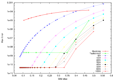
Figure 3: Accuracy comparison between our method with interpolating scaling functions of different orders and the Hockney of Martyna-Tuckerman method as implemented in CPMD. The accuracy of our method is finally limited by the accuracy of the expansion of Eq. 12 with 89 terms.

1	2	4	8	16	32	64
.92	.55	.27	.16	.11	.08	.09

Table 1: The elapsed time in seconds required on a Cray XT3 (based on AMD Opteron processors) to solve Poisson’s equation on a 128³ grid as a function of the number of processors. Since Poisson’s equation is typically solved many times, the time for setting up the Kernel is not included. Including the set up time of the Kernel increases the total timing by about 50 percent, since one additional FFT is needed.

A package for solving Poisson’s equation according to the method described here can be downloaded from www.unibas.ch/comphys/comphys/SOFTWARE

In conclusion, we have presented a method that allows to obtain the potential of a localized charge distribution under free boundary conditions with a $O(N\log N)$ scaling in a mathematically clean way. Even though our method has the same scaling behaviour as existing plane wave methods it is not a plane wave method in the sense that neither the charge density nor the potential are ever represented by plane waves. Instead interpolating scaling functions are used for the representation of the charge density.

We acknowledge interesting discussions with Reinhold Schneider and Robert Harrison. This work was supported by the European Commission within the Sixth Framework Programme through NEST-BigDFT (contract no. BigDFT-511815) and by the Swiss National Science Foundation. Research of G.B. was partially supported by DOE grant DE-FG02-03ER25583, DOE/ORNL grant 4000038129 and DARPA/ARO grant W911NF-04-1-0281. The timings were performed at the CSCS (Swiss Supercomputing Center) in Manno.

Appendix A

In the present Appendix we are going to prove Eq. (6): Let $\phi(x)$ be an interpolating scaling function of Deslariers-Dubuc, of the order $m$, and $\rho_{i_{1},i_{2},i_{3}}$ be a three-dimensional array of constant coefficients. Let, further,

$$\rho({\bf r})=\sum_{i_{1},i_{2},i_{3}}\rho_{i_{1},i_{2},i_{3}}\phi(x-i_{1})\phi(x-i_{2})\phi(x-i_{3}).$$ (24)

Then,

$$\sum_{i_{1},i_{2},i_{3}}i_{1}^{l_{1}}i_{2}^{l_{2}}i_{3}^{l_{3}}\rho_{i_{1},i_{2},i_{3}}=\int d{\bf r}x^{l_{1}}y^{l_{2}}z^{l_{3}}\rho({\bf r})$$ (25)

$${\rm if}\qquad 0\leq l_{1},\,l_{2},\,l_{3}<m$$

This follows from the fact, proven in reference beyl that the first $m$ moments of the scaling function obey the formula:

$$M_{l}=\int\phi(x)x^{l}{\rm d}x=\delta_{l},\qquad l=0,..,m-1$$ (26)

Shift the integration variable, we have

$$\int\phi(x-j)x^{l}{\rm d}x=\int\phi(t)(t+j)^{l}{\rm d}t=$$

$$= \int\phi(t)\sum_{p=0}^{l}C_{l}^{p}t^{p}j^{l-p}{\rm d}t=j^{l}$$

Then, inserting (24) into the right side of (25), we get:

$$\int{\rm d}{\bf r}x^{l_{1}}y^{l_{2}}z^{l_{3}}\rho({\bf r})=\int x^{l_{1}}y^{l_{2}}z^{l_{3}}\sum_{i_{1},i_{2},i_{3}}\rho_{i_{1},i_{2},i_{3}}\times$$

$$\times \phi(x-i_{1})\phi(x-i_{2})\phi(x-i_{3}){\rm d}{\bf r}=\sum_{i_{1},i_{2},i_{3}}\rho_{i_{1},i_{2},i_{3}}\times$$

$$\times \int x^{l_{1}}\phi(x-i_{1}){\rm d}x\int y^{l_{2}}\phi(y-i_{2}){\rm d}y\times$$

$$\times \int z^{l_{3}}\phi(z-i_{3}){\rm d}z=\sum_{i_{1},i_{2},i_{3}}\rho_{i_{1},i_{2},i_{3}}i_{1}^{l_{1}}i_{2}^{l_{2}}i_{3}^{l_{3}}$$

References

- (1) P. Ewald, Ann. Phys 64, 251 (1921)
- (2) L. Greengard and V. Rokhlin, A fast algorithm for particle simulations, J. Comput. Phys. 73, 325 (1987); H. Cheng, L. Greengard and V. Rokhlin, A Fast Adaptive Multipole Algorithm in Three Dimensions, J. .Comput. Phys. 155, 468?498 (1999)
- (3) M. Strain, G. Scuseria and M. Frisch, Science 271, 51 (1996) P. Maslen, C. Ochsenfeld, C. White, M. Lee and M. Head-Gordon, J. Phys. Chem. 102, 2215 (1998) J. Perez-Jorda, and W. Yang, J. Chem. Phys. 107, 1218 (1997)
- (4) R. W. Hockney, The potential calculations and some applications, Methods Comput. Phys. 9 (1970) 135–210.
- (5) I. Daubechies, “Ten Lectures on Wavelets”, SIAM, Philadelphia (1992) ; Goedecker, S., Wavelets and their application for the solution of differential equations, 1998b, Presses Polytechniques Universitaires et Romandes, Lausanne, Switzerland (ISBN 2-88074-398-2)
- (6) S. Goedecker, O. Ivanov, Linear Scaling solution of the classical Coulomb problem using wavelets, Sol. State Comm., 105 665 (1998)
- (7) G. Deslauriers and S. Dubuc, Constr. Approx. 5, 49 (1989).
- (8) James R. Chelikowsky, N. Troullier, and Y. Saad, Finite-difference-pseudopotential method: Electronic structure calculations without a basis, Phys. Rev. Lett. 72, 1240 (1994)
- (9) J. E. Pask, B. M. Klein, C. Y. Fong, and P. A. Sterne, Real-space local polynomial basis for solid-state electronic-structure calculations: A finite-element approach, Phys. Rev. B 59, 12352 (1999)
- (10) G. J. Martyna, M. E. Tuckerman, A reciprocal space based method for treating long range interactions in ab initio and force-field-based calculations in clusters, J. Chemical Physics 110 (6) (1999) 2810–2821.
- (11) L. Füsti-Molnar, P. Pulay, Accurate molecular integrals and energies using combined plane wave and gaussian basis sets in molecular electronic structure theory, J. Chem. Phys. 116 (18) (2002) 7795–7805.
- (12) G. Beylkin and L. Monzon, Applied and Computational Harmonic Analysis, 19 (2005) 17-48 ; Algorithms for numerical analysis in high dimensions G. Beylkin and M. J. Mohlenkamp, SIAM J. Sci. Comput., 26 (6) (2005) 2133-2159; G. Beylkin, M. J. Mohlenkamp, Numerical operator calculus in higher dimensions, in: Proceedings of the National Academy of Sciences, Vol. 99, 2002, pp. 10246–10251.
- (13) The same expansion was used to find a wavelet representation of the entire integral operator in: R. Harrison, G. Fann, T. Yanai, Z. Gan and G. Beylkin, Multiresolution quantum chemistry: basic theory and initial applications J. Chem. Phys. 121 (23) (2004) 11587-11598.
- (14) Ab initio molecular dynamics, D. Marx, J. Hutter, published in ’Modern methods and algorithms of quantum chemistry’ J. Grotendorst editor, John von Neumann Institute for Computing, 2000
- (15) CPMD Version 3.3: developed by J. Hutter, A. Alavi, T. Deutsch, M. Bernasconi, S. Goedecker, D. Marx, M. Tuckerman and M. Parrinello, Max-Planck-Institut für Festkörperforschung and IBM Zürich Research Laboratory (1995-1999)
- (16) N. Saito, G. Beylkin, G., Signal Processing, IEEE Transactions on [see also Acoustics, Speech, and Signal Processing, IEEE Transactions on] Vol. 41 (12), (1993) 3584–3590