Counting statistics and super-Poissonian noise in a quantum dot:
Time-resolved measurements of electron transport

Abstract

We present time-resolved measurements of electron transport through a quantum dot. The measurements were performed using a nearby quantum point contact as a charge detector. The rates for tunneling through the two barriers connecting the dot to source and drain contacts could be determined individually. In the high bias regime, the method was used to probe excited states of the dot. Furthermore, we have detected bunching of electrons, leading to super-Poissonian noise. We have used the framework of full counting statistics (FCS) to model the experimental data. The existence of super-Poissonian noise suggests a long relaxation time for the involved excited state, which could be related to the spin relaxation time.

I Introduction

Studies of current fluctuations in conductors are of great interest because they give information about the charge carriers in the system and their mutual interactions, complementary to that obtained by the measurement of the average current Blanter and Buttiker (2000). In recent years, the method of full counting statistics Levitov et al. (1996) (FCS) has brought renewed interest to the field. Using FCS, fluctuations are studied by counting the number of electrons that pass through a conductor within a fixed period of time. Since this gives direct access to the distribution function of the fluctuations, not only the shot noise but also higher order correlations can be extracted. The method has so far mainly been used as a theoretical tool for calculating the shot noise in various mesoscopic systems Blanter (2005).

For electron transport through quantum dots, the noise is typically of sub-Poissionan nature. This is due to the Coulomb blockade, which enhances the correlation between electrons and thereby reduces the noise Davies et al. (1992). However, when several channels with different coupling strengths contribute to the electron transport, interactions can lead to more complex processes and to an enhancement of the noise Sukhorukov et al. (2001); Cottet et al. (2004); Belzig (2005); Onac et al. (2006). Moreover, it has been predicted that entangled electrons could lead to super-Poissonian noise, thus providing a possible way of detecting entanglement in mesoscopic systems Loss and Sukhorukov (2000); Saraga and Loss (2003).

Experimentally, direct observations of FCS by counting electrons are difficult to achieve. This is because a very sensitive, non-invasive, high bandwidth charge detector is needed in order to be able to resolve individual electrons Lu et al. (2003); Fujisawa et al. (2004); Bylander et al. (2005). Only very recently, measurements of FCS for single level transport through a quantum dot (QD) were performed Gustavsson et al. (2006). A quantum point contact (QPC) was used to read out the charge state of the nearby QD Field et al. (1993). Here, we present further time-resolved measurements of a QD system. We show methods for tuning the QD and for extracting information about tunneling rates Schleser et al. (2004) and about excited states of the QD Elzerman et al. (2004a). Furthermore, we present measurements in a regime where transport is governed by more complex processes than tunneling through a single QD level. We observe bunching of electrons and super-Poissonian noise. In this regime, we show that the theory of FCS Levitov et al. (1996) can be used to model the experimental data and to extract intrinsic properties of the mesoscopic system, such as the relaxation time between excited states.

II Experimental setup

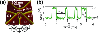
Figure 1: (Color online) (a) Quantum dot with integrated charge read-out used in the experiment. (b) Current through the QPC as a function of time, showing a few electrons tunneling into and out off the dot. The arrows mark the steps corresponding to an electron entering the dot.

The QD used in the experiment is shown in Fig. 1(a). The structure was fabricated using scanning probe lithography Fuhrer et al. (2002) on a $\mathrm{GaAs/Al_{0.3}Ga_{0.7}As}$ heterostructure with a two-dimensional electron gas (2DEG) 34 nm below the surface (electron density $4.5\times 10^{-15}~{}\mathrm{m}^{-2}$, mobility $25~{}\mathrm{m}^{2}/\mathrm{Vs}$). The sample consists of a QD [dotted circle in Fig. 1(a)] and a nearby QPC. We estimate from the geometry and the characteristic energy scales that the dot contains about $30$ electrons. The gates $G1$ and $G2$ were used to tune the tunnel barriers connecting the dot to source and drain leads, while the $P$ gate was used to tune the conductance of the QPC to a regime where the sensitivity to changes in the dot charge is maximal. For our setup, the best sensitivity was reached when the QPC conductance ($G_{QPC}$) was tuned below the first conductance plateau, with $G_{QPC}\sim 0.25\,e^{2}/h$. The conductance was measured by applying a voltage over the QPC ($V_{\mathrm{bias}}=500~{}\mathrm{\mu V}$) and monitoring the current. Since changing the voltages on gates $G1$ and $G2$ also affects the QPC sensitivity, a compensation voltage had to be applied to the $P$-gate in order to keep the QPC in the region of maximum sensitivity whenever the other gates were changed. All measurements where performed in a dilution refrigerator with a base temperature of 60 mK.

When an electron tunnels onto the dot, the conductance through the QPC is reduced due to the electrostatic coupling between the dot and the QPC. A typical time trace of the QPC current is plotted in Fig. 1(b), showing switching between two levels. The low levels correspond to the configuration where the dot contains one extra electron, while $\tau_{\mathrm{in}}$ and $\tau_{\mathrm{out}}$ specify the time it takes for an electron to tunnel into and out of the dot, respectively. The length of each time trace presented here is 0.5 s.

The bandwidth of the QPC circuit is $\Delta f=30~{}\mathrm{kHz}$, which limits the current we can measure by counting electrons to $I\leq e\Delta f\sim 5~{}\mathrm{fA}$. The bandwidth is similar to what was achieved in measurements on a split-gate defined dot Vandersypen et al. (2004). In our setup, the bandwidth is not limited by low signal-to-noise ratio (S/N), but by the low-pass filter formed by the cable capacitance and the feedback resistor of the IV-converter. From the trace shown in Fig. 1(b), we extract $\mathrm{S/N}\sim 15$. Assuming a flat noise spectrum, we estimate that S/N would allow us to increase the bandwidth by a factor of ten and still get a detectable signal. One possible reason for the high sensitivity of our detector compared to split-gate defined structures is that there are no metallic gates on the surface that shield the electrostatic coupling between the QD and the QPC. However, the sensitivity is also strongly dependent on the exact shape of the confinement potential within the QPC and on how susceptible this potential is to changes in the electrostatical environment. This may vary a lot from sample to sample. For the structure used in this measurement, the QPC showed broad resonances in addition to the standard plateau features. By operating the QPC at the flank of a resonance in the step below the first plateau, we were able to find a regime with good sensitivity. For typical current levels in the QPC (nA), electrons pass the QPC at a rate which is many orders of magnitude higher than the rate for electrons passing the quantum dot (aA). We conclude that back action of the QPC via its shot noise can be neglected for the analysis of the counting statistics Gurvitz (1997).

III Thermal noise with one lead connected to the dot

In the following, we are interested in the number of electrons visiting the dot during a given time interval. We call each visit one event and use the symbol $r_{E}$ to denote the number of events occurring per second. In the low-bias Coulomb blockade regime, the dot can only hold one excess electron. Before a new one can enter, another one has to go out. In this case, we can count the events by detecting the electrons as they enter the dot [marked by vertical arrows in Fig. 1(b)]. Note that by counting events, we do not distinguish between electrons passing through the dot and electrons hopping back and forth between the dot and a single lead.

First, we concentrate on the regime where only one lead is connected to the dot and the electron motion is entirely governed by thermal fluctuations and occupation probabilities. For the data shown in Fig. 1(b), the gates are tuned such that the tunnel barrier between the dot and the drain lead is completely closed, while the source lead is weakly coupled to the dot. With only one lead open and with a temperature and level broadening much lower than the charging energy and single level spacing of the QD, only one QD state is available for tunneling. The probability for an electron to tunnel into or out of the dot during a time interval dt is governed by the relation

$$p_{\mathrm{in/out}}(t)\mathrm{dt}=\Gamma_{\mathrm{in/out}}\mathrm{e}^{-\Gamma_{\mathrm{in/out}}t}\mathrm{dt},$$ (1)

where $\Gamma_{\mathrm{in}}$ and $\Gamma_{\mathrm{out}}$ are the effective rates for tunneling into and out of the dot. Using similar methods as in Ref. Schleser et al. (2004); Gustavsson et al. (2006), we have checked that Eq. 1 is fulfilled when we are in the single-level regime. In the following, we consider the case of a non-degenerate level, as discussed in previous work Schleser et al. (2004). To unambiguously determine the spin configuration of the involved states, measurements as a function of magnetic field would be required. Given the availability of our experimental data we focus our analysis on the extraction of the tunneling rates for a single non-degenerate state. We also assume the tunnel coupling to be independent of energy within the small interval of interest. At the end of this section we discuss how the analysis would change if spin degeneracy is relevant.

The relations between the effective rates and the dot-lead tunnel coupling $\Gamma$ are given by

$$\Gamma_{\mathrm{in}}=\Gamma\,f(\Delta E/k_{B}T),~{}\Gamma_{\mathrm{out}}=\Gamma\,(1-f(\Delta E/k_{B}T)),$$ (2)

where $f(x)$ is the Fermi distribution function, $T$ is the temperature and $\Delta E$ is the energy difference between the Fermi level of the lead and the electrochemical potential of the dot.

The tunneling rates can be determined directly from the measured time traces. Using Eq. 1, we find $\Gamma_{\mathrm{in}}=1/\langle\tau_{\mathrm{in}}\rangle,~{}\Gamma_{\mathrm{out}}=1/\langle\tau_{\mathrm{out}}\rangle$, with a relative accuracy of $\sqrt{2\ln 2/N}$ (see Appendix A). Here, $N$ is the total number of switches occurring during one trace. The relative accuracy is calculated assuming that Eq. 1 is valid. For the trace in Fig. 1(b), we get $\Gamma_{\mathrm{in}}=8.0~{}\mathrm{kHz}$, $\Gamma_{\mathrm{out}}=2.3~{}\mathrm{kHz}$ and $\Gamma=1/\langle\tau_{\mathrm{in}}\rangle+1/\langle\tau_{\mathrm{out}}\rangle=10.3~{}\mathrm{kHz}$, with a relative accuracy of $1.7\%$. It has been shown that the finite bandwidth of the detector leads to a systematic under-estimate of the actual rates. For the rates given here we have compensated for such errors using the methods presented in Ref. Naaman and Aumentado (2006), with a detection rate of $\Gamma_{\mathrm{det}}=100~{}\mathrm{kHz}$.

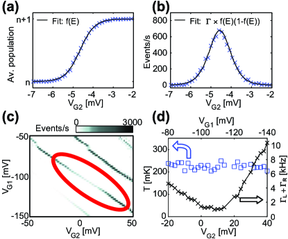
Figure 2: (Color online) (a) Average dot population versus voltage on gate $G2$. The data was fit to a Fermi distribution function with $T=230~{}\mathrm{mK}$. (b) Counts of events per second for the same data as in (a). The data was fit to Eq. (4), giving $\Gamma=2.63~{}\mathrm{kHz}$ and $T=230~{}\mathrm{mK}$. (c) Events per second versus $V_{G1}$ and $V_{G2}$. For low values of $V_{G1}$ and $V_{G2}$, both the source lead and the drain lead are pinched off. For high voltages, the barriers open up so much that the tunneling occurs on a timescale faster than the measurement bandwidth. (d) Temperature (squares) and tunnel coupling (crosses), extracted from data shown within the ellipse in (c). As $V_{G2}$ is increased, $V_{G1}$ is decreased, in order to keep the dot at a constant potential. For low $V_{G2}$, tunneling occurs between the source lead and the dot, for high $V_{G2}$, the electrons tunnel between the drain and the dot. For intermediate gate values, both leads contribute to the tunneling. The electron temperature was found to be the same for both leads, within the accuracy of the data analysis.

Since the dot can only hold one extra electron, we can determine the Fermi function from the average population of excess electrons on the dot

$$f(\Delta E/k_{B}T)=\langle n_{\mathrm{excess}}\rangle=\langle\tau_{\mathrm{out}}\rangle/(\langle\tau_{\mathrm{in}}\rangle+\langle\tau_{\mathrm{out}}\rangle).$$ (3)

The Fermi function can also be found by counting the average number of events occuring per second, $r_{E}$. Assuming sequential tunneling and using Eq. (2), we find for the case with one lead open

$$r_{E}=1/(\langle\tau_{\mathrm{in}}\rangle+\langle\tau_{\mathrm{out}}\rangle)=\Gamma\,f(1-f).$$ (4)

In Fig. 2(a) and (b) we plot the average population and the number of events per second as the gate $G2$ was used to change the electrochemical potential of the dot. The accuracy obtained when determining the Fermi function is $\Delta f=f(1-f)\sqrt{2/N}$ (see Appendix B), giving error bars smaller than the markers used in the figures. The data fits well to the expected relations. By first determining the lever arm between gate $G2$ and the dot from standard Coulomb diamond measurements Kouwenhoven et al. (1997), it was possible to extract the electronic temperature ($T=230~{}\mathrm{mK}$) from the width of the Fermi function. The same temperature was found by checking the width of standard Coulomb blockade current peaks Kouwenhoven et al. (1997), measured when the dot was in a more open regime.

As mentioned earlier, the results shown here are valid only for a non-degenerate level. Taking spin degeneracy into account will modify the value extracted for the tunneling rate $\Gamma$ (see Appendix A), but it will not change the width of the Fermi distribution. The error analysis is performed within the assumption of a non-degenerate level. If spin-degeneracy is taken into account, then some tunneling rates are changed by a factor of two, while the expression for the relative accuracy remains the same as derived before. Further experiments are required to clearly differentiate between spin-degenerate levels and single levels at the Fermi energy. However, the general way how our analysis proceeds is not affected by this.

IV Thermal noise with two leads connected to the dot

In order to perform time-resolved measurements of electron transport through the dot, the tunnel barriers have to be symmetrized so that both give similar tunneling rates. The rates must be kept lower than the bandwidth of the setup, but still high enough to give good statistics. Figure 2(c) shows the number of events per second as a function of the two gates $V_{G1}$ and $V_{G2}$. In the upper left corner of the figure, $V_{G1}$ is high and $V_{G2}$ is low, corresponding to the case where the source lead is open and the drain lead is closed. In the bottom right corner, the opposite is true. For the region in between, marked by the ellipse in Fig. 2(c), the data indicates that both leads are weakly coupled to the dot.

The measurement method does not enable us to distinguish whether an electron that tunnels into the dot arrives from the left or from the right lead. Therefore, when both leads are connected to the dot, the rates in Eq. (2) must be adjusted to contain one part for the left lead and one part for the right lead,

$$\Gamma_{\mathrm{in}}=\Gamma^{\mathrm{in}}_{L}+\Gamma^{\mathrm{in}}_{R}=\Gamma_{L}f_{L}+\Gamma_{R}f_{R},$$

$$\Gamma_{\mathrm{out}}=\Gamma^{\mathrm{out}}_{L}+\Gamma^{\mathrm{out}}_{R}=\Gamma_{L}(1-f_{L})+\Gamma_{R}(1-f_{R}).$$ (5)

Here, $f_{L}$ and $f_{R}$ are the Fermi distribution functions of the left and the right lead, respectively. Using Eq. (IV), we calculate the rate of events for the case when both leads are kept open,

$$r_{E}=\frac{[\Gamma_{L}f_{L}+\Gamma_{R}f_{R}][\Gamma_{L}(1-f_{L})+\Gamma_{R}(1-f_{R})]}{\Gamma_{L}+\Gamma_{R}}.$$ (6)

With no bias applied to the dot, the two distributions functions $f_{L}$ and $f_{R}$ are identical except for a possible difference in electronic temperature in the two leads. However, assuming $T_{L}=T_{R}=T$, we have $f_{L}=f_{R}=f$, and Eq. (6) simplifies to $r_{E}=(\Gamma_{L}+\Gamma_{R})\,f(1-f)$. Fitting this expression to curves similar to that shown in Fig. 2(b), we extract the temperature and combined tunneling rate $\Gamma_{L}+\Gamma_{R}$ from the data within the ellipse of Fig. 2(c). The result is presented in Fig. 2(d). The rates and the temperature shown in the graph are due to the combined tunneling through both leads. Still, for low $V_{G2}$ (high $V_{G1}$), the drain lead is pinched off and tunneling occurs mainly between the source lead and the dot. For high $V_{G2}$ (low $V_{G1}$), the source is pinched off and the tunneling is dominated by electrons going between the drain and the dot. The fact that the electronic temperatures extracted from both regimes turn out to be the same within the accuracy of the analysis (T=230 mK) justifies the assumption that $T_{L}=T_{R}$.

V Shot noise at finite bias

Now we apply a finite voltage bias between source and drain leads and measure electron transport through the dot. Figure 3(a) shows the Coulomb blockade diamonds measured by counting events. In this measurement, the gate $G1$ was used as a plunger gate to control the dot electrochemical potential. However, the gate also strongly affects the source tunnel barrier. For low $G1$ voltages, the source lead is closed, giving strong charge fluctuations only when the drain lead is in resonance with the dot [see case I in Fig. 3(a,b)].

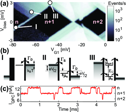
Figure 3: (Color online) (a) Coulomb diamonds, measured by counting events per second. For low values of $V_{G1}$, the source lead is pinched off and tunneling can only occur between the dot and the drain lead. As $V_{G1}$ increases, the source lead opens up and a current can flow through the dot. (b) Diagrams depicting the energy levels of the dot at points I, II and III. In case III, the bias is higher than the charging energy of the dot, meaning that the dot can contain 0, 1 or 2 excess electrons. (c) Time trace taken at point III. The three possible dot populations ($n$, $n+1$ or $n+2$ electrons) are clearly resolvable.

At higher gate voltages, the source lead opens up and a current can flow through the dot. In point II of Fig. 3(a), the dot electrochemical potential $\mu_{n}$ lies within the bias window but far away from the thermal broadening of the Fermi distribution in the leads. The condition can be expressed as

$$|\!\pm\!eV/2-\mu_{n}|\gg k_{B}T,$$ (7)

where the ”+” case refers to the source contact and the ”-” case refers to the drain. Whenever Eq. (7) is fulfilled, electrons can only enter the dot from the source lead and only leave through the drain. In this regime, we measure the current through the dot by counting events. This opens the possibility to use the QD as a very precise current meter for measuring sub-fA currents Bylander et al. (2005). Since the electrons are detected one by one, the noise and higher order correlations of the current can also be experimentally investigated Gustavsson et al. (2006). In this regime we measure the shot noise of the system, which arises because of the discreteness of the charge carriers Blanter and Buttiker (2000). This is in contrast to the results shown in the previous sections, where the fluctuations were due to thermal effects.

When the bias exceeds the dot charging energy, $E_{C}\sim 2.1~{}\mathrm{meV}$, and the electrochemical potentials of the $(n)$ and the $(n+1)$ states are within the bias window [see case III of Fig 3(a,b)], transport processes are allowed where the dot may contain 0, 1 or 2 excess electrons. A time trace measured at point III of Fig. 3(a) is shown in Fig. 3(c). The high sensitivity of the QPC charge detector allows us to measure switching between three different levels, corresponding to $(n)$, $(n+1)$ and $(n+2)$ electrons on the dot. This distinction is not possible in a standard current measurement.

With the condition given by Eq. (7) fulfilled, we know that for positive bias voltage, electrons always enter the dot through the source contact and leave the dot through the drain contact. In this case, we have

$$\Gamma_{S}=\Gamma_{\mathrm{in}}=1/\langle\tau_{\mathrm{in}}\rangle,~{}~{}~{}\Gamma_{D}=\Gamma_{\mathrm{out}}=1/\langle\tau_{\mathrm{out}}\rangle.$$ (8)

Equation (8) can then be used to determine the tunneling rates of an individual state, but only if there are no excited states available within the bias window. If there are excited states available, Eq. (8) will still be valid, however, the calculated $\Gamma_{S}$ and $\Gamma_{D}$ will not be the tunneling rates of a single state but rather the sum of rates from all states contributing to the tunneling process. A further complication with excited states is that there may be equilibrium charge fluctuations between the lead and the excited state, thereby removing the unidirectionality of the electron motion. However, if the relaxation rate of the excited state into the ground state is orders of magnitude faster than the tunneling out rate, the electron in the excited state will have time to relax to the ground state before equilibrium fluctuations can take place.

The separate rates $\Gamma_{\mathrm{in}}$ and $\Gamma_{\mathrm{out}}$ for a close-up of the upper-left region of Fig. 3(a) are plotted in Fig. 4(a) and (b). It is important to note that the requirement of Eq. (7) is met only for the region along and above the dashed lines in the figures. At the lower left end of the dashed lines, the energy levels of the dot are aligned as shown in Fig. 4(c). Going diagonally upward along the lines corresponds to raising the Fermi level of the source lead, while keeping the energy difference between the dot and the drain lead fixed.

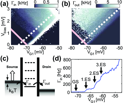
Figure 4: (Color online) (a) and (b): Blow-up of the upper left region of Fig. 3(a), showing the rates for electrons tunneling in (a) and out (b) of the dot, respectively. The solid lines mark the positions where the source lead is lining up with the electrochemical potential of the dot’s ground state. The dashed lines mark the lower edge of the region where condition of Eq. (7) in the text is fulfilled. The color scales are different for the two figures, the rate for tunneling out is around 10 times faster than tunneling in. (c) Diagram depicting the energy levels along the dashed lines in (a) and (b). As the source lead is raised [corresponds to going upward along the dashed lines in (a) and (b)], excited states become available for tunneling. (d) Tunneling rate for electrons entering the dot, measured along the dashed line in (a). With increased gate voltage, excited states become available for transport, giving higher tunneling rates.

Starting at low bias and low voltage on the gate $V_{G1}$, the dot is in the Coulomb blockade regime, and no tunneling is possible. Following the dashed line upwards, the dot ground state becomes available for tunneling at $V_{\mathrm{bias}}=0.3~{}\mathrm{mV}$. The transitions is marked by the solid lines in Fig. 4(a,b). At these low gate voltages, the source tunnel barrier is almost completely pinched off, meaning that the rate for electrons entering the dot is still low [Fig. 4(a)]. Even so, some electrons do enter the dot, as can be seen from the few points of measurements of rates for electrons tunneling out of the dot within the corresponding region of Fig. 4(b).

We now concentrate on the tunneling-in rate in Fig. 4(a). As the source level is further raised, excited states become available for transport. The first excited state (at $V_{\mathrm{bias}}=0.85~{}\mathrm{mV}$ along the dashed line) is more strongly coupled to the lead than the ground state, giving a tunneling rate of $\sim\!70~{}\mathrm{Hz}$ for electrons entering the dot. The large difference in the tunneling-in rate between the ground and the excited state can be understood if the wavefunctions of the ground and excited state have different spatial distributions. If the overlap with the lead wavefunction is larger for the excited state, the tunneling rate will also be larger. Similar differences in tunneling rates have been found between the singlet and triplet states in a two-electron dot Hanson et al. (2005); Ciorga et al. (2002).

By further raising the source level, tunneling can also occur through a second excited state. The measured tunneling-in rate will now be the sum of the rates from both excited states; by subtracting the contribution from the first state, the tunneling-in rate for the second state can be determined. Using this method, we can resolve three excited states, with excitations energies $\varepsilon_{1}=0.55~{}\mathrm{meV}$, $\varepsilon_{2}=1.0~{}\mathrm{meV}$, $\varepsilon_{3}=1.3~{}\mathrm{meV}$ and with tunneling rates $\Gamma_{1}=70~{}\mathrm{Hz}$, $\Gamma_{2}=190~{}\mathrm{Hz}$, $\Gamma_{3}=190~{}\mathrm{Hz}$. The excited states are clearly seen in Fig. 4(d), which is a cut along the dashed diagonal line in Fig. 4(a).

Focusing now on the rates for electrons tunneling out of the dot [Fig. 4(b)], there is a noisy region where the ground state but no excited states are within the bias window ($0.3<V_{\mathrm{bias}}<0.85~{}\mathrm{mV}$ along the dashed line). In this regime, few electrons will enter the dot, meaning that the statistics needed for measuring the rate of electrons leaving the dot is not sufficient. However, for bias voltages higher than the first excited state, the tunneling-out rate remains constant along the dashed line. This is in contrast to the steps seen in the tunneling-in rates, indicating that the rate for tunneling out of the QD does not depend on the state used for tunneling into the QD. Since the individual excited states are expected to have different rates also for tunneling out of the dot, the data is consistent with the interpretation that an electron entering the dot into an excited state will always have time to relax to the ground state before it tunnels out. The rate for tunneling out is $\sim\!6~{}\mathrm{kHz}$, giving an upper bound for the relaxation time of $\sim\!170~{}\mathrm{\mu s}$.

The main relaxation mechanism in quantum dots is thought to be electron-phonon scattering Inoshita and Sakaki (1992). Measurements on few-electron vertical quantum dots have shown relaxation times of $10~{}\mathrm{ns}$ Fujisawa et al. (2002). Recent numerical investigations have shown that the electron-electron interaction in multi-electron dots can lead to reduced relaxation rates Bertoni et al. (2005). Still, the relaxation rate is expected to be considerably faster than the upper limit we give here.

VI Bunching of electrons

So far, we have analyzed data where the tunneling events can be well explained by a rate equation approach with one rate for electrons tunneling into and another rate for electrons leaving the dot. For the trace shown in Fig. 5(a), the behavior is distinctly different. The electrons come in bunches; there are intervals where tunneling occurs on a fast timescale ($>\!10~{}\mathrm{kHz}$), in-between these intervals there are long periods of time ($>\!1~{}\mathrm{ms}$) without any tunneling. The data was taken with a bias applied so that the Fermi level of the source lead is lining up with the electrochemical potential of the dot, while the drain lead is far below the electrochemical potential of the dot, thus prohibiting electrons from entering the dot from the drain lead. The voltage on gate $V_{G1}$ was set to $34~{}\mathrm{mV}$, which is outside the range of the Coulomb diamonds presented in Fig. 3(a). Since the QPC current is at the high level during the intervals without tunneling, the dot contains one electron less when the fast tunneling is blocked.

Figure 5: (Color online) (a) Time trace of the QPC current showing bunching of electrons. (b) Dot states included in the model used to describe the bunching of electrons. The red circles correspond to electron occupation. State $S_{A}$ is the $n$-electron ground state, state $S_{B}$ is an excited $n$-electron state and state $S_{n+1}$ is the ground state when the dot contains $(n+1)$ electrons. (c) Energy diagram for the model. The two dot transitions are both within the thermal broadening of the lead. Electrons enter the dot from the left lead and may leave through either the left or the right lead. (d) Possible transitions between the different states of the model. The rates $\Gamma^{\mathrm{A}}_{\mathrm{in}}$, $\Gamma^{\mathrm{B}}_{\mathrm{in}}$ refer to electrons entering the dot, thus taking the dot from state $S_{A/B}$ to state $S_{n+1}$. The rates $\Gamma^{\mathrm{A}}_{\mathrm{out}}$, $\Gamma^{\mathrm{B}}_{\mathrm{out}}$ describe electrons leaving the dot, giving transitions from state $S_{n+1}$ to $S_{A/B}$. $W_{AB}$ and $W_{BA}$ are the direct transition rates between states $S_{A}$ and $S_{B}$. Finally, the rates $\Gamma^{\mathrm{A}}_{\mathrm{right}}$, $\Gamma^{\mathrm{B}}_{\mathrm{right}}$ refer to electrons leaving the dot through the right lead.

In order to explain the two different timescales, we assume the validity of a model where there are two almost energy-degenerate dot states within the thermal broadening of the distribution in the source lead. Because of Coulomb blockade, the dot may hold one or zero excess electrons. The model includes three possible dot states, shown in Fig. 5(b). State $S_{A}$ is the $n$-electron ground state, state $S_{B}$ is an excited $n$-electron state and state $S_{n+1}$ is the ground state when the dot contains $(n+1)$ electrons. Transitions between the $S_{A}$/$S_{B}$ states and the $S_{n+1}$ state occur whenever an electron tunnels into or out of the dot.

The tunnel coupling between the dot and the lead is given by the overlap of the dot and lead electronic wavefunctions. Since the wavefunctions corresponding to the two states $S_{A}$ and $S_{B}$ may have different spatial distributions, the coupling strength $\Gamma_{A}$ of the transition $S_{A}\Leftrightarrow S_{n+1}$ can vary from the coupling $\Gamma_{B}$ of the $S_{B}\Leftrightarrow S_{n+1}$ transition. The energy levels of the dot and the leads for the configuration where we measure bunching of electrons are shown in Fig. 5(c), while the possible transitions of the model are depicted in Fig. 5(d).

Starting with one excess electron on the dot [state $S_{n+1}$ in Fig. 5(d)], at some point an electron will tunnel out, leaving the dot in either state $S_{A}$ or state $S_{B}$. Assuming $\Gamma_{B}\gg\Gamma_{A}$, it is most likely that the dot will end up in the excited state $S_{B}$. If the tunneling rate $\Gamma_{B}$ is faster than the relaxation process $S_{B}\Rightarrow S_{A}$, an electron from the lead will have time to tunnel onto the dot again and take the dot back to the initial $S_{n+1}$ state. The whole process can then be repeated, leading to the fast tunneling in Fig. 5(a).

However, at some point the dot will end up in state $S_{A}$, either through an electron leaving the dot via the $\Gamma_{A}$ transition, or through relaxation of the $S_{B}$ state. To get out of state $S_{A}$, there must be either a direct transition back to state $S_{B}$, or an electron tunneling into the dot through the $S_{A}\Rightarrow S_{n+1}$ transition. With $\Gamma_{B}\gg\Gamma_{A}$ and assuming $\Gamma_{B}\gg~{}W_{BA}$, both processes are slow compared to the tunneling between the lead and state $S_{B}$. This mechanism will block the fast tunneling and produce the intervals without switching events seen in Fig. 5(a). Similar arguments can be used to show that the blocking mechanism will be possible also if $\Gamma_{B}\ll\Gamma_{A}$.

From the above reasoning, we see that the fast timescale is set by the fast tunneling state, while the slow timescale is determined either by the relaxation process $S_{B}\Rightarrow S_{A}$ or by the slow tunneling rate, depending on which process is the fastest. Either way, it is crucial that the relaxation rate is slower than the fast tunneling rate (in our case $W_{AB}\ll\Gamma_{B}\sim 20~{}\mathrm{kHz}$). We speculate that the slow relaxation rate may be due to different spin configurations of the two states. For a few-electron QD, spin relaxation times of $T_{1}>1~{}\mathrm{ms}$ have been reported Hanson et al. (2005); Elzerman et al. (2004b).

To make quantitative comparisons between the model and the data, we use the framework of full counting statistics (FCS) to investigate how the dot charge fluctuations change as the source lead is swept over a Coulomb resonance. Theoretical investigations of multi-level quantum dots have lead to predictions of electron bunching and super-Poissonian noise Belzig (2005). Following the lines of Refs. Bagrets and Nazarov (2003); Belzig (2005), we first write the master equation for the system,

$$\frac{d}{dt}\left(\begin{array}[]{l}p_{A}\\ p_{B}\\ p_{n+1}\end{array}\right)=M\left(\begin{array}[]{l}p_{A}\\ p_{B}\\ p_{n+1}\end{array}\right),$$ (9)

with $M=$

$$\left(\begin{array}[]{ccc}-\Gamma_{\text{in}}^{A}-W_{BA}&W_{AB}&(\Gamma_{\text{out}}^{A}+\Gamma_{\text{right}}^{A})*e^{i\chi}\\ W_{BA}&-\Gamma_{\text{in}}^{B}-W_{AB}&(\Gamma_{\text{out}}^{B}+\Gamma_{\text{right}}^{B})*e^{i\chi}\\ \Gamma_{\text{in}}^{A}&\Gamma_{\text{in}}^{B}&-\Gamma_{\text{out}}\end{array}\right).$$ (10)

Here $\Gamma_{\text{out}}=(\Gamma_{\text{out}}^{A}+\Gamma_{\text{out}}^{B}+\Gamma_{\text{right}}^{A}+\Gamma_{\text{right}}^{B})$ and $p_{A}$, $p_{B}$ and $p_{n+1}$ are occupation probabilities for states $S_{A}$ and $S_{B}$ and $S_{n+1}$, respectively. The effective tunneling rates are determined by multiplying the tunnel coupling constants for each state with the Fermi distribution of the electrons in the lead,

$$\Gamma_{\text{in/out}}^{A/B}=f[\mp(eV-\mu_{A/B})]\,\Gamma_{A/B}.$$ (11)

The tunneling rates $\Gamma_{\text{right}}^{A}$ and $\Gamma_{\text{right}}^{B}$ are included to account for the possibility for electrons to leave through the right barrier. The Fermi level of the right lead is far below the electrochemical potential of the dot, so that the states in the right lead can be assumed to be unoccupied. Finally, $W_{AB}$ and $W_{BA}$ are the direct transition rates between states $S_{A}$ and $S_{B}$. These rates obey detailed balance,

$$W_{AB}/W_{BA}=\exp\left[(\mu_{A}-\mu_{B})/k_{B}T\right].$$ (12)

The phenomenological relaxation rate between the two states is given as $1/T_{1}=W_{AB}+W_{BA}$.

In Eq. (10), we introduce charge counting by multiplying all entries of $M$ involving an electron leaving the dot with the counting factor $\exp(i\chi)$ Bagrets and Nazarov (2003). We do not distinguish whether the electron leaves the dot through the left or the right lead. In this way we obtain the counting statistics $p_{t_{0}}(N)$, which is the probability for counting $N$ events within the time span $t_{0}$. The distribution describes fluctuations of charge on the dot, which is exactly what is measured by the QPC detector in the experiment. We stress that this distribution is equal to the distribution of current fluctuations only if it can be safely assumed that the electron motion is unidirectional. This is the case if the condition in Eq. (7) is fulfilled, i.e. if the tunneling due to thermal fluctuations is suppressed. Here, we are in a regime where there is a mixture of tunneling due to the applied bias and tunneling due to equilibrium fluctuations. But since the model defined in Eq. (10) is valid regardless of the direction of the electron motion, it can still be used for analyzing the experimental data.

Using the method of Ref. Bagrets and Nazarov (2003), we calculate the lowest eigenvalue $\lambda_{0}(\chi)$ of $M$ and use it to obtain the cumulant generating function (CGF) for $p_{t_{0}}(N)$,

$$S(\chi)=-\lambda_{0}(\chi)t_{0}.$$ (13)

The CGF can then be used to obtain the cumulants of any order using the relation $C_{n}=-(-i\partial_{\chi})^{n}S(\chi)|_{\chi=0}$. In order to compare the theory with the experiment we extract the first three cumulants of $p_{t_{0}}(N)$ from the experimental data. Since we want to compare the data with the predictions given by the CGF of the model, we choose to calculate the cumulants instead of the central moments, as it was done in a previous work Gustavsson et al. (2006). The first cumulant ($C_{1}$) is identical to $\langle N\rangle$, the mean of the distribution, while the second and third cumulants ($C_{2}$, $C_{3}$) coincide with the second and third central moments [$\langle N^{2}\rangle-\langle N\rangle^{2}$ and $(N-\langle N\rangle)^{3}$], giving the variance and the asymmetry of the distribution.

The cumulants were found by taking a trace of length $T=0.5~{}\mathrm{s}$ and splitting it into $m=T/t_{0}$ independent traces. By counting the number of electrons $N$ leaving the dot in each trace and repeating the procedure for all $m$ sub-traces, the distribution function $p_{t_{0}}(N)$ could be experimentally determined. The experimental cumulants were then calculated directly from the measured distribution function Weisstein . The time $t_{0}$ was chosen such that $\langle N\rangle\approx 3$.

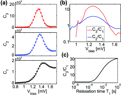
Figure 6: (Color online) (a) First, second and third cumulants of the distribution of charge fluctuations. The markers show values extracted from the experimental data, while the solid lines are calculated from the model given in the text. Fitting parameters are: $\Gamma_{A}=1.6~{}\mathrm{kHz}$, $\Gamma_{B}=20.5~{}\mathrm{kHz}$, $\Gamma_{\text{right}}^{A}=4.6~{}\mathrm{kHz}$, $\Gamma_{\text{right}}^{B}=310~{}\mathrm{Hz}$, $T_{1}=8~{}\mathrm{ms}$ and $\mu_{A}-\mu_{B}=13~{}\mathrm{\mu eV}$. The electronic temperature was 400 mK. (b) Normalized cumulants $C_{3}/C_{1}$ and $C_{2}/C_{1}$ versus bias voltage. The noise is clearly super-Poissonian in the central region of the graph. (c) Calculated maximal value of $C_{3}/C_{1}$ as a function of the relaxation time between the two states. The values are calculated by varying the relaxation time while keeping the other parameters to the values given by the fit shown in (a). The maximum value $C_{3}/C_{1}$ extracted from the experimental data is $15.9$.

Figure 6(a) shows the first three cumulants versus voltage applied to the source lead. The points correspond to experimental data, while the solid lines show the cumulants calculated from the CGF of our model, with fitting parameters $\Gamma_{A}=1.6~{}\mathrm{kHz}$, $\Gamma_{B}=20.5~{}\mathrm{kHz}$, $\Gamma_{\text{right}}^{A}=4.6~{}\mathrm{kHz}$, $\Gamma_{\text{right}}^{B}=310~{}\mathrm{Hz}$, $T_{1}=8~{}\mathrm{ms}$ and $\mu_{A}-\mu_{B}=13~{}\mathrm{\mu eV}$. The electronic temperature in this measurement was 400 mK. The figure shows good agreement between the model and the experimental data.

Figure 6(b) shows the normalized cumulants $C_{2}/C_{1}$ and $C_{3}/C_{1}$ for the experimental data; we notice that both the second and the third cumulants vastly exceed the first cumulant when the Fermi level of the source lead is aligned with the electrochemical potential of the dot ($V_{\mathrm{bias}}=1.3~{}\mathrm{mV}$). The noise is of super-Poissonian nature, as expected from the bunching behavior of the electrons.

When the bias voltage is further increased ($V_{\mathrm{bias}}>1.5~{}\mathrm{mV}$), the source lead is no longer in resonance with the electrochemical potential of the dot and the equilibrium fluctuations between the source and the dot are suppressed. In this regime, the measured charge fluctuations are due to a current flowing through the dot. Electrons enter the dot from the source lead and leave the dot through the drain lead. The blocking mechanism is no longer effective and the transport process will predominantly take place through state $S_{A}$, since the tunnel coupling to the drain lead is stronger for this state ($\Gamma^{A}_{\text{right}}\gg\Gamma^{B}_{\text{right}}$). The transport through the dot can essentially be described by a rate equation, with one rate for electrons entering and another rate for electrons leaving the dot. For such systems, it has been shown that the Coulomb blockade will lead to an increase in correlation between the tunneling electrons compared to a single-barrier structure, giving sub-Poissonian noise Davies et al. (1992); Gustavsson et al. (2006). The effect is seen for $V_{\mathrm{bias}}>1.5~{}\mathrm{mV}$ in Fig 6(b); both the second and third cumulants are reduced compared to the first cumulant.

The value of $T_{1}=8~{}\mathrm{ms}$ obtained from fitting the experimental data is of the same order of magnitude as previously reported values for the spin relaxation time $T_{1}$. We stress that the bunching of electrons and the super-Poissonian noise can only exist if the relaxation time is at least as long as the inverse tunneling time. This is demonstrated in Fig. 6(c), which shows the maximum value obtained for the ratio $C_{3}/C_{1}$ calculated for different $T_{1}$ while keeping the rest of the fitting parameters at the values given in the caption of Fig. 6.

VII Conclusion

In this work, we have shown that a quantum point contact can be used for measuring time-resolved transport through a weakly coupled quantum dot. The detection method allows us to determine the tunneling rates for electrons entering and leaving the dot separately. Comparing the different tunneling rates, information about the excited states and their relaxation times could be extracted. We have shown that the framework of full counting statistics together with time-resolved measurement techniques can be used as a tool for extracting information about electron transport properties of solid state systems.

Appendix A Statistics of tunneling rates

In the single-level regime, the process of an electron tunneling into or out of the dot is described by the rate equation

$$\dot{p}_{\mathrm{in/out}}(t)=-\Gamma_{\mathrm{in/out}}\,p_{\mathrm{in/out}}(t).$$ (14)

Here, $p_{\mathrm{in/out}}(t)$ is the probability density for an electron to tunnel into or out of the dot at a time $t$ after a complementary event. Since the expressions for electrons entering and leaving the dot are the same, we drop the subscripts ($in/out$) and use the notations $p(t)$ and $\Gamma$ to describe either one of the two processes. Solving the differential equation and normalizing the resulting distribution gives

$$p(t)\mathrm{dt}=\Gamma\mathrm{e}^{-\Gamma t}\mathrm{dt}.$$ (15)

Equation 15 is valid assuming non-degenerate states. For the case of spin degeneracy, the rate for tunneling into the dot should be multiplied with a factor of two if both spin states are initially empty.

In the experiment, we measure a time trace containing a sequence of tunneling times $\tau_{k}$, $k=1,2,3,\ldots$ To estimate $\Gamma$ and its relative accuracy from such a sequence, we need to calculate the probability distribution for extracting a certain value $\Gamma$, given a fixed sequence of tunneling times. We start by dividing the time axis into bins of width $\Delta\tau$ and number them with $i=0,1,2,\ldots$ A tunneling event $\tau_{k}$ will be counted in bin $i$ if $i\Delta\tau\leq\tau_{k}<(i+1)\Delta\tau$. Using Eq. (15) and assuming $\Delta\tau\ll 1/\Gamma$, we find that the probability to get a count in bin $i$ for a given value of $\Gamma$ is equal to

$$p(i|\Gamma)=\Gamma\Delta\tau\mathrm{e}^{-\Gamma\Delta\tau\,i}.$$ (16)

A certain sequence $\{i_{n}\}$ is realized with probability

$$p(\{i_{n}\}|\Gamma) = \prod_{n=1}^{N}\Gamma\Delta\tau\mathrm{e}^{-\Gamma\Delta\tau\,i_{n}}=(\Gamma\Delta\tau)^{N}\mathrm{e}^{-\Gamma\Delta\tau\sum_{n=1}^{N}i_{n}}$$ (17)

$$= (\Gamma\Delta\tau)^{N}\mathrm{e}^{-\Gamma\Delta\tau\sum_{i=0}^{\infty}n_{i}i}$$

$$= (\Gamma\Delta\tau)^{N}\mathrm{e}^{-\Gamma\Delta\tau N\langle i\rangle}.$$

Here, $n_{i}$ is the number of times an event falls into bin $i$, $\sum_{i=0}^{\infty}n_{i}=N$ is the total number of events in the trace and $\langle i\rangle=\frac{1}{N}\sum_{i=0}^{\infty}n_{i}i$ is the average of $i$. A certain set of bin occupations $\{n_{i}\}$ can be achieved with many different $\{i_{n}\}$-series, namely $N!/\prod_{i=0}^{\infty}n_{i}!$. Assuming that they all occur with the same probability $p(\{i_{n}\}|\Gamma)$, we find

$$p(\{n_{i}\}|\Gamma)=\frac{N!}{\prod_{i=0}^{\infty}n_{i}!}(\Gamma\Delta\tau)^{N}\mathrm{e}^{-\Gamma\Delta\tau N\langle i\rangle}.$$ (18)

This is our sampling distribution. For an estimate of $\Gamma$ we use Bayes theorem

$$p(\Gamma|\{n_{i}\})=p(\Gamma)\frac{p(\{n_{i}\}|\Gamma)}{p(\{n_{i}\})}.$$ (19)

Because we have no information on the prior probabilities $p(\Gamma)$ and $p(\{n_{i}\})$, the principle of indifference requires them to be constants, giving

$$p(\Gamma|\{n_{i}\})=C\,(\Gamma\Delta\tau)^{N}\mathrm{e}^{-\Gamma\Delta\tau N\langle i\rangle},$$ (20)

where $C$ is constant. Normalization $\int_{0}^{\infty}p(\Gamma|\{n_{i}\})\mathrm{d}\Gamma=1$ leads to

$$p(\Gamma|\{n_{i}\}) = \frac{N^{N}\langle i\rangle^{N+1}\Delta\tau}{N!}(\Gamma\Delta\tau)^{N}\mathrm{e}^{-\Gamma\Delta\tau N\langle i\rangle}$$ (21)

$$= \frac{N^{N}}{N!}\langle\tau\rangle(\Gamma\langle\tau\rangle)^{N}\mathrm{e}^{-N\Gamma\langle\tau\rangle}.$$

The most likely value of $\Gamma$ is therefore $\Gamma^{*}=1/\langle\tau\rangle$. The relative accuracy of this estimate is given by the width of the distribution. Setting $x=\Gamma\langle\tau\rangle$ and evaluating the width at half maximum gives

$$x^{N}\mathrm{e}^{-xN} = \frac{1}{2}\mathrm{e}^{-N}$$

$$\Rightarrow\ln(x) = x-1-\frac{1}{N}\ln(2).$$ (22)

For large $N$ we can expand $\ln(x)$ in a Taylor series around $x=1$. Keeping only the first two terms, it follows

$$\frac{1}{2}(x-1)^{2} = \frac{1}{N}\ln(2)$$

$$\Rightarrow x = 1\pm\sqrt{\frac{2\ln(2)}{N}}.$$ (23)

Thus the relative accuracy is $\Delta\Gamma/\Gamma=\sqrt{2\ln(2)/N}$.

Appendix B Fermi-distribution

With just one lead connected to the QD, we adopt the model $\Gamma_{\mathrm{in}}=D_{n+1}\Gamma f(\Delta E/k_{B}T)$; $\Gamma_{\mathrm{out}}=D_{n}\Gamma[1-f(\Delta E/k_{B}T)]$. Here, $f$ is the Fermi distribution of the lead, $\Gamma$ is the tunnel coupling between the QD and the lead, $D_{n}$ is the spin degeneracy of the state with $n$ electrons on the QD and $\Delta E$ is the energy difference between the electrochemical potential of the QD and the Fermi level of the lead. The tunnel coupling is assumed to be independent of energy within the small interval of interest. Combining the equations gives

$$\frac{\Gamma_{\mathrm{in}}}{\Gamma_{\mathrm{out}}}=\frac{D_{n+1}}{D_{n}}\frac{f}{1-f}.$$ (24)

In the following we will focus on the special case of non-degenerate states, with $D_{n}=D_{n+1}=1$. To determine the Fermi distribution from a sequence of tunneling events, we follow the lines of Appendix A and divide the time axis into bins of width $\Delta\tau$. The bins are labeled with $i=0,1,2,\ldots$, and an event will be counted in bin $i$ if $i\Delta\tau\leq\tau_{\mathrm{in/out}}<(i+1)\Delta\tau$. We collect the tunneling times in two sets of bins, one for electrons tunneling into the dot ($\{n_{i}\}$), and one for electrons leaving the dot ($\{m_{i}\}$). Assuming that the events corresponding to tunneling in and tunneling out are uncorrelated and using the results of Eq. (18), we get

$$p(\{n_{i};m_{i}\}|\Gamma_{\mathrm{in}};\Gamma_{\mathrm{out}})=p(\{n_{i}\}|\Gamma_{\mathrm{in}})p(\{m_{i}\}|\Gamma_{\mathrm{out}})$$

$$\propto(\Gamma_{\mathrm{in}}\Gamma_{\mathrm{out}}\Delta\tau^{2})^{N}\mathrm{e}^{-N(\Gamma_{\mathrm{in}}\langle\tau_{\mathrm{in}}\rangle+\Gamma_{\mathrm{out}}\langle\tau_{\mathrm{out}}\rangle)}.$$ (25)

The principle of indifference gives

$$p(\Gamma_{\mathrm{in}};\Gamma_{\mathrm{out}}|\{n_{i};m_{i}\})\propto$$ (26)

$$~{}~{}~{}(\Gamma_{\mathrm{in}}\Gamma_{\mathrm{out}}\Delta\tau^{2})^{N}\mathrm{e}^{-N(\Gamma_{\mathrm{in}}\langle\tau_{\mathrm{in}}\rangle+\Gamma_{\mathrm{out}}\langle\tau_{\mathrm{out}}\rangle)}.$$

Inserting the result of Eq. (24) leads to

$$p(f;\Gamma_{\mathrm{out}}|\{n_{i};m_{i}\})\propto$$

$$\left(\frac{f}{1-f}\Gamma_{\mathrm{out}}^{2}\Delta\tau^{2}\right)^{N}\mathrm{e}^{-N\Gamma_{\mathrm{out}}\left(\frac{f}{1-f}\langle\tau_{\mathrm{in}}\rangle+\langle\tau_{\mathrm{out}}\rangle\right)}.$$ (27)

Marginalization gives

$$p(f|\{n_{i};m_{i}\}) =\int_{0}^{\infty}p(f;\Gamma_{\mathrm{out}}|\{n_{i};m_{i}\})\mathrm{d}\Gamma_{\mathrm{out}}\propto$$ (28)

$$\frac{\left(\frac{f}{1-f}\right)^{N}(2N+1)!}{\left[\left(\frac{f}{1-f}\langle\tau_{\mathrm{in}}\rangle+\langle\tau_{\mathrm{out}}\rangle\right)N\right]^{2N+1}}.$$

The distribution has a maximum for $\frac{f}{1-f}=\frac{\langle\tau_{\mathrm{out}}\rangle}{\langle\tau_{\mathrm{in}}\rangle}\frac{N}{N+1}.$ In the limit of $N\rightarrow\infty$, the most likely $f$ is given by

$$f=\frac{\langle\tau_{\mathrm{out}}\rangle}{\langle\tau_{\mathrm{in}}\rangle+\langle\tau_{\mathrm{out}}\rangle}.$$ (29)

We find the width of $p(f|\{n_{i};m_{i}\})$ by approximating it around its maximum by a Gaussian. The result is

$$\sigma=f(1-f)\sqrt{2/N}.$$ (30)

References

- Blanter and Buttiker (2000) Y. M. Blanter and M. Buttiker, Physics Reports 336, 1 (2000).
- Levitov et al. (1996) L. S. Levitov, H. W. Lee, and G. B. Lesovik, J. Math. Phys. 37, 4845 (1996).
- Blanter (2005) Y. M. Blanter (2005), cond-mat/0511478.
- Davies et al. (1992) J. H. Davies, P. Hyldgaard, S. Hershfield, and J. W. Wilkins, Phys. Rev. B 46, 9620 (1992).
- Sukhorukov et al. (2001) E. V. Sukhorukov, G. Burkard, and D. Loss, Phys. Rev. B 63, 125315 (2001).
- Cottet et al. (2004) A. Cottet, W. Belzig, and C. Bruder, Phys. Rev. B 70, 115315 (2004).
- Belzig (2005) W. Belzig, Phys. Rev. B 71, 161301(R) (2005).
- Onac et al. (2006) E. Onac, F. Balestro, B. Trauzettel, C. F. J. Lodewijk, and L. P. Kouwenhoven, Phys. Rev. Lett. 96, 026803 (2006).
- Loss and Sukhorukov (2000) D. Loss and E. V. Sukhorukov, Phys. Rev. Lett. 84, 1035 (2000).
- Saraga and Loss (2003) D. S. Saraga and D. Loss, Phys. Rev. Lett. 90, 166803 (2003).
- Lu et al. (2003) W. Lu, Z. Ji, L. Pfeiffer, K. W. West, and A. J. Rimberg, Nature 423, 422 (2003).
- Fujisawa et al. (2004) T. Fujisawa, T. Hayashi, Y. Hirayama, H. D. Cheong, and Y. H. Jeong, Appl. Phys. Lett. 84, 2343 (2004).
- Bylander et al. (2005) J. Bylander, T. Duty, and P. Delsing, Nature 434, 361 (2005).
- Gustavsson et al. (2006) S. Gustavsson, R. Leturcq, B. Simovic, R. Schleser, T. Ihn, P. Studerus, K. Ensslin, D. C. Driscoll, and A. C. Gossard, Phys. Rev. Lett. 96, 076605 (2006).
- Field et al. (1993) M. Field, C. G. Smith, M. Pepper, D. A. Ritchie, J. E. F. Frost, G. A. C. Jones, and D. G. Hasko, Phys. Rev. Lett. 70, 1311 (1993).
- Schleser et al. (2004) R. Schleser, E. Ruh, T. Ihn, K. Ensslin, D. C. Driscoll, and A. C. Gossard, Appl. Phys. Lett. 85, 2005 (2004).
- Elzerman et al. (2004a) J. M. Elzerman, R. Hanson, L. H. Willems van Beveren, L. M. K. Vandersypen, and L. P. Kouwenhoven, Appl. Phys. Lett. 84, 4617 (2004a).
- Fuhrer et al. (2002) A. Fuhrer, A. Dorn, S. Lüscher, T. Heinzel, K. Ensslin, W. Wegscheider, and M. Bichler, Superl. and Microstruc. 31, 19 (2002).
- Vandersypen et al. (2004) L. M. K. Vandersypen, J. M. Elzerman, R. N. Schouten, L. H. Willems van Beveren, R. Hanson, and L. P. Kouwenhoven, Appl. Phys. Lett. 85, 4394 (2004).
- Gurvitz (1997) S. A. Gurvitz, Phys. Rev. B 56, 15215 (1997).
- Naaman and Aumentado (2006) O. Naaman and J. Aumentado, Phys. Rev. Lett. 96, 100201 (2006).
- Kouwenhoven et al. (1997) L. P. Kouwenhoven, C. M. Marcus, P. M. McEuen, S. Tarucha, R. M. Westervelt, and N. S. Wingreen, in Mesoscopic Electron Transport, edited by L. L. Sohn, L. P. Kouwenhoven, and G. Schön (Kluwer, Dordrecht, 1997), NATO ASI Ser. E 345, pp. 105–214.
- Hanson et al. (2005) R. Hanson, L. H. Willems van Beveren, I. Wink, J. M. Elzerman, W. J. M. Naber, F. H. L. Koppens, L. P. Kouwenhoven, and L. M. K. Vandersypen, Phys. Rev. Lett. 94, 196802 (2005).
- Ciorga et al. (2002) M. Ciorga, A. Wensauer, M. Pioro-Ladriere, M. Korkusinski, J. Kyriakidis, A. S. Sachrajda, and P. Hawrylak, Phys. Rev. Lett. 88, 256804 (2002).
- Inoshita and Sakaki (1992) T. Inoshita and H. Sakaki, Phys. Rev. B 46, 7260 (1992).
- Fujisawa et al. (2002) T. Fujisawa, D. G. Austing, Y. Tokura, Y. Hirayama, and S. Tarucha, Nature 419, 278 (2002).
- Bertoni et al. (2005) A. Bertoni, M. Rontani, G. Goldoni, and E. Molinari, Phys. Rev. Lett. 95, 066806 (2005).
- Elzerman et al. (2004b) J. M. Elzerman, R. Hanson, L. H. Willems van Beveren, B. Witkamp, L. M. K. Vandersypen, and L. P. Kouwenhoven, Nature 430, 431 (2004b).
- Bagrets and Nazarov (2003) D. A. Bagrets and Y. V. Nazarov, Phys. Rev. B 67, 085316 (2003).
- (30) E. W. Weisstein, ”Cumulant.” From MathWorld - A Wolfram Web Resource. http://mathworld.wolfram.com/Cumulant.html.