Stabilisation of the lattice-Boltzmann method
using the Ehrenfests’ coarse-graining
Abstract
The lattice-Boltzmann method (LBM) and its variants have emerged as promising, computationally efficient and increasingly popular numerical methods for modelling complex fluid flow. However, it is acknowledged that the method can demonstrate numerical instabilities, e.g., in the vicinity of shocks. We propose a simple and novel technique to stabilise the lattice-Boltzmann method by monitoring the difference between microscopic and macroscopic entropy. Populations are returned to their equilibrium states if a threshold value is exceeded. We coin the name Ehrenfests’ steps for this procedure in homage to the vehicle that we use to introduce the procedure, namely, the Ehrenfests’ idea of coarse-graining.
pacs:
47.11.-j; 04.60.Nc; 47.40.-x; 65.40.GrI Introduction
The lattice-Boltzmann method (LBM) provides an alternative to the orthodox approach to computational fluid dynamics, in which the starting point is always a discretization of the Navier–Stokes equations. The method, which is fundamentally based on Boltzmann’s kinetic transport equation, instead describes a fluid by a number of interacting populations of particles moving and colliding on a fixed lattice. With the advent of the introduction of a diagonal collision integral with single-time relaxation to local equilibrium, the method becomes tantalisingly simple and efficient.
In recent years, the LBM has enjoyed much applied success modelling various flows of genuine engineering interest (see e.g., Succi (2001) and the references therein). However, when populations are far from equilibrium, such as is the case in the vicinity of shocks, the LBM exhibits numerical instability. Often, numerical instability in the LBM is attributed to the absence of a positivity constraint on the populations. Recent development of the entropic LBM (ELBM) Ansumali and Karlin (2000); Boghosian et al. (2001); Ansumali and Karlin (2002) are attempts to improve stability properties through compliance with a discrete entropy -theorem. Although such techniques should, conceivably, reduce the magnitude of spurious oscillations, one should perhaps not be disappointed to find that such numerical instabilities are not removed entirely.
In this paper we suggest an alternative and versatile approach. The idea is simply stated: we propose a LBM in which the difference between microscopic and macroscopic entropy is monitored in the simulation, and populations are returned to their equilibrium states if a threshold value is exceeded. This technique is appealing because dissipation is introduced in a controlled, targeted and illiberal manner. Furthermore, we stress that equilibration itself will leave macroscopic entropy completely unchanged.
We coin the name Ehrenfests’ steps for this procedure because we feel that the technique is most clearly understood if introduced using the Ehrenfests’ coarse-graining idea Ehrenfest and Ehrenfest (1990).
This report is organised as follows. In Section II the LBM is recalled. In Section III we recall the basic theory required to discuss the Ehrenfests’ coarse-graining and introduce Ehrenfests’ steps. The reader is directed to Gorban (2006) for a more comprehensive review of coarse-graining. Finally, we present the results of a shock tube numerical experiment which compares various LBMs.
II Lattice-Boltzmann method
The Boltzmann kinetic transport equation is the following time evolution equation for one-particle distribution functions :
The collision integral, , describes the interactions of the populations . The lattice-Boltzmann approach drastically simplifies this model by stipulating that populations can only move with a finite number of velocities :
| (1) |
where is the one-particle distribution function associated with motion in the th direction. For example, in one-dimension, one might consider three velocities , for some .
The model is further simplified by specifying the collision integral as the Bhatnager–Gross–Krook (BGK) operator Bhatnager et al. (1954): . We make this assumption for the remainder of the paper. Now, (1) describes free-flight dynamics together with relaxation to local equilibria, , in time proportional to .
The discrete velocities and local equilibrium states can all be mindfully chosen so that the Navier–Stokes equations are recovered by the lattice-Boltzmann equation (1), subject to ceratin conservation laws, in the large time-scale, , limit via a Chapman–Enskog procedure Succi (2001). Here, the macroscopic fluid density and momentum are the zeroth- and first-order hydrodynamic moments of the populations respectively. The rate of dissipation introduced by the model is proportional to .
The local equilibrium states can be found by maximising a local entropy functional subject to the constraints of conservation of mass and momentum.
There are numerous ways to discretize (1) and obtain a numerical method. We prefer the following, second-order accurate in time, lattice-based LBGK scheme Succi (2001):
| (2) |
with . Here, the discrete velocities are associated with an underlying spatial lattice and . Populations live on this lattice, propagate to neighbouring lattice sites with their corresponding discrete velocities and are updated via (2). The parameter controls the viscosity in the model, with corresponding to the zero-viscosity limit.
III The Ehrenfests’ coarse-graining
To introduce the Ehrenfests’ coarse-graining idea Ehrenfest and Ehrenfest (1990) we use a formal kinetic equation
| (3) |
together with a strictly concave entropy functional . We tacitly assume that entropy does not decrease with time: . For our purposes, we are always interested in the example of the lattice-Boltzmann equation (1) with associated entropy functional which defines the local equilibrium states.
The Ehrenfests’ idea was to supplement the mechanical motion from (3) with periodic averaging in cells to produce piecewise constant, or coarse-grained, densities. This operation necessitates entropy production.
We wish to allow a generalisation of the Ehrenfests’ coarse-graining whereby averaging in cells is replaced with some other partial equilibration procedure. Specifically, we assume we have some linear operator which transforms a microscopic description of the system into a macroscopic description . For our example, the macroscopic description is that provided by the usual hydrodynamic moments. Now, given a macroscopic description, , we consider the solution of the optimisation problem
| (4) |
Averaging in cells is a particular example of this entropy maximisation problem for the Boltzmann–Gibbs–Shannon (BGS) entropy functional , where the integration is taken over the whole of phase space.
We will refer to as the quasi-equilibrium distribution. The quasi-equilibrium manifold is the set of quasi-equilibrium distributions parameterised by the macroscopic variables .
III.1 The Ehrenfests’ chain and entropic involution
Entropy maximisation leads naturally to an evolution equation for the macroscopic description. The so-called quasi-equilibrium approximation to (3) is an equation for the evolution of :
| (5) |
For our example, the quasi-equilibrium distributions are precisely the local equilibria and (5) coincides with the compressible Euler equations Gorban et al. (2001).
Now, one can envisage constructing various coarse-graining chains which provide stepwise approximation to the macroscopic equations (5).
Let be the phase flow for the kinetic equation (3). Let be a fixed coarse-graining time and suppose we have an initial quasi-equilibrium distribution . The Ehrenfests’ chain is the sequence of quasi-equilibrium distributions , where .
Entropy increases in the Ehrenfests’ chain. The entropy gain in a link in the chain is made up from two parts: the entropy gain from the mechanical motion (from to ) and the gain from the equilibration (from to ). Consequently, conservative systems become dissipative and dissipative systems more so. The gain in macroscopic entropy in a particular link is given by the expression . Note that there is zero gain in macroscopic entropy from the equilibration part.
The Ehrenfests’ chain provides a stepwise approximation to a solution of some coarse-grained macroscopic equations via , . For our example, these equations are the compressible Navier–Stokes equations Gorban et al. (2001). However, this chain is computationally prohibitive because the rate of introduced dissipation is proportional to . The Ehrenfests’ chain corresponds to the following LBM:
which we recognise as a forward Euler discretization of (1).
Another possibility is to construct a chain as follows. As already noted, the dissipative term introduced by the Ehrenfests’ chain depends linearly on . Therefore, there is symmetry between forward and backward motion in time starting from any quasi-equilibrium initial condition. It is precisely this principle that enables one to construct chains with zero macroscopic entropy production. Each subsequent link in the chain is constructed using entropic involution.
To make such a chain useful, the user is at liberty to add a required amount of dissipation by shifting the involuted point in the direction of the quasi-equilibrium state, with some entropy increase. Of course, this shift leaves macroscopic entropy unchanged. This chain corresponds to the ELBM that we have eluded to in the introduction:
| (6) |
with . The number is chosen so that a constant entropy condition is satisfied. This, in itself, provides a positivity constraint on the populations.
If the entropic involution operator is partially linearised so that subsequent links are constructed with the use of reflections in the quasi-equilibrium manifold, rather than inversions, then the corresponding LBM is precisely LBGK (2).
III.2 Ehrenfests’ steps
We can now state the main idea of the paper. We propose to create a new chain. This chain begins and proceeds, for the bulk of time, as the either the entropic involution chain or its linearised version, as described in the previous subsection. However, the difference between microscopic and macroscopic entropy is monitored throughout the simulation, by which we mean the quantities
A threshold value is set and an alarm is triggered if exceeded. The alarm simply signals that a link from the Ehrenfests’ chain — an Ehrenfests’ step — be used in place of a regular link of the primary chain at this point. Links in the chain which are intolerably far from their quasi-equilibrium states are merely returned to their equilibrium. The result is a chain which provides additional dissipation only where it is anticipated to be required.
Coupling the entropic involution chain with Ehrenfests’ steps will, in general, no longer constitute a chain with zero macroscopic entropy production. Indeed, in a chain of length the total macroscopic entropy gain is given by the expression , where is the set of indices corresponding to the Ehrenfests’ steps.
IV Numerical experiment
To conclude this report, we perform a one-dimensional numerical experiment to demonstrate the performance of the proposed LBM corresponding to a chain with Ehrenfests’ steps. The implementation is as follows. If , for some given tolerance then we accept an Ehrenfests’ step. The resulting LBM is as follows:
| (7) |
We have selected LBGK (2) as the primary chain and we will henceforth refer to this LBM as LBGK-ES.
The method LBGK-ES, as described, is a second-order accurate in time scheme with first-order degradation in regions where Ehrenfests’ steps are employed. However, as is often found, when the thickness of such regions is of the order of the lattice spacing, the method remains second-order everywhere.
For contrast we are interested in comparing LBGK-ES with LBGK (1) and ELBM (6) (as described in Ansumali and Karlin (2002)). In all of our simulations we select the three-velocity model mentioned in the introduction and a uniformly spaced lattice. Further, we always choose and . The coefficient , which controls the viscosity in the model, is fixed at , which is close to the zero viscosity limit. In each case the entropy is , with Karlin et al. (1999), where , and denote the static, left-moving and right-moving populations respectively. For this entropy, the local equilibria are available analytically for the three-velocity model. They are given by the expressions
For LBGK-ES we fix the tolerance, , to either or .
As already mentioned, for ELBM, there is a parameter, , which is chosen to satisfy a constant entropy condition. This involves finding the nontrivial root of the equation
| (8) |
Inaccuracy in the solution of this equation can introduce artificial viscosity. To solve (8) numerically we employ a robust routine based on bisection. The root is solved to an accuracy of . Furthermore, we always ensure that the returned value of does not lead to an entropy decrease. So that our results can be faithfully reproduced, we stipulate that we will consider two possibilities if no nontrivial root of (8) exists. We either elect to select or we select the positivity bound , with . For fairness, since both of these procedures introduce diffusivity into ELBM, we consider analogous procedures for LBGK too, i.e., we elect to select either or if a populations is predicted to become negative.
IV.1 Shock tube results
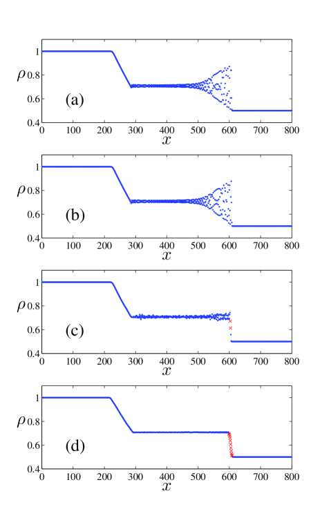
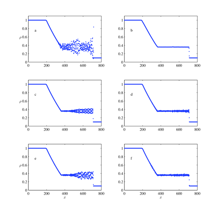
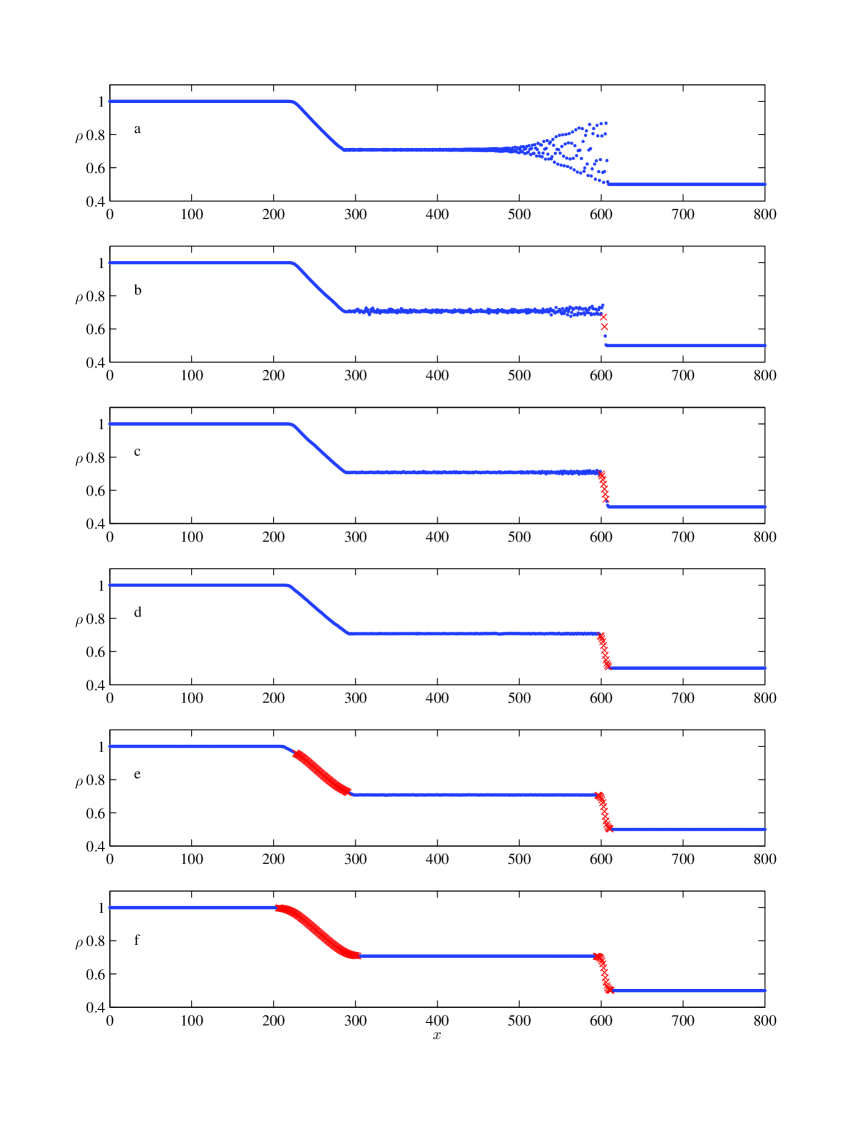
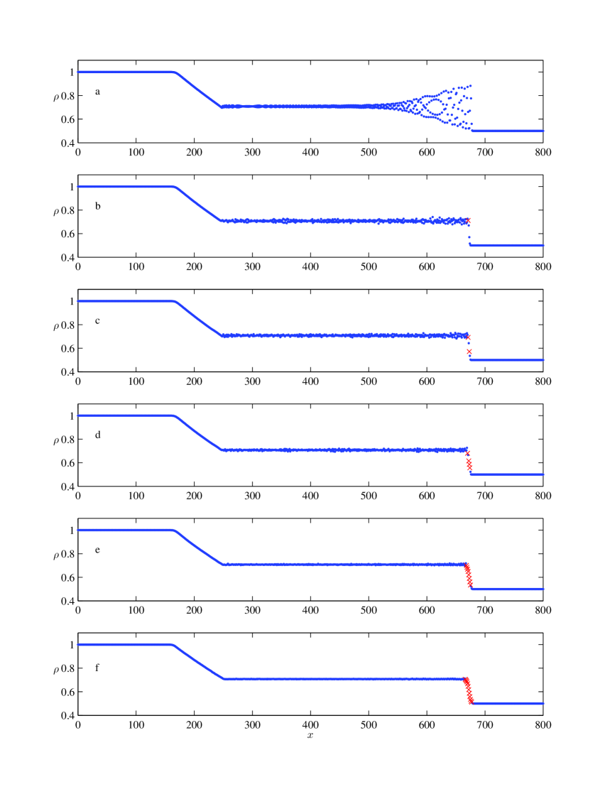
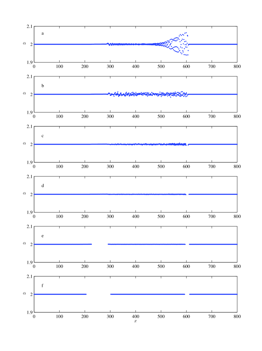
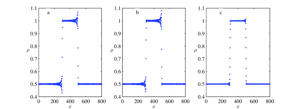
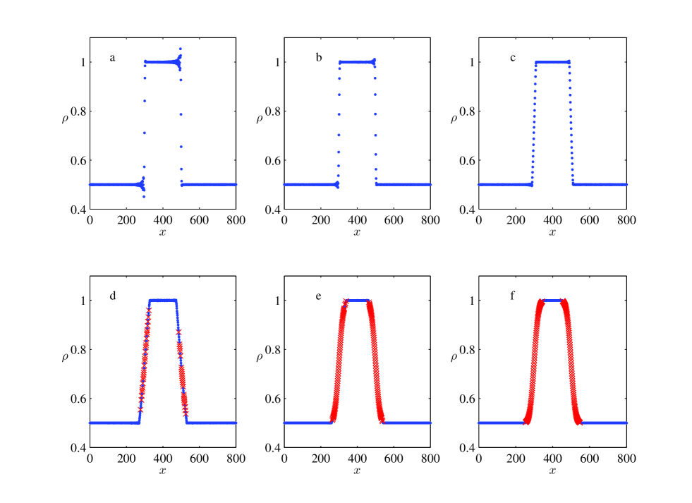
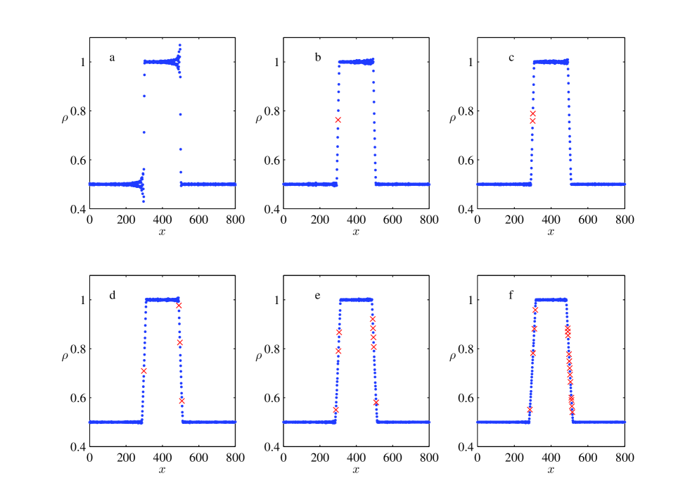
The one-dimensional shock tube for a compressible isothermal fluid is a standard benchmark test for hydrodynamic codes. Our computational domain will be the interval and we discretize this interval with uniformly spaced lattice sites. We choose the initial density ratio as . Initially, for we set else we set .
We observe that, of all the LBMs considered in the experiment, only the method which includes Ehrenfests’ steps is capable of suppressing spurious post-shock oscillations (Fig. 1).
The code used to produce the simulations in this section is freely available by making contact with the corresponding author.
Conclusion
Ehrenfests’ steps introduce additional dissipation locally, on the base of point-wise analysis of non-equilibrium entropy. They admit a huge variety of generalisations: incomplete Ehrenfests’ steps, partial involution, etc. Gorban (2006). In order to preserve the second-order of LBM accuracy it is worthwhile to perform Ehrenfests’ steps on only a small share of sites (the number of sites should be , where is the number of sites, is the macroscopic characteristic length and is the lattice step) with highest . Numerical experiments show that even small shares of such steps drastically improve stability. More tests are presented in Brownlee et al. (2006).
Acknowledgements.
The first author is grateful for a series of invaluable and encouraging discussions with Ilya Karlin and Shyam Chikatamarla. This work is supported by Engineering and Physical Sciences Research Council (EPSRC) grant number GR/S95572/01.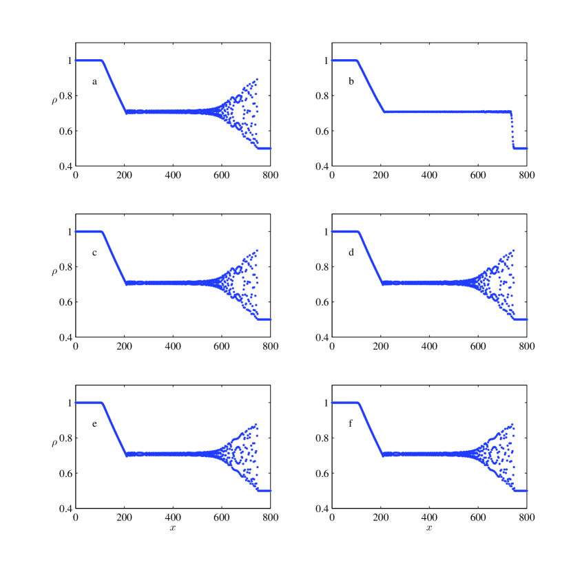
References
- Succi (2001) S. Succi, The lattice Boltzmann equation for fluid dynamics and beyond (OUP, New York, 2001).
- Ansumali and Karlin (2000) S. Ansumali and I. V. Karlin, Phys. Rev. E. 62, 7999 (2000).
- Boghosian et al. (2001) B. M. Boghosian, J. Yepez, P. V. Coveney, and A. J. Wager, R. Soc. Lond. Proc. Ser. A Math. Phys. Eng. Sci. 457, 717 (2001), ISSN 1364-5021.
- Ansumali and Karlin (2002) S. Ansumali and I. V. Karlin, J. Stat. Phys. 107, 291 (2002).
- Ehrenfest and Ehrenfest (1990) P. Ehrenfest and T. Ehrenfest, The conceptual foundations of the statistical approach in mechanics (Dover, New York, 1990).
- Gorban (2006) A. N. Gorban, arXiv cond-mat/0602024 (2006).
- Bhatnager et al. (1954) P. L. Bhatnager, E. P. Gross, and M. Krook, Phys. Rev. 94, 511 (1954).
- Gorban et al. (2001) A. N. Gorban, I. V. Karlin, H. C. Öttinger, and L. L. Tatarinova, Phys. Rev. E. 63, 066124 (2001).
- Karlin et al. (1999) I. V. Karlin, A. Ferrante, and H. C. Öttinger, Europhys. Lett. 47, 182 (1999).
- Brownlee et al. (2006) R. A. Brownlee, A. N. Gorban, and J. Levesley, arXiv cond-mat/0605359 (2006).