Ballistic transport in ferromagnet–superconductor–ferromagnet trilayers with arbitrary orientation of magnetizations

Abstract

Transport phenomena in clean ferromagnet–superconductor–ferromagnet (FSF) trilayers are studied theoretically for a general case of arbitrary orientation of in-plane magnetizations and interface transparencies. Generalized expressions for scattering probabilities are derived and the differential conductance is computed using solutions of the Bogoliubov–de Gennes equation. We focus on size and coherence effects that characterize ballistic transport, in particular on the subgap transmission and geometrical oscillations of the conductance. We find a monotonic dependence of conductance spectra and magnetoresistance on the angle of misorientation of magnetizations as their alignment is changed from parallel to antiparallel. Spin-triplet pair correlations in FSF heterostructures induced by non-collinearity of magnetizations are investigated by solving the Gor’kov equations in the clean limit. Unlike diffusive FSF junctions, where the triplet correlations have a long-range monotonic decay, we show that in clean ferromagnet-superconductor hybrids both singlet and triplet pair correlations induced in the F layers are oscillating and power-law decaying with the distance from the S-F interfaces.

I Introduction

The interplay between ferromagnetism and superconductivity in thin film systems is a phenomenon that attracts considerable interest of researchers for some time already.Buzdin_rev Apart from potential device applications, ferromagnet–superconductor (F–S) hybrid structures can be major tools in the quest for novel superconducting phenomena.Pokrovsky_rev ; BVE_rev Variety of interesting theoretical predictions, such as the existence of $\pi$-state superconductivity in F–S multilayer systems,Bulaevski ; FFLO ; Buzdin82 and characteristic oscillations in the superconducting transition temperature as a function of thickness of ferromagnetic layers,Radovic91 ; Buzdin90 ; Demler ; Tagirov_C ; FCG ; Bagrets have been already confirmed experimentally,Kontos ; Ryazanov ; Jiang ; Lazar ; Garifullin ; Obi while the existence of the spin valve effectTagirov_PRL ; Baladie was more difficult for confirmation than expected.Gu ; PRL2005 Other peculiar phenomena that have been predicted to exist in F–S hybrids with inhomogeneous magnetization – the occurrence of a long-range triplet pairing,F1 ; BVE_PRL ; F2 ; KK ; VBE or the so-called inverse proximity effectBVE_PRB – still wait for experimental realization. Hence, a proper understanding of these effects is a prerequisite for setting up appropriate experimental conditions.

Long-range triplet pairing, in particular, was first predicted as a consequence of proximity of an inhomogeneous ferromagnet to a superconductor.F1 ; BVE_PRL ; F2 ; KK However, it was shown that spin-triplet pair correlations may also arise in layered structures consisting of superconductors and homogeneous ferromagnets with differently oriented magnetizations.VBE ; Kupriyanov The simplest structure of this kind is an FSF system with homogeneous but non-collinear magnetizations of the ferromagnets. In the parallel (P) or the antiparallel (AP) alignment such correlations are absent. It was found that in diffusive junctions triplet correlations have a long-range monotonically decaying component in the ferromagnetic layers.VBE Very recently, effects of these correlations seem to have been observed in half-metallic ferromagnets.Keizer ; Penya ; Eschrig03

In this paper we study a variety of effects that occur due to the interplay of ferromagnetism and superconductivity in clean FSF double junctions. It has been already established for the case of collinear magnetizations that the most significant consequences of quantum interference in such structures are the subgap transmission and the periodic vanishing of the Andreev reflection.BozovicB The annulment of the Andreev reflection occurs at the energies of geometrical resonances, which correspond to the maxima in the density of states. Here, we investigate these phenomena in FSF hybrids with an arbitrary angle between magnetizations. In particular, we address the issue of triplet correlations, and describe its influence on transport properties.

We use solutions of the Bogoliubov–de Gennes equation in the scattering formulation (Section II) to obtain the probabilities of processes that charge carriers undergo and calculate the conductance spectra for arbitrary orientation of magnetizations. Section III illustrates some typical cases. In particular, the conductance spectra of a clean FSF hybrid with a thin superconducting layer (i.e., such that the layer thickness $d_{s}$ is less or of the order of the superconducting coherence length $\xi_{0}=\hbar v_{\rm F}/\pi\Delta_{0}$) are dominated by subgap transport since majority of the charge carriers is transferred directly from one electrode to another without interaction with superconducting condensate.BozovicB ; Yamashita67 On the other hand, situation in the junctions with a thick superconducting layer ($d_{s}\gg\xi_{0}$) is quite the opposite: majority of the carriers form Cooper pairs, thereby increasing the subgap conductance; also, the conductance spectra show pronounced oscillatory behavior above the gap due to interference-generated geometric resonances inside the superconductor. However, we show that no extraordinary effects arise when the relative orientation of magnetizations is between parallel and antiparallel – the spectra for intermediary angles simply fall in between those for P and AP alignment. The obtained results allow us to infer some general conclusions about the nature of ballistic transport properties of FSF hybrids, which we illustrate on the example of dependence of magnetoresistance on voltage and S-layer thickness (Section IV). In Section V we address the problem of spin-triplet pair correlations when magnetizations are non-collinear. By solving the Gor’kov equations in the clean limit, we show that both triplet and singlet superconducting correlations induced in ferromagnets are oscillatory functions of distance from S-F interfaces, with a power law decay. This result is consistent with obtained monotonicity of transport properties as the angle of relative orientation of magnetizations is varied.

II The model

We consider an FSF double junction consisting of a clean superconducting (S) layer of thickness $d_{s}$, connected to clean ferromagnetic layers (F) of thickness $d_{f}$ via thin insulating interfaces (I), Fig. 1. To describe the ferromagnets we use the Stoner model for inhomogeneous exchange field ${\bf h}({\bf r})$ lying in $y$-$z$ plane, parallel to the layers. The exchange field has, in general, different orientations in the left and right ferromagnet, which (without loss of generality) we take to be symmetric with respect to the $z$-axis

$${\bf h}({\bf r})=h_{0}\left(0,\pm\sin(\alpha/2),\cos(\alpha/2)\right),$$ (1)

${\rm for}~{}|x|>d_{s}/2.$ The case $\alpha=0$ ($\alpha=\pi$) then corresponds to the P (AP) alignment of magnetizations.

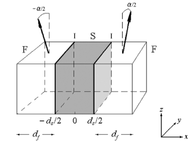
Figure 1: A schematic of an FSF junction with magnetization vectors lying in $y$-$z$ planes, at angles $\pm\alpha/2$ with the $z$ axis. The $x$-axis is perpendicular to the layer interfaces. The strength of insulating barriers (I) at the interfaces is measured by a dimensionless parameter $Z=2W_{0}/\hbar v_{\rm F}$.

Quasiparticle propagation is described by the Bogoliubov–de Gennes equation

$$\check{\cal{H}}\Psi({\bf r})=E\Psi({\bf r})$$ (2)

for the four-vectors $\Psi({\bf r})\equiv\left(u_{\uparrow}({\bf r})~{}u_{\downarrow}({\bf r})~{}v_{\downarrow}({\bf r})~{}v_{\uparrow}({\bf r})\right)^{\rm T}$, where the Hamiltonian can be written in the compact form as

$$\check{\cal{H}}=\widehat{\tau}_{3}\otimes\left(\widehat{H}_{0}({\bf r})-{\bf h}({\bf r})\cdot\widehat{\bm{\sigma}}\right)+\widehat{\Delta}({\bf r})\otimes\widehat{\bm{1}}.$$ (3)

Here, $\widehat{\tau}_{i}$ and $\widehat{\sigma}_{i}$ are the Pauli matrices in orbital and spin space, respectively, $\widehat{\bm{1}}$ is $2\times 2$ unity matrix,

$$\widehat{H}_{0}({\bf r})=\left(\begin{array}[]{cc}H_{0}({\bf r})&0\\ 0&H^{\ast}_{0}({\bf r})\end{array}\right),$$ (4)

$H_{0}({\bf r})=-\hbar^{2}\nabla^{2}/2m+W({\bf r})+U({\bf r})-\mu$ being the one-particle Hamiltonian, $U({\bf r})$ and $\mu$ are the Hartree and the chemical potential, respectively, while $E$ is the energy with respect to $\mu$. The interface potential is modeled symmetrically by $W({\bf r})=W_{0}\left[\delta(x+d_{s}/2)+\delta(x-d_{s}/2)\right]$, where $\delta$ is the Dirac delta-function. The matrix $\widehat{\Delta}$ is given by

$$\widehat{\Delta}({\bf r})=\left(\begin{array}[]{cc}0&\Delta({\bf r})\\ \Delta^{\ast}({\bf r})&0\end{array}\right),$$ (5)

where $\Delta({\bf r})$ is the pair potential. We will not consider the case of a ferromagnetic superconductor,Eschrig ; Eschrig05 ; Dong05 ; Marion and henceforth we take ${\bf h}({\bf r})=0$ outside the ferromagnets and $\Delta({\bf r})=0$ outside the superconductor. Since there is only one S layer in the system, without loss of generality we can choose $\Delta$ to be real. The electron effective mass $m$ is assumed to be the same throughout the junction. For simplicity, the Fermi energy of the superconductor and the mean Fermi energy of the ferromagnets are assumed to be the same, $E_{\rm F}$. The model could be straightforwardly generalized to the case of a Fermi velocity mismatch between the layers (see, e.g. Ref. BozovicB, ).

Wave-vector components have to be normalized by using the condition for canonical transformation, which after integration over the volume of the S layer reads

$$\int{\rm d}^{3}{\bf r}\left[|u_{\sigma}({\bf r})|^{2}+|v_{\bar{\sigma}}({\bf r})|^{2}\right]=1.$$ (6)

Here, $\sigma$ denotes the spin orientation, ($\sigma=\uparrow,\downarrow$) and $\bar{\sigma}$ is opposite to $\sigma$. As the exchange field removes spin degeneracy, a spin-generalized gap equation has to be used.BozovicEPL Using the condition for the singlet pairing in the superconductor,

$$\sum_{{\bf q}}\left[u_{\uparrow}({\bf r})v^{\ast}_{\downarrow}({\bf r})-u_{\downarrow}({\bf r})v^{\ast}_{\uparrow}({\bf r})\right]=0,$$ (7)

for $|x|\leq d_{s}/2$, the gap equation can be written in familiar form

$$\Delta({\bf r})=V({\bf r})\sum_{\bf q}\left[u_{\uparrow}({\bf r})v^{\ast}_{\downarrow}({\bf r})+u_{\downarrow}({\bf r})v^{\ast}_{\uparrow}({\bf r})\right]\tanh\left(\frac{E}{k_{\rm B}T}\right).$$ (8)

In Eqs. (7) and (8) the summation is performed over wave vectors in the superconductor ${\bf q}$, taking into account the dispersion relation between ${\bf q}$ and $E$. Also, we assume for simplicity that the pairing interaction potential $V({\bf r})=V=const.$ inside the superconductor.

The parallel component of the wave vector, ${\bf k}_{||,\sigma}$, is conserved due to translational invariance of the junction in directions perpendicular to the $x$-axis, but differs for the two spin orientations. Consequently, the wave function can be written in the form

$$\Psi({\bf r})=\left(\begin{array}[]{c}\widetilde{u}_{\uparrow}(x)e^{i{\bf k}_{||,\uparrow}\cdot{\bf r}}\\ \widetilde{u}_{\downarrow}(x)e^{i{\bf k}_{||,\downarrow}\cdot{\bf r}}\\ \widetilde{v}_{\downarrow}(x)e^{i{\bf k}_{||,\uparrow}\cdot{\bf r}}\\ \widetilde{v}_{\uparrow}(x)e^{i{\bf k}_{||,\downarrow}\cdot{\bf r}}\end{array}\right).$$ (9)

In the following, we will use the stepwise approximation for the pair potential, $\Delta({\bf r})=\Delta\Theta(d_{s}/2-x)\Theta(d_{s}/2+x)$, where $\Theta$ denotes the Heaviside step function. In Ref. BozovicEPL, the averaged self-consistent pair potential is calculated and can be used instead of the bulk value. Fully self-consistent numerical calculations have been performed recently for FSFBagrets ; Valls05 and NSBergmann geometries (here N stands for a normal non-magnetic metal).

The scattering problem for Eq. (2) is solved assuming bulk ferromagnetic layers, $d_{f}\to\infty$. Then, the four independent solutions of Eq. (2) correspond to the four types of injection involving an electron or a hole incidence from either the left or the right electrode.Furusaki Tsukada

Let us first consider the electrons ($E>0$) with positive $x$-components of the velocity. Solutions of Eq. (2) are:

for the left F layer ($x<-d_{s}/2$)

$$\widetilde{u}_{\uparrow}(x) = \cos(\alpha/2)e^{ik^{+}_{\uparrow}x}+\cos(\alpha/2)b_{\uparrow}e^{-ik^{+}_{\uparrow}x}$$

$$-i\sin(\alpha/2)b_{\downarrow}e^{-ik^{+}_{\downarrow}x},$$

$$\widetilde{u}_{\downarrow}(x) = -i\sin(\alpha/2)b_{\uparrow}e^{-ik^{+}_{\uparrow}x}+\cos(\alpha/2)e^{ik^{+}_{\downarrow}x}$$

$$+\cos(\alpha/2)b_{\downarrow}e^{-ik^{+}_{\downarrow}x},$$

$$\widetilde{v}_{\downarrow}(x) = -i\sin(\alpha/2)a_{\downarrow}e^{ik^{-}_{\uparrow}x}+\cos(\alpha/2)a_{\uparrow}e^{ik^{-}_{\downarrow}x},$$

$$\widetilde{v}_{\uparrow}(x) = \cos(\alpha/2)a_{\downarrow}e^{ik^{-}_{\uparrow}x}-i\sin(\alpha/2)a_{\uparrow}e^{ik^{-}_{\downarrow}x},$$

for the S layer ($|x|<d_{s}/2$)

$$\widetilde{u}_{\uparrow}(x) = \bar{u}c_{1}e^{iq^{+}_{\uparrow}x}+\bar{u}c_{2}e^{-iq^{+}_{\uparrow}x}+\bar{v}c_{3}e^{iq^{-}_{\uparrow}x}+\bar{v}c_{4}e^{-iq^{-}_{\uparrow}x},$$

$$\widetilde{u}_{\downarrow}(x) = \bar{u}c_{5}e^{iq^{+}_{\downarrow}x}+\bar{u}c_{6}e^{-iq^{+}_{\downarrow}x}+\bar{v}c_{7}e^{iq^{-}_{\downarrow}x}+\bar{v}c_{8}e^{-iq^{-}_{\downarrow}x},$$

$$\widetilde{v}_{\downarrow}(x) = \bar{v}c_{1}e^{iq^{+}_{\uparrow}x}+\bar{v}c_{2}e^{-iq^{+}_{\uparrow}x}+\bar{u}c_{3}e^{iq^{-}_{\uparrow}x}+\bar{u}c_{4}e^{-iq^{-}_{\uparrow}x},$$

$$\widetilde{v}_{\uparrow}(x) = \bar{v}c_{5}e^{iq^{+}_{\downarrow}x}+\bar{v}c_{6}e^{-iq^{+}_{\downarrow}x}+\bar{u}c_{7}e^{iq^{-}_{\downarrow}x}+\bar{u}c_{8}e^{-iq^{-}_{\downarrow}x},$$

and for the right F layer ($x>d_{s}/2$)

$$\widetilde{u}_{\uparrow}(x) = \cos(\alpha/2)c_{\uparrow}e^{ik^{+}_{\uparrow}x}+i\sin(\alpha/2)c_{\downarrow}e^{ik^{+}_{\downarrow}x},$$

$$\widetilde{u}_{\downarrow}(x) = i\sin(\alpha/2)c_{\uparrow}e^{ik^{+}_{\uparrow}x}+\cos(\alpha/2)c_{\downarrow}e^{ik^{+}_{\downarrow}x},$$

$$\widetilde{v}_{\downarrow}(x) = i\sin(\alpha/2)d_{\downarrow}e^{-ik^{-}_{\uparrow}x}+\cos(\alpha/2)d_{\uparrow}e^{-ik^{-}_{\downarrow}x},$$

$$\widetilde{v}_{\uparrow}(x) = \cos(\alpha/2)d_{\downarrow}e^{-ik^{-}_{\uparrow}x}+i\sin(\alpha/2)d_{\uparrow}e^{-ik^{-}_{\downarrow}x}.$$

Here, $\bar{u}=\sqrt{(1+\Omega/E)/2}$ and $\bar{v}=\sqrt{(1-\Omega/E)/2}$ are the usual BCS coherence factors, and $\Omega=\sqrt{E^{2}-\Delta^{2}}$ is the quasiparticle kinetic energy with respect to the Fermi level. Perpendicular ($x$-) components of the wave vectors in the F layers are

$$k^{\pm}_{\sigma}=\sqrt{\left(2m/\hbar^{2}\right)\left(E_{\rm F}+\rho_{\sigma}h_{0}\pm E\right)-{\bf k}^{2}_{||,\sigma}},$$ (10)

while in the S layer they are given by

$$q^{\pm}_{\sigma}=\sqrt{\left(2m/\hbar^{2}\right)\left(E_{\rm F}\pm\Omega\right)-{\bf k}^{2}_{||,\sigma}},$$ (11)

where $\rho_{\sigma}=1~{}(-1)$ for $\sigma=\uparrow~{}(\downarrow)$. The superscript ($+$ or $-$) corresponds to the sign of quasiparticle energy.

At the layer interfaces the wavefunction $\Psi({\bf r})$ is continuous, while its first derivative has a discontinuity proportional to a dimensionless parameter $Z\equiv 2W_{0}/\hbar v_{\rm F}$ measuring the height of potential barriers at the interfaces,

$$\Psi({\bf r})|_{x=\pm(d_{s}/2\mp 0)} = \Psi({\bf r})|_{x=\pm(d_{s}/2\pm 0)},$$ (12)

$$\frac{\partial\Psi({\bf r})}{\partial x}\Big{|}_{x=\pm(d_{s}/2\mp 0)} = \frac{\partial\Psi({\bf r})}{\partial x}\Big{|}_{x=\pm(d_{s}/2\pm 0)}$$ (13)

$$-k_{\rm F}Z\Psi({\bf r})|_{x=\pm d_{s}/2}.$$

This yields a system of 16 linear equations in as many unknowns. By solving it, we find the amplitudes $a_{\sigma}$, $b_{\sigma}$, $c_{\sigma}$, $d_{\sigma}$, $c_{1},\ldots,c_{8}$.

The scattering of an electron coming from the left leads to four possible processes: (1) local Andreev reflection (i.e., formation of a Cooper pair by two electrons from the left F layer); (2) normal reflection; (3) direct transmission to the right F layer; (4) crossed, or nonlocal, Andreev reflectionRusso ; Beckmann (i.e., formation of a Cooper pair by two electrons from the opposite F layers). The respective probabilities are given by

$$A_{\sigma} = {\rm Re}\left(\frac{k^{-}_{\bar{\sigma}}}{k^{+}_{\sigma}}\right)|a_{\sigma}|^{2}$$

$$+\tan^{2}\left(\frac{\alpha}{4}\right){\rm Re}\left(\frac{k^{-}_{\sigma}}{k^{+}_{\sigma}}\right)|a_{\bar{\sigma}}|^{2},$$ (14)

$$B_{\sigma} = |b_{\sigma}|^{2}+\tan^{2}\left(\frac{\alpha}{4}\right){\rm Re}\left(\frac{k^{+}_{\bar{\sigma}}}{k^{+}_{\sigma}}\right)|b_{\bar{\sigma}}|^{2},$$ (15)

$$C_{\sigma} = |c_{\sigma}|^{2}+\tan^{2}\left(\frac{\alpha}{4}\right){\rm Re}\left(\frac{k^{+}_{\bar{\sigma}}}{k^{+}_{\sigma}}\right)|c_{\bar{\sigma}}|^{2},$$ (16)

$$D_{\sigma} = {\rm Re}\left(\frac{k^{-}_{\bar{\sigma}}}{k^{+}_{\sigma}}\right)|d_{\sigma}|^{2}$$

$$+\tan^{2}\left(\frac{\alpha}{4}\right){\rm Re}\left(\frac{k^{-}_{\sigma}}{k^{+}_{\sigma}}\right)|d_{\bar{\sigma}}|^{2}.$$ (17)

Conservation of probability current gives the usual normalization condition

$$A_{\sigma}+B_{\sigma}+C_{\sigma}+D_{\sigma}=1.$$ (18)

Solutions for the other three types of injection can be obtained by symmetry arguments. In particular, the calculated probabilities should be regarded as even functions of $E$.BozovicB

It can be shown that $A_{\sigma}=D_{\sigma}=0$ whenever

$$d_{s}\left(q^{+}_{\sigma}-q^{-}_{\sigma}\right)=2n\pi$$ (19)

for $n=0,\pm 1,\pm 2,\ldots$, independently of $h_{0}$ and $Z$. Therefore, both direct and crossed Andreev reflection vanish at the energies of geometrical resonances in quasiparticle spectrum. The absence of direct and crossed Andreev processes means that all quasiparticles with energies satisfying Eq. (19) will pass unaffected from one electrode to another, without creation or annihilation of Cooper pairs. The effect is similar to the over-the-barrier resonances in a simple problem of one-particle scattering against a step-function potential,CohenT the superconducting gap playing the role of a finite-width barrier.Tinkham

Both the presence of insulating barriers and exchange interaction reduce $A_{\sigma}$ and $C_{\sigma}$ and enhance $B_{\sigma}$ and $D_{\sigma}$. Approaching the tunnel limit ($Z\to\infty$), the spikes in $A_{\sigma}$, $C_{\sigma}$, and $D_{\sigma}$, as well as the dips in $B_{\sigma}$, occur at the energies given by the quantization conditions

$$d_{s}q^{+}_{\sigma}=n_{1}\pi,~{}~{}~{}d_{s}q^{-}_{\sigma}=n_{2}\pi,$$ (20)

which correspond to the bound-state energies of an isolated superconducting film. In this case, these bound states are the only conducting channels, both for supercurrent and quasiparticle current.BozovicB ; SPIE

III Differential conductances

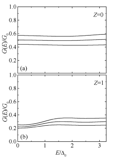
Figure 2: Differential conductance spectra of an FSF junction with (a) $Z=0$ and (b) $Z=1$, for a thin S layer ($d_{s}k_{\rm F}=10^{3}$), $X=0.5$, and three relative orientations of magnetizations: $\alpha=0$, $\alpha=\pi/2$, and $\alpha=\pi$ (top to bottom).

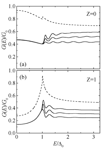
Figure 3: Differential conductance spectra of an FSF junction with (a) $Z=0$ and (b) $Z=1$, for a thick S layer ($d_{s}k_{\rm F}=10^{4}$), $X=0.5$, and three relative orientations of magnetizations: $\alpha=0$, $\alpha=\pi/2$, and $\alpha=\pi$ (top to bottom). The spectra of the corresponding FIS junctions (generalized BTK resultsBozovicB ) are shown for comparison (dashed lines).

When voltage $V$ is applied to the junction symmetrically, the charge current density can be written in the formYamashita67 ; Lambert ; Zheng

$$J(V) = \frac{e}{(2\pi)^{3}\hbar}\int\limits_{-\infty}^{\infty}{\rm d}E\sum_{\sigma=\uparrow,\downarrow}P_{\sigma}\times$$

$$\times\int{\rm d}^{2}{\bf k}_{||,\sigma}\left(1+A_{\sigma}-B_{\sigma}+C_{\sigma}-D_{\sigma}\right)\delta f({\bf k},V)$$

$$= \frac{e}{4\pi^{3}\hbar}\int\limits_{-\infty}^{\infty}{\rm d}E\sum_{\sigma=\uparrow,\downarrow}P_{\sigma}\times$$

$$\times\int{\rm d}^{2}{\bf k}_{||,\sigma}\left(A_{\sigma}+C_{\sigma}\right)\delta f({\bf k},V),$$ (21)

where $P_{\sigma}=(1+\rho_{\sigma}X)/2$ with $X=h_{0}/E_{\rm F}$, and $\delta f({\bf k},V)$ is the asymmetric part of the nonequilibrium distribution function of current carriers. In the last equality the normalization condition, Eq. (18), was taken into account. Without solving the suitable transport equation we take $\delta f({\bf k},V)=f_{0}(E-eV/2)-f_{0}(E+eV/2)$, where $f_{0}$ is the Fermi-Dirac distribution function.Tinkham ; BTK In this approach, the charge current per orbital transverse channel is given by

$$I(V)=\frac{1}{e}\int\limits_{-\infty}^{\infty}{\rm d}E\left[f_{0}(E-eV/2)-f_{0}(E+eV/2)\right]G(E),$$ (22)

where

$$G(E)=G_{0}\sum_{\sigma=\uparrow,\downarrow}P_{\sigma}\int\frac{{\rm d}^{2}{\bf k}_{||,\sigma}}{2\pi k_{\rm F}^{2}}\left(A_{\sigma}+C_{\sigma}\right)$$ (23)

is differential charge conductance at zero temperature and $G_{0}=e^{2}/\pi\hbar$ is the conductance quantum.

One can see that Eq. (23) is a simple generalization of the Landauer formula,Landauer with terms that take into account transmission of the current through Cooper pairs and quasiparticles. For $E<\Delta$, the subgap transmission of quasiparticles (without conversion into Cooper pairs) suppresses the Andreev reflection, while for $E>\Delta$ all the probabilities oscillate with $E$ and $d_{s}$ due to the interference of incoming and outgoing particles.

The influence of the exchange interaction and relative orientation of magnetizations on the conductance spectra is illustrated for $X=0.5$ and $Z=0$, for thin ($d_{s}k_{\rm F}=10^{3}$, Fig. 2) and thick ($d_{s}k_{\rm F}=10^{4}$, Fig. 3) S films. In all the illustrations the bulk value of superconducting pair potential is characterized by $\Delta_{0}/E_{\rm F}=10^{-3}$, which corresponds to $\xi_{0}k_{\rm F}=(2/\pi)\cdot 10^{3}$. For thin S layers, $d_{s}k_{\rm F}\lesssim 10^{3}$, the bulk value $\Delta_{0}$ is replaced by the averaged self-consistent pair potential, calculated in Ref. BozovicEPL, . The spin-polarized subgap transmission of quasiparticles, and consequently a strong suppression of the Andreev reflection, are significant in junctions with thin S films, whereas the conductance oscillations above the gap become pronounced as $d_{s}$ is increased. The magnetoresistance is apparent, as conductance is greater for the P ($\alpha=0$) than for the AP ($\alpha=\pi$) alignment. The presence of non-collinear magnetizations ($\alpha=\pi/2$) does not lead to any nonmonotonicity in the conductance spectra with respect to collinear cases ($\alpha=0$ and $\alpha=\pi$) – the values for $\alpha=\pi/2$ simply fall in between the P and AP curves. Moreover, it can be seen that the conductances for $E>\Delta$ oscillate in phase for $\alpha=0$, $\alpha=\pi/2$, and $\alpha=\pi$, Fig. 3(a). For thin S films ($d_{s}k_{\rm F}\lesssim 10^{3}$) transmission of the spin polarized current and suppression of Andreev reflection are still dominant at energies below $\Delta$, Fig. 2(a). The conductance spectra exhibit similar behavior for finite transparency of the interfaces. This is illustrated for weak non-transparency [$Z=1$, Figs. 2(b) and 3(b)]. From both Figs. 2 and 3 it can be seen that conductances attain their high-energy values, corresponding to conductances of an FNF double junction, when $E$ is of the order of several $\Delta$.

IV Magnetoresistance

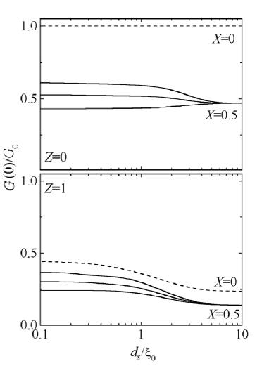
Figure 4: Zero-bias conductance of an FSF junction with $Z=0$ (top panel) and $Z=1$ (bottom panel) at zero temperature, as a function of the normalized S layer thickness $d_{s}/\xi_{0}$, for $X=0.5$, and three relative orientations of magnetizations: $\alpha=0$, $\alpha=\pi/2$, and $\alpha=\pi$ (top to bottom). The corresponding NSN values ($X=0$) are shown for comparison (dashed lines).

In clean FSF structures electrons propagating from F to S layer are not necessarily converted into Cooper pairs. Moreover, part of them has always a non-zero probability of being directly transmitted from one F electrode to the other, even at the voltage below $2\Delta/e$.BozovicB ; Yamashita67 This probability increases with decreasing $d_{s}$. As the applied voltage is increased, the conductance spectrum starts to resemble the one of an FNF junction. Fig. 4 shows the zero-bias voltage $G(0)$ as a function of normalized thickness of the S layer, $d_{s}/\xi_{0}$, for three relative orientations of magnetic moments: $\alpha=0$, $\alpha=\pi/2$, and $\alpha=\pi$. It can be seen that mutual differences between the corresponding values of $G(0)$ are larger the thinner the S layers are. At thicknesses of the order of the superconducting coherence length ($d_{s}/\xi_{0}\sim 1$) these differences slowly disappear, and vanish completely at $d_{s}/\xi_{0}\approx 5$. The increase of the normal reflection probability with $d_{s}$ is more rapid than the increase of the Andreev reflection probability if the insulating barriers were present in the junction. Consequently, zero-bias conductances are more sensitive to $d_{s}$ in the junctions without ($Z=1$) than in those with the full transparency ($Z=0$), as can be seen in Fig. 4.

For hybrids with thin S layers ($d_{s}k_{\rm F}\sim 10^{3}$ or less) zero-bias conductance decreases monotonously when $\alpha$ changes from $0$ to $\pi$ (Fig. 5), both for $Z=0$ and $Z=1$. If the S layers are thick ($d_{s}k_{\rm F}\sim 10^{4}$ or greater), $G(0)$ no longer depends on $\alpha$: the Andreev reflection dominates at energies close to the Fermi level, while the probability of direct transmission from any of the F layers through the superconductor is negligible, independently of mutual orientation of magnetizations. At energies above the gap, dependence of $G(E)$ on $\alpha$ is also monotonous, with values close to those for the corresponding FNF junction.

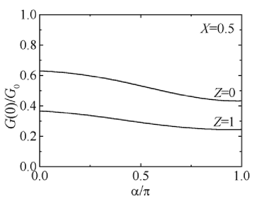
Figure 5: Zero-bias conductance of an FSF junction with $Z=0$ and $Z=1$ at zero temperature, as a function of the relative orientation of magnetizations $\alpha$, for $X=0.5$ and thin S layer, $d_{s}k_{\rm F}=10^{3}$.

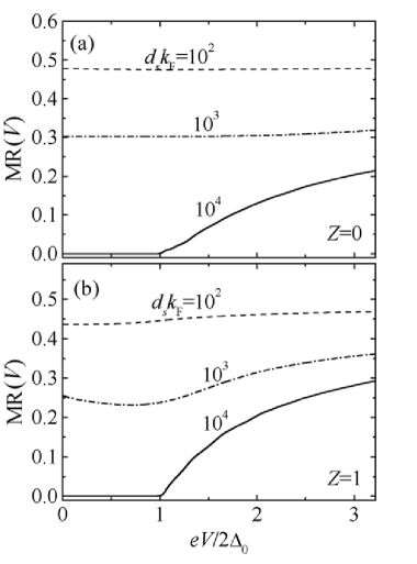
Figure 6: Magnetoresistance of an FSF junction with (a) $Z=0$ and (b) $Z=1$ at zero temperature, as a function of the applied voltage, for $X=0.5$, and ultrathin, thin, and thick S film, $d_{s}k_{\rm F}=10^{2},~{}10^{3},~{}10^{4}$, respectively.

Magnetoresistance is defined as

$${\rm MR}\equiv\frac{R_{\rm AP}-R_{\rm P}}{R_{\rm P}},$$ (24)

where $R_{\rm P(AP)}=V/I_{\rm P(AP)}$ is the junction resistance in P (AP) alignment of magnetizations. In Fig. 6, MR is shown as a function of bias applied symmetrically at the ends of an FSF junction with $Z=0$ and $Z=1$, for $X=0.5$ and three values of $d_{s}k_{\rm F}$: $10^{2}$, $10^{3}$, and $10^{4}$. The main characteristic of junctions with thin S layers ($d_{s}k_{\rm F}\sim 10^{2}-10^{3}$) is the dominance of direct transmission over Andreev reflection. Also, the average number of quasiparticles converted to Cooper pairs is small, independently of voltage, making the number of up spins that cross from one F layer to the other much greater than the corresponding down spins. This difference is greater in the P than in the AP alignment of magnetizations, leading to a magnetoresistance that gets more pronounced as the S layer becomes thinner. Conversely, in junctions with a thick S layer ($d_{s}k_{\rm F}\sim 10^{4}$), direct transmission probability is very low and hence most of the electrons that enter the S layer at energies below $\Delta$ are converted into Cooper pairs of net spin zero. Thus, for the electrons in one F layer the influence of the opposite F layer becomes practically negligible, and therefore ${\rm MR}\simeq 0$ for $eV/2\Delta_{0}\leq 1$. At higher voltages, $eV/2\Delta_{0}>1$, MR rises practically monotonously due to a gradual increase of direct transmission.

Therefore, magnetoresistance of clean FSF junctions exhibits a strong dependence on the S layer thickness, even at a low bias. The MR is always more pronounced if the exchange field is stronger. However, it decreases towards zero with increasing $d_{s}$ due to the dominance of supercurrent over the normal current.

V Spin-triplet correlations

A peculiar property of proximity of singlet-pairing superconductors and inhomogeneous ferromagnetic metals is inducement of triplet correlations between electron-hole pairs of equal spin orientations.BVE_rev These correlations also exist in systems with locally homogeneous exchange fields of non-collinear configuration.VBE Triplet correlations in F–S hybrids only resemble those of magnetic superconductors: while in the latter the Cooper pairs could be truly spin-triplet, in the former they remain singlet despite the presence of both singlet and triplet components of anomalous Green’s function.

To study the triplet correlations in clean FSF junctions we solve the Gor’kov equations generalized to take into account non-collinearity of magnetizations in the F layers. In this case, the net Green’s function $\check{\mathcal{G}}({\bf r_{1}},{\bf r_{2}})$ is a $(2\times 2)\otimes(2\times 2)$ matrix in the Nambu space. The Gor’kov equations can be compactly written as

$$\left(E\check{\mathbf{1}}-\check{\cal{H}}\right)\check{\mathcal{G}}({\bf r_{1}},{\bf r_{2}})=\delta({\bf r_{1}}-{\bf r_{2}})\check{\mathbf{1}},$$ (25)

where $\check{\cal{H}}$ is given by Eq. (3), while $\check{\mathbf{1}}$ is the unity matrix in the Nambu space. As the system of our interest is part-by-part homogeneous, in each layer of the junction the components of the matrix Green’s function $\check{\mathcal{G}}$ are functions of the relative coordinate ${\bf r}\equiv{\bf r_{1}}-{\bf r_{2}}$. It consists of four matrix blocks,

$$\check{\mathcal{G}}=\left(\begin{array}[]{cc}\widehat{G}^{+}&\widehat{F}\\ \widehat{F}^{\ast}&\widehat{G}^{-}\end{array}\right).$$ (26)

Here, we are interested only in the anomalous block

$$\widehat{F}=\left(\begin{array}[]{cc}F_{\uparrow\downarrow}&F_{\uparrow\uparrow}\\ F_{\downarrow\downarrow}&F_{\downarrow\uparrow}\end{array}\right).$$ (27)

The antisymmetric combination $(F_{\uparrow\downarrow}-F_{\downarrow\uparrow})/2$ describes singlet correlations, while the symmetric functions $(F_{\uparrow\downarrow}+F_{\downarrow\uparrow})/2$, $F_{\uparrow\uparrow}$, and $F_{\downarrow\downarrow}$ are related to triplet correlations. If the exchange field ${\bf h}({\bf r})$ has the same direction in the left and the right F layer ($\alpha=0$), then without loss of generality we can choose this to be direction of the $z$ axis, see Fig. 1. The blocks $\widehat{H}_{0}({\bf r})-{\bf h}({\bf r})\cdot\widehat{\bm{\sigma}}$ in $\check{\cal H}$ are then diagonal, and thus only the singlet correlations are present. The function $F=F_{\uparrow\downarrow}=F_{\downarrow\uparrow}$ is then the usual pair amplitude, while $F_{\uparrow\uparrow}=F_{\downarrow\downarrow}=0$. In general, however, it can be the case that $0<\alpha<\pi$. Then, the functions $F_{\uparrow\downarrow}$ and $F_{\downarrow\uparrow}$ are different, while $F_{\uparrow\uparrow}$ and $F_{\downarrow\downarrow}$ are non-zero, leading to existence of triplet correlations.

For ferromagnets, where $\Delta=0$, Eq. (25) reduces to

$$\left(E\widehat{\bf 1}-\widehat{H}_{+}({\bf r})\right)\widehat{F}({\bf r})=0.$$ (28)

General solution of this equation for the right F layer are

$$F_{\uparrow\downarrow} = \cos(\alpha/2)C_{1}e^{ik^{+}_{\uparrow}x}+\cos(\alpha/2)C_{2}e^{-ik^{+}_{\uparrow}x}$$

$$+i\sin(\alpha/2)C_{3}e^{ik^{+}_{\downarrow}x}+i\sin(\alpha/2)C_{4}e^{-ik^{+}_{\downarrow}x},$$ (29)

$$F_{\downarrow\downarrow} = i\sin(\alpha/2)C_{1}e^{ik^{+}_{\uparrow}x}+i\sin(\alpha/2)C_{2}e^{-ik^{+}_{\uparrow}x}$$

$$+\cos(\alpha/2)C_{3}e^{ik^{+}_{\downarrow}x}+\cos(\alpha/2)C_{4}e^{-ik^{+}_{\downarrow}x},$$ (30)

$$F_{\downarrow\uparrow} = i\sin(\alpha/2)C_{5}e^{ik^{-}_{\uparrow}x}+i\sin(\alpha/2)C_{6}e^{-ik^{-}_{\uparrow}x}$$

$$+\cos(\alpha/2)C_{7}e^{ik^{-}_{\downarrow}x}+\cos(\alpha/2)C_{8}e^{-ik^{-}_{\downarrow}x},$$ (31)

$$F_{\uparrow\uparrow} = \cos(\alpha/2)C_{5}e^{ik^{-}_{\uparrow}x}+\cos(\alpha/2)C_{6}e^{-ik^{-}_{\uparrow}x}$$

$$+i\sin(\alpha/2)C_{7}e^{ik^{-}_{\downarrow}x}+i\sin(\alpha/2)C_{8}e^{-ik^{-}_{\downarrow}x},$$ (32)

modulo phase factor $\exp(i{\bf k}_{||,\sigma}\cdot{\bf r})$. Solutions in the left F layer are obtained if we substitute $\alpha$ by $-\alpha$, and use a different set of constants, $C_{9},\ldots,C_{16}$. To find the complete set of unknown constants $C_{1},\ldots,C_{16}$ we have to use the continuity of $F_{\sigma\sigma^{\prime}}$ and its derivative at the S-F interfaces. However, to apply the boundary conditions at $x=\pm d_{s}/2$ we need to find solutions for $F_{\sigma\sigma^{\prime}}$ inside the superconductor, where $G_{\sigma\sigma^{\prime}}$ and $F_{\sigma\sigma^{\prime}}$ are coupled through the pair potential $\Delta({\bf r})$. To remain within a tractable analytical procedure, we use a simpler method which is sufficient for qualitative discussion. First, we eliminate eight out of sixteen constants using condition that holds at the outer boundaries,

$$F_{\sigma\sigma^{\prime}}\Big{|}_{x=\pm(d_{s}/2+d_{f})}=0.$$ (33)

Then, we connect these functions with corresponding solutions in the S layer, which for this purpose we treat as unknown parameters, defined as

$$F_{\uparrow\downarrow}\Big{|}_{x=\pm d_{s}/2}=A_{1},$$ (34)

$$F_{\downarrow\uparrow}\Big{|}_{x=\pm d_{s}/2}=A_{2},$$ (35)

$$F_{\uparrow\uparrow}\Big{|}_{x=\pm d_{s}/2}=B_{1},$$ (36)

$$F_{\downarrow\downarrow}\Big{|}_{x=\pm d_{s}/2}=B_{2}.$$ (37)

Note that the functions $F_{\sigma\sigma^{\prime}}$ depend on $E$, ${\bf k_{||}}$, and $x$. In order to describe the spatial variation of triplet components we introduce the pair amplitudes

$$f_{\sigma\sigma^{\prime}}(x)=N(0)\int_{0}^{\infty}{\rm d}E\int\frac{{\rm d}^{2}{\bf k}_{||,\sigma}}{2\pi k_{\rm F}^{2}}F_{\sigma\sigma^{\prime}}(E,{\bf k_{||,\sigma}},x),$$ (38)

where $N(0)$ is density of states at the Fermi level. Using these functions, we can further constructBVE_rev

$$f_{0}(x) = \frac{1}{2}\left[f_{\uparrow\downarrow}(x)+f_{\downarrow\uparrow}(x)\right],$$

$$f_{1}(x) = f_{\uparrow\uparrow}(x)~{}=~{}f_{\downarrow\downarrow}(x),$$ (39)

$$f_{3}(x) = \frac{1}{2}\left[f_{\uparrow\downarrow}(x)-f_{\downarrow\uparrow}(x)\right].$$

The following symmetries have to hold: $f_{0}(-x)=f_{0}(x)$, $f_{1}(-x)=-f_{1}(x)$, and $f_{3}(-x)=f_{3}(x)$. The function $f_{3}$ describes singlet, while $f_{0}$ and $f_{1}$ describe triplet correlations in the system. The function $f_{0}$ corresponds to electron-hole pairs of zero net spin orientation, while $f_{1}$ corresponds to pairs of net spin orientation equal to $\pm 1$. The $f_{3}$ component exists even when the exchange field is absent. Both $f_{3}$ and $f_{0}$ fall off rapidly in a ferromagnet: characteristic decay lengths are of the order of $\xi_{f}=\sqrt{\hbar D_{f}/h_{0}}$ in diffusive, and $\xi_{f}=\hbar v_{\rm F}/h_{0}$ in ballistic heterostructures, where $D_{f}$ is a diffusion constant of a dirty ferromagnet. In diffusive FSF junctions these components are of a short range, since the exchange field tends to align spins, while $f_{1}$ is of a long range and monotonically decaying.EfetovFSF Here, we will argue that in clean FSF hybrids $f_{1}$ can be of the same range as $f_{3}$, and no long-range monotonically decaying triplet correlations are generated.

If we assume that the F layers are bulk, $d_{f}\gg d_{s}$, and focus on correlations in the vicinity of the S-F interfaces, $|x|\gtrsim d_{s}/2$, then any plain wave of the form $e^{\pm ik^{\pm}_{\sigma}d_{f}}$ will be rapidly oscillating with respect to $e^{\pm ik^{\pm}_{\sigma}x}$. Therefore, the most important contribution to the integral of $F_{\sigma\sigma^{\prime}}$ over $E$ in Eq. (38) is from the energies close to $E=0$. The energy dependence in the wavevectors is thus negligible, and we can write $k^{\pm}_{\sigma}\simeq k^{\pm}_{\sigma}(E=0)\equiv k_{\sigma}$. Within this approximation the number of undetermined coefficients, defined by Eqs. (34)–(37), can be further reduced by applying the symmetries $f_{\uparrow\uparrow}(x)=f_{\downarrow\downarrow}(x)$ and $f_{\uparrow\downarrow}(x)=-f_{\downarrow\uparrow}(x)$ that now hold. Hence, $A_{1}=-A_{2}\equiv A$ and $B_{1}=B_{2}\equiv B$. Performing the integration over ${\bf k}_{||,\sigma}$ in Eq. (38), we finally obtain the following set of expressions for the pair amplitudes of the right F layer

$$f_{0}(x) = 0,$$ (40)

$$f_{1}(x) = B{\cal{I}}(\widetilde{x})+i\sin\alpha A{\cal{J}}(\widetilde{x}),$$ (41)

$$f_{3}(x) = A{\cal{I}}(\widetilde{x})-i\sin\alpha B{\cal{J}}(\widetilde{x}).$$ (42)

where $\widetilde{x}\equiv x-d_{s}/2$ is the relative distance from the right S-F interface. In Eqs. (40)–(42) we have introduced the auxiliary functions

$${\cal{I}}(\widetilde{x}) = \cos^{2}\left(\frac{\alpha}{2}\right){\cal{Q}}_{\uparrow}(\widetilde{x})+\sin^{2}\left(\frac{\alpha}{2}\right){\cal{Q}}_{\downarrow}(\widetilde{x}),$$ (43)

$${\cal{J}}(\widetilde{x}) = {\cal{Q}}_{\uparrow}(\widetilde{x})-{\cal{Q}}_{\downarrow}(\widetilde{x}),$$ (44)

where

$${\cal{Q}}_{\sigma}(\widetilde{x})=\int\frac{{\rm d}^{2}{\bf k}_{||,\sigma}}{2\pi k_{\rm F}^{2}}\frac{\sin\left[k_{\sigma}\left(d_{f}-\widetilde{x}\right)\right]}{\sin\left(k_{\sigma}d_{f}\right)}.$$ (45)

The function ${\cal{I}}(\widetilde{x})$ is even and has a maximum at the interfaces, ${\cal{I}}(0)=1$, while ${\cal{J}}(\widetilde{x})$ is odd, with ${\cal{J}}(0)=0$. The expressions for the pair amplitudes for the left F layer are straightforwardly obtained by substitutions $\alpha\rightarrow-\alpha$ and $\widetilde{x}\rightarrow-\widetilde{x}$. For $\alpha=\pi/2$ the auxiliary functions, Eqs. (43) and (44), then simplify to

$${\cal{I}}(\widetilde{x}) \simeq 2\left\{\frac{\sin(\kappa\widetilde{x})}{\kappa\widetilde{x}}-\frac{1}{2}\left[\frac{\sin(\kappa\widetilde{x}/2)}{(\kappa\widetilde{x}/2)}\right]^{2}\right\},$$ (46)

$${\cal{J}}(\widetilde{x}) \simeq \frac{\sin(\kappa\widetilde{x})}{(\kappa\widetilde{x})^{2}}-\frac{\cos(\kappa\widetilde{x})}{\kappa\widetilde{x}},$$ (47)

where $\kappa\equiv k_{{\rm F}\uparrow}-k_{{\rm F}\downarrow}$ is the difference between the Fermi wavenumbers for the two spin subbands,

$$\kappa=k_{\rm F}\left[(1+X)^{1/2}-(1-X)^{1/2}\right],$$ (48)

and, as before, $X=h_{0}/E_{\rm F}$. The approximated functions ${\cal{I}}(\widetilde{x})$ and ${\cal{J}}(\widetilde{x})$, given by Eqs. (46) and (47), are shown in Fig. 7 for $X=0.5$.

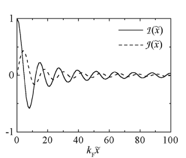
Figure 7: The functions ${\cal{I}}(\widetilde{x})$ (solid curve) and ${\cal{J}}(\widetilde{x})$ (dashed curve), under approximation $d_{f}\gg d_{s}$, shown for $\alpha=\pi/2$ and $X=0.5$.

Under the assumptions made, the unknown parameters $A$ and $B$ in Eqs. (41) and (42) will depend on $X$ and $\alpha$. If $X=0$ and/or $\alpha=0,\pi$ then $B=0$, since the triplet correlations are absent in these cases. From Eqs. (40)–(42) we can draw the following conclusions concerning triplet correlations in clean FSF heterostructures. The function $f_{0}$ is approximately zero inside the F layers. Since this function can only be generated by the exchange field it also cannot exist in the S layer. The singlet correlations, captured in $f_{3}$, consist of two terms. If $\alpha=0$ or $\pi$, $f_{3}$ reduces to $A{\cal{I}}(\widetilde{x})$. This term has a decay length $2\pi/\kappa\sim\xi_{f}$. Thus, the range of singlet correlations increases with decreasing strength of the exchange field. In special case of an NSN junction ($X=0$) we obtain a well-known result that singlet pair amplitude monotonically decays into the N layer.Valls04 For $X\neq 0$ and non-collinear magnetizations two components of the triplet pair amplitude $f_{1}$ oscillate on the same scale and with the same decay length.

We conclude that in clean FSF junctions at zero temperature both singlet and triplet pair correlations in ferromagnets are oscillating and power-law decaying with the distance from S-F interfaces. Physical intuition behind this result is that in such systems there exists only one characteristic length determining decay of correlations in the ferromagnets, which weakly depends on excitation energy $E$. This stands in a contrast with findings for diffusive FSF hybrids where two characteristic lengths are present: $\xi_{f}$ and $\xi_{\omega}=\sqrt{D_{f}/2\hbar|\omega|}$, where $\omega=(2n+1)\pi k_{\rm B}T$. At temperatures just below the critical one for the superconducting phase transition, $T<T_{c}$, the two lengths set up two different scales, $\xi_{\omega}\sim\sqrt{\hbar D_{f}/2\pi k_{B}T_{c}}\gg\xi_{f}$. Note that $\xi_{\omega}$ is also the length that determines the decay of singlet component in nonmagnetic normal metal.

VI Conclusion

We have studied the influence of misorientation of magnetizations on the properties of ballistic transport in clean FSF trilayers. By solving the Bogoliubov–de Gennes equation we have derived generalized expressions for probabilities of processes that charge carriers undergo. We use these probabilities to compute differential conductances for arbitrary orientation of magnetic moments and interface transparencies. Preferability of direct quasiparticle transmission to the Andreev reflection in thin S layers and more prominent resonant oscillations in thick S films are the main consequences of quantum interference in clean heterostructures. The subgap conductance is larger for P than for AP alignment as a result of strong magnetoresistive effect in thin S layers: when the S layer thickness is less or comparable to the superconducting coherence length the direct transmission of spin polarized quasiparticles across the superconductor becomes a dominant transport mechanism. However, we show that no extraordinary effects arise when the relative orientation of magnetizations is between parallel and antiparallel – the spectra for intermediary angles simply fall in between those for P and AP alignment.

From the obtained results we can further draw some general conclusions about the nature of ballistic transport in clean FSF trilayers with inhomogeneous magnetizations. Firstly, the zero-bias conductance depends on the relative orientation of magnetizations only in heterostructures with thin superconducting layers, decreasing monotonously when tuning from P to AP alignment. Secondly, magnetoresistance displays qualitatively different voltage dependance for thin and for thick superconducting layers due to different quasiparticle spectra which tends to gapless or bulk, respectively. Thirdly, magnetoresistance increases with the thickness of the S layer and vanishes eventually. The effect is more pronounced for strong exchange fields and transparent interfaces.

Non-collinearity of magnetizations leads to formation of spin-triplet pair correlations in FSF structures. Unlike the diffusive case, where the triplet correlations have a long-range and monotonically decaying component, we have shown that in clean ferromagnet-superconductor hybrids these correlations are oscillating and power-law decaying with the distance from S-F interfaces, similarly to the usual singlet correlations. This similarity in behavior of singlet and triplet pair correlations induced in ferromagnets is the main reason why the transport properties of clean FSF junctions have monotonic dependence on the angle between magnetizations. These findings suggest that any spectacular features of triplet correlations are highly unlikely to occur in clean FSF structures.

References

- (1) A. I. Buzdin, Rev. Mod. Phys. 77, 935 (2005).
- (2) I. F. Lyuksyutov and V. L. Pokrovsky, Adv. Phys. 54, 67 (2005).
- (3) F. S. Bergeret, A. F. Volkov, and K. B. Efetov, Rev. Mod. Phys. 77, 1321 (2005).
- (4) L. N. Bulaevskii, V. V. Kuzii, and A. A. Sobyanin, Pis’ma Zh. Éksp. Teor. Fiz. 25, 314 (1977) [JETP Lett. 25, 290 (1977)].
- (5) P. Fulde and A. Ferrel, Phys. Rev. 135, A550 (1964); A. Larkin and Y. Ovchinnikov, Sov. Phys. JETP 20, 762 (1965).
- (6) A. I. Buzdin, L. N. Bulaevskii, and S. V. Paniukov, Pis’ma Zh. Éksp. Teor. Fiz. 35, 147 (1982) [JETP Lett. 35, 178 (1982)].
- (7) Z. Radović, M. Ledvij, L. Dobrosavljević-Grujić, A. I. Buzdin, and J. R. Clem, Phys. Rev. B 44, 759 (1991).
- (8) A. I. Buzdin and M. V. Kupriyanov, Pis’ma Zh. Éksp. Teor. Fiz. 52, 1089 (1990) [JETP Lett. 52, 487 (1990)].
- (9) E. A. Demler, G. B. Arnold, and M. R. Beasley, Phys. Rev. B 55, 15 174 (1997).
- (10) L. R. Tagirov, Physica C 307, 145 (1998).
- (11) Ya. V. Fominov, N. M. Chtchelkatchev, and A. A. Golubov, Phys. Rev. B 66, 014507 (2002).
- (12) A. Bagrets, C. Lacroix, and A. Vedyayev, Phys. Rev. B 68, 054532 (2003).
- (13) T. Kontos, M. Aprili, J. Lesueur, and X. Grison, Phys. Rev. Lett. 86, 304 (2001).
- (14) V. V. Ryazanov, V. A. Oboznov, A. Yu. Rusanov, A. V. Veretennikov, A. A. Golubov, and J. Aarts, Phys. Rev. Lett. 86, 2427 (2001).
- (15) J. S. Jiang, D. Davidović, D. H. Reich, and C. L. Chien, Phys. Rev. Lett. 74, 314 (1995).
- (16) L. Lazar, K. Westerholt, H. Zabel, L. R. Tagirov, Yu. V. Goryunov, N. N. Garif yanov, and I. A. Garifullin, Phys. Rev. B 61, 3711 (2000).
- (17) I. A. Garifullin, D. A. Tikhonov, N. N. Garif yanov, L. Lazar, Yu. V. Goryunov, S. Ya. Khlebnikov, L. R. Tagirov, K. Westerholt, and H. Zabel, Phys. Rev. B 66, 020505(R) (2002).
- (18) Y. Obi, M. Ikebe, and H. Fujishiro, Phys. Rev. Lett. 94, 057008 (2005).
- (19) L. R. Tagirov, Phys. Rev. Lett. 83, 2058 (1999).
- (20) I. Baladie, A. Buzdin, N. Ryzhanova, and A. Vedyayev, Phys. Rev. B 63, 054518 (2001).
- (21) J. Y. Gu, C.-Y. You, J. S. Jiang, J. Pearson, Ya. B. Bazaliy, and S. D. Bader, Phys. Rev. Lett. 89, 267001 (2002).
- (22) K. Westerholt, D. Sprungmann, H. Zabel, R. Brucas, B. Hjörvarsson, D. A. Tikhonov, and I. A. Garifullin, Phys. Rev. Lett. 95, 097003 (2005).
- (23) F. S. Bergeret, K. B. Efetov, and A. I. Larkin, Phys. Rev. B 62, 11872 (2000).
- (24) F. S. Bergeret, A. F. Volkov, and K. B. Efetov, Phys. Rev. Lett. 86, 4096 (2001).
- (25) A. Kadigrobov, R. I. Shekhter, and M. Jonson, Europhys. Lett. 54, 394 (2001); Fiz. Nizk. Temp. 27, 1030 (2001) [Low Temp. Phys. 27, 760 (2001)].
- (26) M. L. Kulić and I. M. Kulić, Phys. Rev. B 63, 104503 (2001).
- (27) A. F. Volkov, F. S. Bergeret, and K. B. Efetov, Phys. Rev. Lett. 90, 117006 (2003).
- (28) F. S. Bergeret, A. F. Volkov, and K. B. Efetov, Phys. Rev. B 69, 174504 (2004).
- (29) Ya. V. Fominov, A. A. Golubov, and M. Yu. Kupriyanov, Pis’ma Zh. Éksp. Teor. Fiz. 77, 609 (2003). [JETP Lett. 77, 510 (2003)].
- (30) R. S. Keizer, S. T. B. Goennenwein, T. M. Klapwijk, G. Miao, G. Xiao, and A. Gupta, Nature 439, 825 (2006).
- (31) V. Peña, Z. Sefrioui, D. Arias, C. Leon, J. Santamaria, M. Varela, S. J. Pennycook, and J. L. Martinez, Phys. Rev. B 69, 224502 (2004).
- (32) M. Eschrig, J. Kopu, J. C. Cuevas, and G. Schön, Phys. Rev. Lett. 90, 137003 (2003).
- (33) M. Božović and Z. Radović, Phys. Rev. B 66, 134524 (2002).
- (34) T. Yamashita, H. Imamura, S. Takahashi, and S. Maekawa, Phys. Rev. B 67, 094515 (2003).
- (35) M. Eschrig, J. Kopu, A. Konstandin, J. C. Cuevas, M. Fogelström, and G. Schön, Advances in Solid State Physics, vol. 44, pp. 533–546 (Springer-Verlag, Heidelberg, 2004).
- (36) T. Lofwander, T. Champel, J. Durst, and M. Eschrig, Phys. Rev. Lett. 95, 187003 (2005).
- (37) Z. C. Dong, Phys. Rev. B 72, 054517 (2005).
- (38) M. Fauré and A. I. Buzdin, Phys. Rev. Lett. 94, 187202 (2005).
- (39) M. Božović and Z. Radović, Europhys. Lett. 70, 513 (2005).
- (40) K. Halterman and O. T. Valls, Phys. Rev. B 72, 060514(R) (2005).
- (41) G. Bergmann, Phys. Rev. B 72, 134505 (2005).
- (42) A. Furusaki and M. Tsukada, Solid State Commun. 78, 299 (1991).
- (43) S. Russo, M. Kroug, T. M. Klapwijk, and A. F. Morpurgo, Phys. Rev. Lett. 95, 027002 (2005).
- (44) D. Beckmann, H. B. Weber, and H. v. Löhneysen, Phys. Rev. Lett. 93, 197003 (2004).
- (45) M. Božović and Z. Radović, in Proceedings of SPIE, vol. 4811, Superconducting and Related Oxides: Physics and nanoengineering V, edited by I. Božović and D. Pavuna (SPIE, Bellingham, WA, 2002), pp. 216-227; cond-mat/0207375.
- (46) C. Cohen-Tannoudji, B. Diu, and F. Laloe, Quantum Mechanics, (Hermann, Paris, 1977).
- (47) M. Tinkham, Introduction to Superconductivity, (McGraw-Hill, New York, 1996).
- (48) C. J. Lambert, J. Phys.: Condens. Matter 3, 6579 (1991).
- (49) Z. C. Dong, R. Shen, Z. M. Zheng, D. Y. Xing, Z. D. Wang, Phys. Rev. B 67, 134515 (2003).
- (50) G. E. Blonder, M. Tinkham, and T. M. Klapwijk, Phys. Rev. B 25, 4515 (1982).
- (51) R. Landauer, IBM J. Res. Dev. 1, 233 (1957).
- (52) F. S. Bergeret, A. F. Volkov, and K. B. Efetov, Phys. Rev. B 68, 064513 (2003).
- (53) K. Halterman and O. T. Valls, Phys. Rev. B 66, 224516 (2002); 69, 014517 (2004).