The Fermi-Hubbard model at unitarity

Abstract

We simulate the dilute attractive Fermi-Hubbard model in the unitarity regime using a diagrammatic determinant Monte Carlo algorithm with worm-type updates. We obtain the dependence of the critical temperature on the filling factor $\nu$ and, by extrapolating to $\nu\to 0$, determine the universal critical temperature of the continuum unitary Fermi gas in units of Fermi energy: $T_{c}/\varepsilon_{F}=0.152(7)$. We also determine the thermodynamic functions and show how the Monte Carlo results can be used for accurate thermometry of a trapped unitary gas.

1 Introduction

In recent years, ultracold atomic systems have served as a controlled and tunable toolbox for studying many-body quantum phenomena. The continuous tunability of the interaction by Feshbach resonances makes these systems ideal candidates to study the crossover from momentum space pairing in the Bardeen–Cooper–Schrieffer (BCS) theory to Bose-Einstein condensate (BEC) of fermions bound into molecules. This BCS-BEC crossover has been one of the most studied problems in recent experiments in both magnetic or optical traps [1, 2, 3, 4, 5, 6] and optical lattices [7].

Tuning across the Feshbach resonance, one traverses the whole range of the gas parameter $k_{F}a_{s}$, where $k_{F}$ is the Fermi momentum and $a_{s}$ is the s-wave scattering length. The regime of $k_{F}|a_{s}|\ll 1$ (negative $a_{s}$) is described by Bardeen–Cooper–Schrieffer (BCS) theory. At $k_{F}a_{s}\ll 1$ (positive $a_{s}$) fermions pair into bosonic molecules and form a Bose-Einstein condensate (BEC). At the microscopic scale, the BCS and BEC regimes are radically different; however, the macroscopic, and, in particular, critical behaviour is supposed to be qualitatively the same for the whole range of $k_{F}a_{s}$: the system undergoes the superfluid (SF) phase transition at a certain critical temperature. Separating the BCS and BEC extremes is the so-called unitarity point $(k_{F}a_{s})^{-1}\to 0$. It is worth noting that the unitarity regime is approximately realized in the inner crust of the neutron stars, where the neutron-neutron scattering length is nearly an order of magnitude larger than the mean interparticle separation [8].

The Fermi gas at unitarity is a peculiar case of a strongly interacting system with no interaction-related energy scale: the divergent scattering length and any related energy scale drop out completely. This gives rise to universality of the dilute gas properties, in the sense that the only relevant energy scale left in the system is given by the density, $n$. Because of this universality one obtains a unified description of such diverse systems as cold atoms in magnetic or optical traps, Fermi-Hubbard model in optical lattices and inner crusts of neutron stars.

The theoretical description of the Fermi gas in the BCS-BEC crossover regime is a major challenge, since the system features no small parameter on which one could build a theory in a rigorous way. The original analytical treatments were confined to zero temperature and were based on the extension of the BCS-type many-body wave function [9]. Most of the subsequent elaborations are also of mean-field type (with or without remedies for the effects of fluctuations) [10, 11, 12, 13, 14, 15, 16]. The accuracy and reliability of such approximations is questionable since they inevitably involve an uncontrollable approximation.

Numerical investigations of the unitary Fermi gases are hampered by the sign problem, inherent to any Monte Carlo (MC) simulations of fermion systems [17, 18]. One way of avoiding the sign problem at the expense of a systematic error is the fixed-node Monte Carlo framework, which has been used to study the ground state [19]. The systematic error of the fixed-node Monte Carlo depends on the quality of the variational ansatz for the nodal structure of the many-body wave function and is not known precisely. Only in a few exceptional cases can the sign problem be avoided without incurring systematic errors. One of such cases is given by fermions with attractive contact interaction, for which a number of sign-problem-free schemes has been introduced [20, 21, 22, 23]. Fortunately, this system can be tuned to the unitarity regime. Still, despite a number of calculations at finite temperature [24, 25, 26], an accurate description of the finite-temperature properties of the unitary Fermi gas is missing.

In the present paper, we simulate the Fermi-Hubbard model in the unitary regime by means of a determinant diagrammatic Monte Carlo method. By studying the dilute limit of the model, we extract properties of the homogeneous continuum Fermi gas. A brief summary of the main results has been given in Ref. [27]. Here we provide a detailed description of the Monte Carlo scheme and methods of data analysis. We also report new results relevant to experimental realizations of the Fermi-Hubbard model in optical lattices and trapped Fermi gases.

The Fermi-Hubbard model is defined by the Hamiltonian

$$H=H_{0}+H_{1},\\$$ (1.1a)

$$H_{0}=\sum_{\mathbf{k}\sigma}\left(\epsilon_{\mathbf{k}}-\mu\right)c^{\dagger}_{\mathbf{k}\sigma}c_{\mathbf{k}\sigma},\\$$ (1.1b)

$$H_{1}=U\sum_{\mathbf{x}}n_{\mathbf{x}\uparrow}n_{\mathbf{x}\downarrow}\;.$$ (1.1c)

Here $c^{\dagger}_{\mathbf{k}\sigma}$ is a fermion creation operator, $n_{\mathbf{x}\sigma}=c^{\dagger}_{\mathbf{x}\sigma}c_{\mathbf{x}\sigma}$, $\sigma=\uparrow,\downarrow$ is the spin index, $\mathbf{x}$ enumerates $L^{3}$ sites of the three-dimensional (3D) simple cubic lattice with periodic boundary conditions, the quasimomentum $\mathbf{k}$ spans the corresponding Brillouin zone, $\epsilon_{\mathbf{k}}=2t\sum_{\alpha=1}^{3}(1-\cos k_{\alpha}a)$ is the single-particle tight-binding spectrum, $a$ and $t$ are the lattice spacing and the hopping amplitude, respectively, $\mu$ stands for the chemical potential and $U<0$ is the on-site attraction. Without loss of generality we henceforth set $a$ and $t$ equal to unity; the effective mass at the bottom of the band is then $m=1/2$.

In Sec. 2 we will study the two-body problem at zero temperature, show how the Hubbard model can be used to study the continuum unitary gas and investigate the functional structure of lattice corrections to the continuum behaviour. In Sec. 3 we discuss the finite-temperature diagrammatic expansion for the Hubbard model (Sec. 3.1), and give a qualitative description of the Monte Carlo procedure to sum the diagrammatic series (Sec.3.2), with details of the updating procedures given in Appendix A. In order to extract the thermodynamic limit properties from MC data, we use finite-size scaling analysis described in Sec. 4. Section 5 gives an overview of the scaling functions describing thermodynamics of the unitary gas, and results are presented and discussed in Sec. 6.

2 Two-body problem

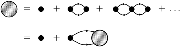
Figure 1: Diagrammatic series for the vertex insertion $\Gamma(\xi,\mathbf{p})$ (heavy dot). Small dots represent the bare Hubbard interaction $U$, and lines are the single-particle propagators.

Consider a quantum mechanical problem of two fermions at zero temperature described by the Hamiltonian (1.1a)–(1.1c) with $\mu=0$. The most straightforward way to tackle this problem is within the diagrammatic technique in the momentum-frequency representation [28, 29], which, in the present case, is built on four-point vertices, $U$, with two incoming (spin-$\uparrow$ and spin-$\downarrow$) and two outgoing (spin-$\uparrow$ and spin-$\downarrow$) ends, connected by single-particle propagators. The scattering of two particles is then described by a series of ladder diagrams [29, §16] shown in figure 1. Ladder diagrams can be summed by introducing the vertex insertion $\Gamma(\xi,\mathbf{p})$, which depends on frequency $\xi$ and momentum $\mathbf{p}$. Since $\Gamma(0,0)$ is proportional to the scattering amplitude, the unitarity limit corresponds to $\Gamma(\xi\to 0,\mathbf{p}\to\mathbf{0})\to\infty$. The summation depicted in figure 1 leads to

$$\Gamma^{-1}(\xi,\mathbf{p})=U^{-1}+\Pi(\xi,\mathbf{p})\;,$$ (1.1a)

where $\Pi(\xi,\mathbf{p})$ is the polarization operator (the integration is over the Brillouin zone):

$$\Pi(\xi,\mathbf{p})=\int_{\mathrm{BZ}}\frac{\rmd\mathbf{k}}{(2\pi)^{3}}\frac{1}{\xi+\epsilon_{\mathbf{p}/2+\mathbf{k}}+\epsilon_{\mathbf{p}/2-\mathbf{k}}}\;.$$ (1.1b)

It immediately follows from Eq. (1.1a) and (1.1b) that the unitary limit corresponds to $U=U_{*}$, where

$$U^{-1}_{*}=-\Pi(0,\mathbf{0})=-\int_{\mathrm{BZ}}\frac{\rmd\mathbf{k}}{(2\pi)^{3}}\,\frac{1}{2\epsilon_{\mathbf{k}}}\;.$$ (1.1c)

A straightforward numeric integration yields $U_{*}\approx-7.915t$.

In the limit of vanishing filling factor $\nu\to 0$ for the many-body problem of (1.1a)–(1.1c) the typical values of $\xi$ and $p$ are related to the Fermi energy $\xi\sim\epsilon_{F}\sim\nu^{2/3}$ and Fermi momentum $p\sim k_{F}\sim\nu^{2/3}$ and are small compared to the bandwidth and reciprocal lattice vector, respectively. In zero-th order with respect to $\nu$, the lattice system is identical to the continuum one. Indeed, by combining (1.1a), (1.1b) and (1.1c), we get

$$\Gamma^{-1}(\xi,\mathbf{p})=\int_{\mathrm{BZ}}\frac{\rmd\mathbf{k}}{(2\pi)^{3}}\left[\frac{1}{\xi+\epsilon_{\mathbf{p}/2+\mathbf{k}}+\epsilon_{\mathbf{p}/2-\mathbf{k}}}-\frac{1}{2\epsilon_{\mathbf{k}}}\right]\;,$$ (1.1d)

and observe that for small $\xi$ and $p$ one can replace $\varepsilon({\bf k})$ with $k^{2}$ and extend integration over $\rmd\mathbf{k}$ to the whole momentum space with the result

$$\Gamma^{-1}_{\mathrm{cont}}(\xi,\mathbf{p})=-\frac{m^{3/2}}{4\pi}\sqrt{\xi+\frac{p^{2}}{4m}}\;.$$ (1.1e)

With this form of $\Gamma_{\mathrm{cont}}$, and particle propagators based on the parabolic dispersion relation one recovers the continuum limit behaviour.

Now we are in a position to treat the lattice corrections. The first correction should come from $\Gamma$, not from propagators, since only in $\Gamma$ large momenta play a special role due to resonance in the two-particle channel. In the lowest non-vanishing order in $\xi$ and $\mathbf{p}$ we have (the summation over repeating subscripts is implied)

$$\Gamma^{-1}\approx-\int_{\mathrm{BZ}}{\rmd{\bf k}\over(2\pi)^{3}}\,\frac{\xi+(1/4)(\partial^{2}\varepsilon_{\mathbf{k}}/\partial k_{i}\partial k_{j})p_{i}p_{j}}{4\varepsilon_{\mathbf{k}}^{2}}\;.$$ (1.1f)

with the difference between the lattice and continuous model given by

$$\Gamma^{-1}-\Gamma^{-1}_{\mathrm{cont}}\;\approx\;\frac{\xi}{4}A+\frac{p^{2}}{16}B\;,$$ (1.1g)

where

$$A=\int{\rmd{\bf k}\over(2\pi)^{3}}\,{1\over(k^{2}/2m)^{2}}-\int_{\mathrm{BZ}}{\rmd{\bf k}\over(2\pi)^{3}}\,{1\over\varepsilon_{\mathbf{k}}^{2}}\;,$$ (1.1h)

$$B=\int{\rmd{\bf k}\over(2\pi)^{3}}\,{1/m\over(k^{2}/2m)^{2}}-\int_{\mathrm{BZ}}{\rmd{\bf k}\over(2\pi)^{3}}\,{(\partial^{2}\varepsilon_{\mathbf{k}}/\partial k_{x}\partial k_{x})\over\varepsilon_{\mathbf{k}}^{2}}\;.$$ (1.1i)

In the limit of $\xi\to 0$ and $p\to 0$, we have $\Gamma^{-1}\approx\Gamma^{-1}_{\mathrm{cont}}\sim k_{F}\sim\nu^{1/3}$, and $\Gamma^{-1}-\Gamma^{-1}_{\mathrm{cont}}\sim k_{F}^{2}\sim\nu^{2/3}$. Hence, the leading lattice correction is of the form

$$\frac{\Gamma(\xi,\mathbf{p})-\Gamma_{\mathrm{cont}}(\xi,\mathbf{p})}{\Gamma(\xi,\mathbf{p})}\;\sim\;\nu^{1/3}\;.$$ (1.1j)

Incidentally, Eqs. (1.1h) and (1.1i) hint into an intriguing possibility of completely suppressing the leading-order lattice correction by tuning the single-particle spectrum $\epsilon_{\mathbf{k}}$ so that $A=B=0$. We did not explore this possibility in the present study.

3 Determinant Diagrammatic Monte Carlo

The diagrammatic technique employed in the previous section is not particularly convenient for numerical studies. In this section, we briefly review the Matsubara technique and then present a Monte Carlo scheme of summing the resultant diagrammatic series.

3.1 Rubtsov’s representation

To construct a diagrammatic expansion for the model (1.1a)–(1.1c) we follow Refs. [22, 30] and consider the statistical operator in the coordinate—imaginary time representation. In the interaction picture we get:

$$\exp(-\beta H)\;=\;\exp(-\beta H_{0})\,\mathcal{T}_{\tau}\exp\left(-\int_{0}^{\beta}\,\rmd\tau H_{1}(\tau)\right)\;,$$ (1.1a)

where $\beta$ is an inverse temperature, $H_{1}(\tau)=e^{\tau H_{0}}H_{1}e^{-\tau H_{0}}$, and $\mathcal{T}_{\tau}$ stands for the imaginary time ordering.

Expanding Eq. (1.1a) in powers of $H_{1}$, one obtains for the partition function:

$$Z\;=\;\sum_{n=0}^{\infty}(-U)^{n}\sum_{\mathbf{x}_{1}\dots\mathbf{x}_{n}}\int_{0<\tau_{1}<\tau_{2}<\dots<\beta}\prod_{j=1}^{n}\rmd\tau_{j}\Tr\left[e^{-\beta H_{0}}\prod_{j=1}^{n}c_{\uparrow}^{\dagger}(\mathbf{x}_{j}\tau_{j})c_{\uparrow}(\mathbf{x}_{j}\tau_{j})c_{\downarrow}^{\dagger}(\mathbf{x}_{j}\tau_{j})c_{\downarrow}(\mathbf{x}_{j}\tau_{j})\right]\;.$$ (1.1b)

Expansion (1.1b) generates the standard set of Feynman diagrams. Graphically, the diagrams are similar to those of Sec. 2, and consist of the four-point vertices, $U$, connected by the single-particle propagators $G_{\sigma}^{(0)}(\mathbf{x}_{i}-\mathbf{x}_{j},\tau_{i}-\tau_{j};\mu,\beta)=-\Tr\left[\mathcal{T}_{\tau}e^{-\beta H_{0}}c_{\sigma}^{\dagger}(\mathbf{x}_{i}\tau_{i})c_{\sigma}(\mathbf{x}_{j}\tau_{j})\right]$. The $p$-th order of the perturbation theory is then graphically given by a set of $(p!)^{2}$ possible interconnections of vertices by propagators, see figure 2.

Figure 2: Diagrammatic series for the partition function. Upper line is the graphical representation of the series (1.1b), lower line depicts Eq. (1.1d). Diagram signs are shown explicitly.

The diagrammatic expansion (1.1b) is unsuitable for the direct Monte Carlo simulation since it has a sign problem built in: different terms in the series have different signs — a closed fermion loop brings in an extra minus sign [28]. The trick is to consider all diagrams of a given order $p$ with the fixed vertex configuration

$$\mathcal{S}_{p}=\{(\mathbf{x}_{j},\tau_{j}),~{}~{}j=1,\dots,p\}$$ (1.1c)

as one. This implies summation over the $(p!)^{2}$ ways of connecting vertices by propagators. Upon summation, Eq. (1.1b) takes on the form [22]:

$$Z=\sum_{p=0}^{\infty}(-U)^{p}\sum_{\mathcal{S}_{p}}\det\mathbf{A}^{\uparrow}(\mathcal{S}_{p})\det\mathbf{A}^{\downarrow}(\mathcal{S}_{p})\;,$$ (1.1d)

where

$$\sum_{\mathcal{S}_{p}}\equiv\sum_{\mathbf{x}_{1}\dots\mathbf{x}_{p}}\int_{0<\tau_{1}<\tau_{2}<\dots<\tau_{p}<\beta}\prod_{j=1}^{p}\rmd\tau_{j}\;,$$ (1.1e)

and $\mathbf{A}^{\sigma}(\mathcal{S}_{p})$ are the $p\times p$ matrices built on the single-particle propagators:

$$A^{\sigma}_{ij}(\mathcal{S}_{p})=G^{(0)}_{\sigma}(\mathbf{x}_{i}-\mathbf{x}_{j},\tau_{i}-\tau_{j})\;,~{}~{}~{}i,j=1,\dots,p\;.$$ (1.1f)

For equal number of spin-up and spin-down particles $\det\mathbf{A}^{\uparrow}\det\mathbf{A}^{\downarrow}=|\det\mathbf{A}|^{2}$, and the sign problem is absent. Graphically, Feynman diagrams in this representation are just collections of vertices, see figure 2. For future use, we define the set of all possible vertex configurations (1.1c) by $\mathfrak{S}^{(Z)}$, i.e., $\mathfrak{S}^{(Z)}=\{p,\{\mathcal{S}_{p}\}\}$.

The following two-point pair correlation function will prove useful:

$$G_{2}(\mathbf{x}\tau;\mathbf{x}^{\prime}\tau^{\prime})\;=\;\left\langle\,\mathcal{T}_{\tau}P(\mathbf{x},\tau)P^{\dagger}(\mathbf{x}^{\prime},\tau^{\prime})\,\right\rangle\;\equiv\;{g_{2}(\mathbf{x}\tau;\mathbf{x}^{\prime}\tau^{\prime})\over Z}\;,$$ (1.1g)

$$g_{2}(\mathbf{x}\tau;\mathbf{x}^{\prime}\tau^{\prime})\;=\;{\rm Tr}\,\mathcal{T}_{\tau}P(\mathbf{x},\tau)P^{\dagger}(\mathbf{x}^{\prime},\tau^{\prime})\,{\rm e}^{-\beta H}\;,$$ (1.1h)

where $P(\mathbf{x},\tau)$ and $P^{\dagger}(\mathbf{x}^{\prime},\tau^{\prime})$ are the pair annihilation and creation operators in the Heisenberg picture, respectively: $P(\mathbf{x},\tau)=c_{\mathbf{x}\uparrow}(\tau)c_{\mathbf{x}\downarrow}(\tau)$. The non-zero asymptotic value of $G_{2}(\mathbf{x}\tau;\mathbf{x}^{\prime}\tau^{\prime})$ as $|\mathbf{x}-\mathbf{x}^{\prime}|\to\infty$ is proportional to the condensate density.

Feynman diagrams for $g_{2}(\mathbf{x}\tau;\mathbf{x}^{\prime}\tau^{\prime})$ are similar to those for $Z$, but contain two extra elements: a pair of two-point vertices with two incoming (outgoing) ends which represent $P(\mathbf{x},\tau)$ ( $P^{\dagger}(\mathbf{x}^{\prime},\tau^{\prime})$ ), see figure 3. The vertex configurations for the correlation function (1.1g) slightly differ from those for the partition function (1.1c) by the presence of the two extra elements: the configuration space for Eq. (1.1g) is $\mathfrak{S}^{(G)}=\{p,\{\tilde{\mathcal{S}}_{p}\}\}$, with

$$\tilde{\mathcal{S}}_{p}=\{P(\mathbf{x},\tau),\,P^{\dagger}(\mathbf{x}^{\prime},\tau^{\prime}),\,(\mathbf{x}_{j},\tau_{j}),~{}~{}j=1,\dots,p\}\;.$$ (1.1i)

The partially summed diagrammatic expansion for $g_{2}(\mathbf{x}\tau;\mathbf{x}^{\prime}\tau^{\prime})$ is similar to Eq. (1.1d):

$$g_{2}(\mathbf{x}\tau;\mathbf{x}^{\prime}\tau^{\prime})=\sum_{p=0}^{\infty}(-U)^{p}\sum_{\tilde{\mathcal{S}}_{p}}\det\widetilde{\mathbf{A}}^{\uparrow}(\tilde{\mathcal{S}}_{p})\det\widetilde{\mathbf{A}}^{\downarrow}(\tilde{\mathcal{S}}_{p})\;,$$ (1.1j)

where $\widetilde{\mathbf{A}}^{\sigma}(\tilde{\mathcal{S}}_{p})$ is a $(p+1)\times(p+1)$ matrix which differs from Eq. (1.1f) only by that it has an extra row $i_{0}$ and an extra column $j_{0}$ such that $\widetilde{A}^{\sigma}_{ij_{0}}=G^{(0)}_{\sigma}(\mathbf{x}_{i}-\mathbf{x},\tau_{i}-\tau)$ and $\widetilde{A}^{\sigma}_{i_{0}j}=G^{(0)}_{\sigma}(\mathbf{x}^{\prime}-\mathbf{x}_{j},\tau^{\prime}-\tau_{j})$.

Figure 3: Diagrammatic series for the correlation function (1.1g). Diamonds represent the two-point creation/annihilation operators $P$ and $P^{\dagger}$.

Below we deal only with equal number of spin-up and spin-down fermions and (for the sake of brevity) suppress the spin indices wherever possible. We also peruse the generic notation (with superscripts) $\mathcal{D}(\mathcal{S}_{p})$ for $p$-th order terms of the diagrammatic expansions similar to (1.1d), e.g., $\mathcal{D}^{(Z)}(\mathcal{S}_{p})=(-U)^{p}\bigl{|}\det\mathbf{A}(\mathcal{S}_{p})\bigr{|}^{2}$. To simplify the notation we also omit superscripts if this does not lead to ambiguity.

3.2 Diagrammatic Monte Carlo and Worm algorithm

Equations (1.1d) and (1.1j) have similar general structure of a series of integrals and sums with ever increasing number of integration variables and summations. In Refs. [31, 32] it has been shown how to arrange a numerical procedure that sums such convergent series. To this end one considers the space of all possible vertex configurations $\mathfrak{S}$ ( for the series (1.1d) $\mathfrak{S}\equiv\mathfrak{S}^{(Z)}$, while for the series (1.1j) $\mathfrak{S}\equiv\mathfrak{S}^{(G)}$ ), with the “weight” $\mathcal{D}(\mathcal{S}_{p})$ associated with each element of the space. One then uses the Metropolis principle [33] to arrange a stochastic Markov process which sequentially generates vertex configurations $\mathcal{S}_{p}$ according to their weights $\mathcal{D}(\mathcal{S}_{p})$, thus sampling the space $\mathfrak{S}$. In the course of sampling, one also collects statistics for observables in the form of MC estimators, see Sec. 3.3.

The stochastic process consists of elementary MC updates performed on vertex configurations $\mathcal{S}_{p}$. The set of updates is problem-specific being restricted only by the requirements of (i) the ergodicity, i.e., given a particular diagram $\mathcal{S}_{p}$ it takes a finite number of steps to convert it into any other diagram $\mathcal{S}^{\prime}_{q}$, and (ii) detailed balance, i.e., relative contributions of diagrams $\mathcal{S}_{p}$ and $\mathcal{S}^{\prime}_{q}$ to the statistics is given by the ratio of their weights, $\mathcal{D}(\mathcal{S}_{p})/\mathcal{D}(\mathcal{S}^{\prime}_{q})$. The set of updates satisfying these requirements is not unique, the freedom is used to maximize the efficiency of simulations, as explained in detail in A.

In view of close similarity between the diagrammatic expansions (1.1d) and (1.1j) it is advantageous to construct a Monte Carlo process which samples these two series in a single simulation. This way one has access to both diagonal, e.g., energy, and off-diagonal properties, e.g., the superfluid response. An efficient way of performing such concurrent simulation is provided by the worm algorithm, which was originally devised for the worldline Monte Carlo simulations [34]. In the context of the diagrammatic determinant Monte Carlo, the generic worm algorithm principles imply the following. First, one works in the joint configuration space $\mathfrak{S}^{(Z)}\cup\mathfrak{S}^{(G)}$, accommodating diagrams (1.1c) and (1.1i). Second, all the updates are performed exclusively in terms of the two-point vertices $P(\mathbf{x},\tau)$ and $P^{\dagger}(\mathbf{x},\tau)$—through their creation/annihilation, motion, and “interactions” with adjacent vertices. The worm-type updating procedures are further detailed in A. Within the worm-algorithm framework, the configuration spaces $\mathfrak{S}^{(Z)}$ and $\mathfrak{S}^{(G)}$ are disjoint subsets of one extended configuration space. In what follows we will refer to them as $Z$-(or “diagonal”) and $G$-(or “off-diagonal”) sectors of the configuration space.

Formally, the extended configuration space corresponds to the generalized partition function

$$Z_{\mathrm{W}}\;=\;Z+\zeta\sum_{\mathbf{x},\mathbf{x}^{\prime}}\int_{0}^{\beta}\rmd\tau\int_{0}^{\beta}\rmd\tau^{\prime}g_{2}(\mathbf{x}\tau;\mathbf{x}^{\prime}\tau^{\prime})\;,$$ (1.1k)

where the value of $\zeta$ is arbitrary — it controls the relative statistics of $Z$- and $G$-sectors and the efficiency of simulation.

3.3 Monte Carlo estimators

Suppose we have an observable $X(\alpha)$, which depends on a set of variables $\alpha$, e.g. temperature and chemical potential. A MC estimator for the observable $X$ is an expression which, upon averaging over the sequence of MC configurations converges to the expectation value of $X(\alpha)$.

In accordance with Eq. (1.1k), the simplest worm-algorithm MC estimators are

$$\delta^{(Z)}(\mathcal{S}_{p})\;=\;\cases{1,&$\mathcal{S}_{p}\in\mathfrak{S}^{(Z)}$\; ,\\ 0,&$\widetilde{\mathcal{S}}_{p}\in\mathfrak{S}^{(G)}$\; ,\\ }$$ (1.1l)

and

$$\delta^{(G)}(\mathcal{S}_{p})\;=\;\cases{0,&$\mathcal{S}_{p}\in\mathfrak{S}^{(Z)}$\; ,\\ 1,&$\widetilde{\mathcal{S}}_{p}\in\mathfrak{S}^{(G)}$\; .\\ }$$ (1.1m)

Their MC averages are

$$\bigl{\langle}\delta^{(Z)}\bigr{\rangle}_{\mathrm{MC}}\;\longrightarrow\;Z/Z_{W}\;,$$ (1.1n)

and

$$\bigl{\langle}\delta^{(G)}\bigr{\rangle}_{\mathrm{MC}}\;\longrightarrow\;Z_{W}^{-1}\zeta\sum_{\mathbf{x},\mathbf{x}^{\prime}}\int_{0}^{\beta}\rmd\tau\int_{0}^{\beta}\rmd\tau^{\prime}\,g_{2}(\mathbf{x}\tau;\mathbf{x}^{\prime}\tau^{\prime})\;,$$ (1.1o)

where $\langle\dots\rangle_{\mathrm{MC}}$ denotes averaging over the set of stochastically generated configurations. In particular, for our purposes it will be quite useful that

$$\frac{\bigl{\langle}\delta^{(G)}\bigr{\rangle}_{\mathrm{MC}}}{\bigl{\langle}\delta^{(Z)}\bigr{\rangle}_{\mathrm{MC}}}\;\longrightarrow\;\zeta\sum_{\mathbf{x},\mathbf{x}^{\prime}}\int_{0}^{\beta}\rmd\tau\int_{0}^{\beta}\rmd\tau^{\prime}\,G_{2}(\mathbf{x}\tau;\mathbf{x}^{\prime}\tau^{\prime})\;.$$ (1.1p)

The general rules for constructing an estimator for a quantity $X(\alpha)$ specified by the diagrammatic expansion

$$X(\alpha)=\sum_{\mathcal{S}_{p}}\mathcal{D}^{(X)}(\alpha;\mathcal{S}_{p})\;,$$ (1.1q)

are standard. We adopt a convenient convention: If the actual summation in (1.1q) involves only a subset $\mathfrak{S}_{0}$ of vertex configurations—a typical example is an expansion defined within the $Z$-sector only—then we extend summation over the entire configuration space by simply defining $\mathcal{D}^{(X)}(\mathcal{S}_{p}\not\in\mathfrak{S}_{0})\equiv 0$. If vertex configurations $\mathcal{S}_{p}$ are sampled from the probability density $\mathcal{D}^{(Z_{W})}(\mathcal{S}_{p})$ which comes from the expansion for the generalized partition function:

$$Z_{W}(\alpha)=\sum_{\mathcal{S}_{p}}\mathcal{D}^{(Z_{W})}(\alpha;\mathcal{S}_{p})\;,$$ (1.1r)

then the MC estimator for $X(\alpha)$ is derived from

$$\bigl{\langle}X\bigr{\rangle}\,\equiv\,\frac{\bigl{\langle}\mathcal{Q}^{(X)}\bigr{\rangle}_{\mathrm{MC}}}{\bigl{\langle}\delta^{(Z)}\bigr{\rangle}_{\mathrm{MC}}}\;,$$ (1.1s)

as

$$\mathcal{Q}^{(X)}(\alpha;\mathcal{S}_{p})\;=\;\frac{\mathcal{D}^{(X)}(\alpha;\mathcal{S}_{p})}{\mathcal{D}^{(Z_{W})}(\alpha;\mathcal{S}_{p})}\;.$$ (1.1t)

In what follows, by the estimator for a quantity $x(\alpha)=X(\alpha)/Z(\alpha)$ we basically mean corresponding function $\mathcal{Q}^{(X)}(\alpha;\mathcal{S}_{p})$.

3.3.1 Estimators for number density and kinetic energy

We start with the estimator for the number density. The expectation value of the number density reads

$$\nu\;=\;\frac{2\Tr c^{\dagger}_{\mathbf{x}\sigma}(\tau)c_{\mathbf{x}\sigma}(\tau)e^{-\beta H}}{Z}\;.$$ (1.1u)

Here $(\mathbf{x},\tau)$ is an arbitrary space-time point (the system is space/time translational invariant) and $\sigma$ is one of the two spin projections; the factor of 2 comes from the spin summation. The diagrammatic expansion of the numerator is similar to that for $Z$, with the diagram weight given by

$$\mathcal{D}^{(\nu)}(\mathcal{S}_{p})\;=\;2\,(-U)^{p}\,\det\mathbf{B}^{\sigma}_{p+1}(\mathcal{S}_{p},\mathbf{x},\tau)\,\det\mathbf{A}^{-\sigma}_{p}(\mathcal{S}_{p})\;,$$ (1.1v)

Here $\mathcal{S}_{p}\in\mathfrak{S}^{(Z)}$, $\mathbf{A}^{-\sigma}_{p}(\mathcal{S}_{p})$ is a $p\times p$ matrix (1.1f), and $\mathbf{B}^{\sigma}_{p+1}(\mathcal{S}_{p},\mathbf{x},\tau)$ is a similar $(p+1)\times(p+1)$ matrix with an extra row and a column, corresponding to the extra creation and annihilation operators in the numerator of (1.1u), respectively. This immediately leads to the following estimator (1.1t) for the number density

$$\mathcal{Q^{(\nu)}}(\mathcal{S}_{p})\;=\;2\;\frac{\det\mathbf{B}^{\sigma}_{p+1}(\mathcal{S}_{p},\mathbf{x},\tau)}{\det\mathbf{A}^{\sigma}_{p}(\mathcal{S}_{p})}\;\delta^{(Z)}(\mathcal{S}_{p})\;.$$ (1.1w)

We utilize the freedom of choosing $(\sigma,\mathbf{x},\tau)$ to suppress autocorrelations in measurements. The density measurement starts with randomly generated $(\sigma,\mathbf{x},\tau)$.

The estimator for kinetic energy is derived similarly. One employs the coordinate-space expression for the kinetic energy in terms of hopping operators and deals with a slightly generalized version of Eq. (1.1u):

$$\langle\,c^{\dagger}_{\mathbf{x+g},\sigma}\,c_{\mathbf{x}\sigma}\,\rangle\;=\;\,\frac{\Tr c^{\dagger}_{\mathbf{x+g},\sigma}(\tau)\,c_{\mathbf{x}\sigma}(\tau)\,e^{-\beta H}}{Z}\;.$$ (1.1x)

The rest is identical to the previous discussion up to replacement $\mathbf{B}^{\sigma}_{p+1}(\mathcal{S}_{p},\mathbf{x},\tau)\;\to\;\mathbf{B}^{\sigma}_{p+1}(\mathcal{S}_{p},\mathbf{x},{\bf g},\tau)$, since now the spatial position of the creation operator is shifted from that of the annihilation operator by the vector ${\bf g}$. In our case, only the nearest-neighbor correlator (1.1x) has to be computed.

3.3.2 Estimator for the interaction energy

The estimator for the interaction energy

$$\langle H_{1}\rangle\;=\;{\Tr H_{1}e^{-\beta H}\over Z}$$ (1.1y)

is readily constructed using a generic trick of finding the expectation value of operator in terms of which the perturbative expansion is performed. Consider the Hamiltonian $H(\lambda)=H_{0}+\lambda H_{1}$ and observe that

$$\Tr H_{1}e^{-\beta H}\;=\;-{1\over\beta}\,{\partial\over\partial\lambda}\,\Tr e^{-\beta H}\;\equiv\;-{1\over\beta}\,{\partial Z\over\partial\lambda}\;.$$ (1.1z)

The differentiation of Eq. (1.1b) for $Z=Z(\lambda)$ and letting $\lambda=1$ afterwards is straightforward since the diagram of order $p$ is proportional to $\lambda^{p}$. Hence

$$\mathcal{Q}^{(H_{1})}\left(\mathcal{S}_{p}\right)\;=\;-\beta^{-1}p\;\delta^{(Z)}(\mathcal{S}_{p})\;.$$ (1.1aa)

3.3.3 Estimator for the integrated correlation function

Following the general treatment of Ref. [32], one can construct an estimator for the correlation function (1.1g). In this work we just need to sum and integrate this correlator over all its variables (see Sec. 4):

$$K(L,T)\;=\;(\beta L^{d})^{-2}\sum_{\mathbf{x},\mathbf{x}^{\prime}}\int_{0}^{\beta}\rmd\tau\int_{0}^{\beta}\rmd\tau^{\prime}G_{2}(\mathbf{x}-\mathbf{x}^{\prime},\,\tau-\tau^{\prime})\;,$$ (1.1ab)

and the estimator for $K(L,T)$ is particularly simple:

$$\mathcal{Q}^{(K)}(\mathcal{S}_{p})\;=\;(\beta L^{d})^{-2}\zeta^{-1}\delta^{(G)}(\mathcal{S}_{p})\;.$$ (1.1ac)

4 Extrapolation towards macroscopic continuum system

The MC setup discussed in Sec. 3 works in the grand canonical ensemble with external parameters $\{L,T,\mu\}$. In order to extract the critical temperature of a continuum gas from MC data, one has to perform the two-step extrapolation. (i) Upon taking the limit of $L\to\infty$ one obtains $T_{c}(\mu)$, the critical temperature of a lattice system at a given chemical potential, and translates it into $T_{c}(\nu)$ by extrapolating the measured filling factor to the infinite system size: $\nu\,\equiv\,\nu(\mu,\,T=T_{c}(\mu),\,L\to\infty)$. (ii) The extrapolation towards the continuum limit is then done by taking the limit of $\nu\to 0$. The latter procedure is based on results presented in Sec. 2.

The finite-size extrapolation is performed by considering a series of system sizes $L_{1}<L_{2}<L_{3}\,\dots$  . At the critical point the correlation function (1.1g) decays at large distances as a power-law: $G_{2}(\mathbf{x}-\mathbf{x}^{\prime},\,\tau-\tau^{\prime})\propto|\mathbf{x}-\mathbf{x}^{\prime}|^{-(1+\eta)}$, where $\eta$ is the anomalous dimension [35]. Since we expect the transition to belong to U(1) universality class, we take $\eta\approx 0.038$. If one rescales the summed correlator (1.1ab) according to

$$R(L,T)=L^{1+\eta}K(L,T)\;,$$ (1.1a)

the corresponding quantity is supposed to become size-independent at the critical point, i.e. the crossing of $R(L_{i},T)$ and $R(L_{j},T)$ curves can be used to obtain an estimate $T_{L_{i},L_{j}}$ for the critical temperature $T_{c}(\mu)$ [36]. Indeed, for temperatures in the vicinity of the critical point the correlation length diverges as $\xi_{\mathrm{corr}}\propto|t|^{-\nu_{\xi}}$, where $t=(T_{c}(\mu)-T)/T_{c}(\mu)$, and $\nu_{\xi}\approx 0.671$ for the U(1) universality class. In the renormalization group (RG) framework [35], the finite-size scaling of the rescaled correlator $R$ obeys the relation

$$R=f\left(x\right)(1+cL^{-\omega}+\dots)\;,$$ (1.1b)

where $x=(L/\xi_{\mathrm{corr}})^{1/\nu_{\xi}}$ is the dimensionless scaling variable, $f(x)$ is the universal scaling function analytic at $x=0$, $c$ is a non-universal constant, $\omega\approx 0.8$ is the critical exponent of the leading irrelevant field [37], and dots represent higher-order corrections to scaling. If the irrelevant field corrections were not present, all $R(L_{i},T)$ curves would intersect at a unique point, $T_{c}(\mu)$. Expanding Eq. (1.1b) up to terms linear in $t$ one obtains for the crossing $T_{L_{i},L_{j}}$

$$T_{L_{i},L_{j}}-T_{c}(\mu)\;=\;\frac{\mathrm{const}}{L_{j}^{1/\nu_{\xi}+\omega}}\,\frac{\left(L_{j}/L_{i}\right)^{\omega}-1}{1-\left(L_{i}/L_{j}\right)^{1/\nu_{\xi}}}\;.$$ (1.1c)

To employ Eq. (1.1c) one performs a linear fit of the sequence of $T_{L_{i},L_{j}}$ against the right hand side of Eq. (1.1c) for several pairs of system sizes. The intercept of the best-fit line yields the thermodynamic limit critical temperature $T_{c}(\mu)$. Note that if the universality class is not U(1) and the values of $\eta$, $\nu_{\xi}$, $\omega$ are different, or system sizes are too small to justify the scaling limit, the whole procedure fails. Hence, the adopted scheme of pinpointing $T_{c}$ features a built-in consistency check.

5 Thermodynamic scaling functions of a unitary Fermi gas

As has been noted in Sec. 1, the only relevant microscopic energy scale in the continuum unitary fermi gas is given by the Fermi energy $\varepsilon_{F}=\kappa\,{\hbar^{2}n^{2/3}/m}$, where $\kappa=(3\pi^{2})^{2/3}/2$ for a two-component Fermi gas. Therefore, as it was first noticed in Ref. [38], all thermodynamic potentials feature self-similarity properties and can be written in terms of dimensionless scaling functions of the dimensionless temperature $x=T/\varepsilon_{F}$. All scaling functions are mutually related; it is sufficient to know just one of them to unambiguously restore the rest. Apart from the shape of scaling functions, the self-similarity at the unitary point is identical to that of a non-interacting gas Fermi gas [39], including functional relations between different thermodynamic potentials. A derivation of scaling functions and relations between them can be found in Ref. [38]. In this section, we render the scaling analysis in a form convenient for our MC study.

In terms of the dimensionless chemical potential $y=\mu/\varepsilon_{F}$, the dimensionless equation of state reads $y=f_{\mu}(x)$. The $f_{\mu}$ function can be calculated numerically. Another quantity which is also available in our simulation is the dimensionless energy per particle ${E/(N\varepsilon_{F})}=f_{E}(x)$. The scaling relations for other thermodynamic quantities are defined likewise. For instance, the entropy and pressure read $S/N=f_{S}(x)$, and ${P/(n\varepsilon_{F})}=f_{P}(x)$. Though $f_{S}$ and $f_{P}$ are not directly calculated in our simulation, and we can relate them to $f_{E}$. It is also important to relate $f_{\mu}$ to $f_{E}$, since this yields a consistency check for the numerical results.

To establish desired relations, we start with the scaling relation for the Helmholtz free energy ${F/(N\varepsilon_{F})}=f_{F}(x)$ which in canonical variables reads

$$F(T,N,V)\;=\;\gamma\,f_{F}\left(T/\gamma(N/V)^{2/3}\right)\,(N/V)^{2/3}\,N\;,$$ (1.1a)

where $\gamma={\kappa\hbar^{2}/m}$. Then, for the entropy and pressure we have (the prime stands for the derivative)

$$f_{S}\;=\;-f_{F}^{\prime}\,,$$ (1.1b)

$$f_{P}\;=\;(2/3)(f_{F}-f_{F}^{\prime}\,x)\;.$$ (1.1c)

The expression for energy in terms of $f_{F}$ is

$$f_{E}\;=\;f_{F}-f_{F}^{\prime}\,x\;.$$ (1.1d)

We thus see that

$$f_{P}\;\equiv\;(2/3)f_{E}\;.$$ (1.1e)

On may also consider Eq. (1.1d) as a differential equation:

$$f_{F}-f_{F}^{\prime}\,x\;=\;f_{E}\;$$ (1.1f)

to be integrated with respect to $f_{F}$ from $x=\infty$ down to finite $x$, taking advantage of known asymptotic behaviour of $f_{F}$ and $f_{E}$ for the weakly interacting two-component gas.

Now, we note that from the general thermodynamic relation $E=-PV+TS+\mu N$ it immediately follows that

$$f_{E}\;=\;-f_{P}+xf_{S}+f_{\mu}\;,$$ (1.1g)

which, in turn, leads to the following relations

$$f_{S}\;=\;{(5/3)f_{E}-f_{\mu}\over x}\;,$$ (1.1h)

$$f_{F}\;=\;f_{\mu}-(2/3)f_{E}\;,$$ (1.1i)

that allow one to express $f_{S}$ and $f_{F}$ functions through numerically available functions $f_{E}$ and $f_{\mu}$. Another useful relation is

$$f_{F}^{\prime}\;=\;{f_{\mu}-(5/3)f_{E}\over x}\;,$$ (1.1j)

which allows to extract $f_{F}^{\prime}$ directly from $f_{E}$ and $f_{\mu}$, and thus provides a simple check for the data consistency: The result (1.1i) for the $f_{F}$ curve should be consistent with the the derivative deduced from (1.1j).

By integrating equation (1.1f) we get

$$f_{F}(x)\;=\;C_{0}\,x\,-\,{3\over 2}\,x\ln x\,-\,x\int_{x}^{\infty}\left({3\over 2}{1\over x_{0}}\,-\,{f_{E}\over x_{0}^{2}}\right)\rmd x_{0}\;.$$ (1.1k)

Here we took into account the asymptotic ideal-gas behaviour of $f_{E}$:

$$f_{E}(x)\;\to\;{3\over 2}\,x~{}~{}~{}~{}~{}~{}~{}{\rm at}~{}~{}~{}~{}~{}~{}~{}x\;\to\;\infty\;,$$ (1.1l)

and introduced the corresponding term into the integral to render the latter convergent. The free constant of integration, $C_{0}$, can be restored from (1.1i)-(1.1l) combined with the asymptotic ideal-gas behaviour of $f_{\mu}$,

$$f_{\mu}(x)\;\to\;-{3\over 2}\,x\ln\left({\kappa\over 2\pi}\,x\right)~{}~{}~{}~{}~{}~{}~{}{\rm at}~{}~{}~{}~{}~{}~{}~{}x\;\to\;\infty\;.$$ (1.1m)

The result is

$$C_{0}\;=\;{3\over 2}\ln\left({2\pi\over\kappa}\right)\,-\,1\;.$$ (1.1n)

Note that if higher-order terms in the asymptotic ($x\to\infty$) behaviour of $f_{E}(x)$ are also known, then (1.1k) can be used to establish the corresponding corrections for $f_{F}(x)$ and other scaling functions. For instance, it has been found in Ref. [40] that, as $x\to\infty$

$$f_{E}(x)\to{3\over 2}\,x-{9\over 8}\,\left({\pi\over\kappa}\right)^{3/2}{1\over\sqrt{x}}.$$ (1.1o)

In accordance with (1.1k), this implies ($x\to\infty$)

$$f_{F}(x)\to C_{0}\,x-{3\over 2}\,x\ln x-{3\over 4}\,\left({\pi\over\kappa}\right)^{3/2}{1\over\sqrt{x}},$$ (1.1p)

$$f_{\mu}(x)\to-{3\over 2}\,x\ln\left({\kappa\over 2\pi}\,x\right)-{3\over 2}\,\left({\pi\over\kappa}\right)^{3/2}{1\over\sqrt{x}}.$$ (1.1q)

Finally, the scaling functions $\mathcal{W}_{0}$ and $\mathcal{G}_{0}$ defined in Ref. [38] are related to $f_{E}$ and $f_{\mu}$ as follows:

$$\mathcal{W}_{0}\left(f_{\mu}(x)/x\right)\;\equiv\;\frac{40}{9\sqrt{\pi}}\,\frac{f_{E}(x)}{x^{5/2}},$$ (1.1r)

$$\mathcal{G}_{0}\left(x/f_{\mu}(x)\right)\;\equiv\;\frac{5}{3}\,\frac{f_{E}(x)}{f_{\mu}(x)^{5/2}}\;.$$ (1.1s)

5.1 Trapped Fermi gas

So far we have considered the uniform Fermi gas, while in experimental realizations [1, 2, 3, 4, 5, 6] one has to deal with the parabolic trapping potential. The standard procedure, especially in systems with short “healing length” is to use the local density approximation (LDA), i.e. to replace the chemical potential with its coordinate-dependent counterpart $\mu(\mathbf{r})=\mu-V(\mathbf{r})$. This procedure can be easily combined with MC results as follows. We introduce the dimensionless variable $u=\mu/T=f_{\mu}(x)/x$ and define the scaling function for the number density as $w_{n}=x^{-3/2}$. This is equivalent to the parametric $\{u(x),w_{n}(x)\}$ dependence of $n$ on $u$. The scaling functions for other thermodynamic quantities are defined in a similar manner, e.g. $w_{E}(u)\equiv f_{E}(x(u))$ for the energy, and $w_{S}\equiv f_{S}(x(u))$ for the entropy. Within LDA $u$ acquires the coordinate dependence $u(\mathbf{r})=(\mu-V(\mathbf{r}))/T$ which translates into the density profile $n(\mathbf{r};\mu,T)=w_{n}(u(\mathbf{r}))(mT/\kappa\hbar^{2})^{3/2}$. Likewise, other thermodynamic functions are to be understood as local, coordinate-dependent quantities.

Consider the case of $N$ particles in a cigar-shaped parabolic trap, characterized by the axial and radial frequencies $\omega_{\|}$ and $\omega_{\perp}$. The characteristic energy in this case is $E_{F}=(3N)^{1/3}\hbar(\omega_{\|}^{2}\omega_{\perp})^{1/3}$, which would coincide with the Fermi energy for a non-interacting gas in the trap. Note, that we denote the Fermi energy in the trap by an upright capital $E_{F}$ in order to avoid confusion with the uniform system Fermi energy $\varepsilon_{F}$.

By integrating over the radial coordinates one obtains the axial density profile $n_{a}(z)$ ($z$ is an axial coordinate) in the form

$$\frac{n_{a}(z)}{N}=\frac{(2T/E_{F})^{5/2}}{\pi L_{\|}}\overline{w}_{n}\left(\frac{\mu}{T}-\frac{z^{2}}{2(T/E_{F})L_{\|}^{2}}\right),$$ (1.1t)

where $L_{\|}=\lambda^{1/3}(3N)^{1/6}l_{\|}$, the aspect ratio $\lambda=\omega_{\perp}/\omega_{\|}$, the oscillator length $l_{\|}^{2}=\hbar/m\omega_{\|}$, and

$$\overline{w}_{n}(p)=\int_{-\infty}^{p}w_{n}(u)\rmd u.$$ (1.1u)

By integrating Eq. (1.1t) with respect to $z$, one finally relates chemical potential to temperature:

$$\overline{\overline{w}}_{n}\left(\frac{\mu}{T}\right)\left(\frac{T}{E_{F}}\right)^{3}=\frac{\pi}{16},$$ (1.1v)

where

$$\overline{\overline{w}}_{n}\left(p\right)=\int_{0}^{\infty}\overline{w}_{n}(p-q^{2})\rmd q.$$ (1.1w)

Obtaining the temperature dependence of thermodynamic functions for a non-uniform system within LDA is also straightforward. For the total energy of a cloud $E_{\mathrm{tot}}$ we obtain

$$\frac{E_{\mathrm{tot}}}{NE_{F}}=\frac{16}{\pi}\left(\frac{T}{E_{F}}\right)^{4}\int_{-\infty}^{\mu/T}\rmd p\int_{0}^{\infty}\rmd q\,w_{E}(p-q^{2})w_{n}^{5/3}(p-q^{2}),$$ (1.1x)

and likewise for the entropy:

$$\frac{S}{N}=\frac{16}{\pi}\left(\frac{T}{E_{F}}\right)^{3}\int_{-\infty}^{\mu/T}\rmd p\int_{0}^{\infty}\rmd q\,w_{S}(p-q^{2})w_{n}(p-q^{2}).$$ (1.1y)

6 Results and Discussion

We performed simulations outlined in previous Sections for filling factors ranging from $0.95$ down to $0.06$ with up to about 300 fermions on lattices with up to $16^{3}$ sites. The typical rank of determinants involved in computations of acceptance ratios (Sec. A) and estimators (Sec. 3.3) is up to $M\sim 5000$. Since we only need ratios of determinants, we use fast-update formulas [22] to reduce the computational complexity of updates from $M^{3}$ down to $M^{2}$.

We validate our numerical procedure by comparing results against the exact diagonalization data for a $4\times 4$ cluster [41], and other simulations of the critical temperature at quarter filling $\nu=0.5$ [42, 43] and $\nu=0.25$ [43]. In all cases we find agreement within statistical errors of a few percent.

6.1 Critical temperature

Figure 4 shows a typical example of the finite-size analysis outlined in Sec. 4. Despite the fact that numerically accessible system sizes are quite small, figure 4 (and similar analysis for the whole range of filling factors) supports expectations that the universality class for the SF phase transition is U(1). The finite-size analysis allows us to pinpoint the phase transition temperature to within a few percent.

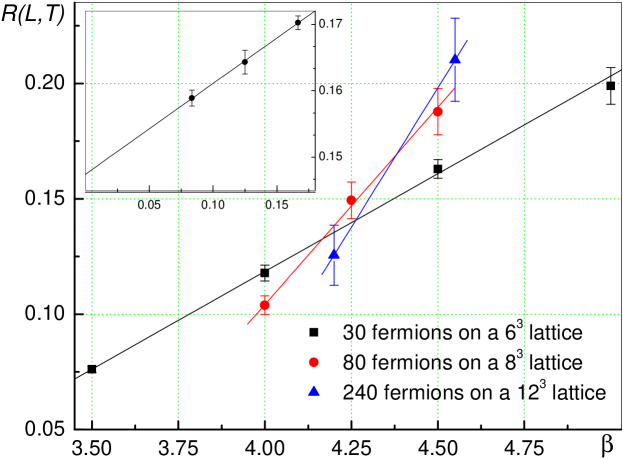
Figure 4: A typical crossing of the $R(L,T)$ curves. The errorbars are $2\sigma$, and solid lines are the linear fits to the MC points. Inset shows the finite-size scaling of the filling factor ($\nu$ vs $1/L$), which yields $\nu=0.148(1)$. From this plot and Eq. (1.1c) one obtains $1/T_{c}(\nu)=4.41(5)/t$

.

Shown in figure 5 is the dependence of the critical temperature on the lattice filling factor. The critical temperature is measured in units of the Fermi energy, as is natural for the unitarity limit. We define the Fermi momentum for a lattice system with filling factor $\nu$ as $k_{F}=(3\pi^{2}\nu)^{1/3}$ and the Fermi energy $\varepsilon_{F}=k_{F}^{2}$, as those of a continuum gas with the same effective mass and number density $n=\nu$.

It is clearly seen that the presence of the lattice suppresses the critical temperature considerably, nearly by a factor of $4$, depending on the filling factor. Strong dependence of $T_{c}$ on $\nu$ is in apparent contradiction with Ref. [24], which claims weak or no $\nu$-dependence. This disagreement might be due to the difference in the single-particle spectra $\varepsilon_{\mathbf{k}}$ used: Ref. [24] employs the parabolic spectrum with spherically symmetric cutoff, while we use the tight-binding dispersion law. Indeed, Eqs. (1.1h)-(1.1i) indicate that a particular choice of $\varepsilon_{\mathbf{k}}$ does influence lattice corrections to $T_{c}$, which may even have different signs for different $\varepsilon_{\mathbf{k}}$.

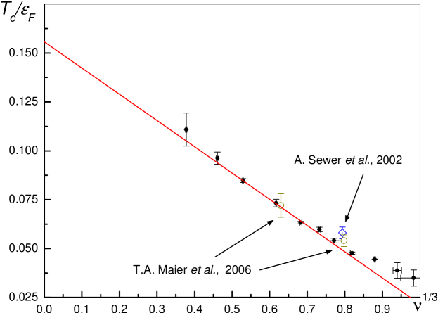
Figure 5: The scaling of the lattice critical temperature with filling factor (circles). $\nu=1$ corresponds to the half filling. The errorbars are one standard deviation. The results of Ref. [42, 43] at quarter filling and $\nu=0.25$ are also shown for a comparison. See the text for discussion.

It is also clear from figure 5 that close to half-filling $T_{c}$ is essentially constant, as expected (see, e.g. [44]). The predicted $\sim\nu^{1/3}$ scaling (1.1j) sets in at about $\nu\approx 0.5$. We thus use a linear fit $T_{c}(\nu)/\varepsilon_{F}(\nu)=T_{c}/\varepsilon_{F}-\mathrm{const}\cdot\nu^{1/3}$ to eliminate lattice corrections in the final result. Such fitting procedure results in the best-fit line given by $0.152(7)-0.13(2)\nu^{1/3}$. We further analyze the fit residues in order to estimate the effect of the sub-leading lattice corrections which are expected to be proportional to $\nu^{2/3}$. As shown in figure 6, such corrections, if any, are smaller than the uncertainty of the $\nu^{1/3}$ fit.

This analysis yields the final result $T_{c}/\varepsilon_{F}=0.152(7)$ for the continuum uniform gas, which is noticeably below the transition temperature in the BEC limit $T_{\mathrm{BEC}}=0.218\varepsilon_{F}$. Various approximate analytical treatments led in the past to $T_{c}$ either above [10, 12, 13, 15], or below [11, 14, 16] $T_{\mathrm{BEC}}$.

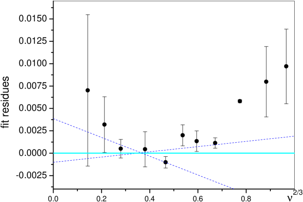
Figure 6: The fit residues for the best-fit line of figure 5, plotted versus $\nu^{2/3}$ (circles). Zero level is shown by the horizontal line, the blue dashed lines are linear fits to the data points for $\nu<0.5$ and $\nu<0.35$, respectively.

Is is instructive to compare our results for $T_{c}$ to other numerical calculations available from the literature. The simulations of Ref. [25] yield $T_{c}=0.05\varepsilon_{F}$, but at the value of the scattering length which has not been determined precisely. This result most probably corresponds to a deep BCS regime, where the transition temperature is exponentially suppressed. Lee and Schäfer [26] report an upper limit $T_{c}<0.14\varepsilon_{F}$, based on a study of the caloric curve of a unitary Fermi gas down to $T/\varepsilon_{F}=0.14$ for filling factors down to $\nu=0.5$. The caloric curve of Ref. [26] shows no signs of divergent heat capacity which would signal the phase transition. This upper limit is consistent with $T_{c}(\nu=0.5)/\varepsilon_{F}\approx 0.054$, see figure 5.

The Seattle group has performed simulations of the caloric curve and condensate fraction, $n_{0}$, of the unitary gas, Ref. [24]. Using “visual inspection” of the caloric curve shape the critical temperature was estimated in Ref. [24] to be $T_{c}=0.22(3)\varepsilon_{F}$. Unfortunately, the authors did not perform the finite-size analysis and $\nu\to 0$ extrapolation. The overall shape of the caloric curve seem to be little affected by the finite volume of the system. This is hardly surprising since even in the thermodynamic limit $E(T)$ and its derivative $\rmd E/\rmd T$ are continuous at the transition point. These properties also make it hard to use non-quantitative measures for reliable estimates of critical parameters from the $E(T)$ curve. On the other hand, the condensate fraction which has singular properties at $T_{c}$ does show sizable finite-size corrections, see figure 1 of Ref. [24]. At this point we note that scaling of the condensate fraction is identical to that for $K(L,T)$. In figure 7 we plot the data of Seattle’s group as $n_{0}L^{1+\eta}$ versus temperature. The intersection of scaled curves turns out to be inconsistent with the estimate for $T_{c}$ derived from the caloric curve inspection.

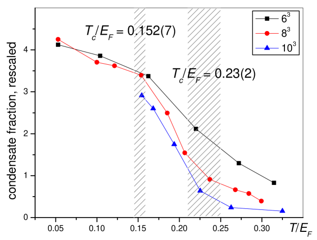
Figure 7: The finite-size scaling of the condensate fraction data from Ref. [24]. Raw data points are rescaled similar to Eq. (1.1a) by the $L^{1+\eta}$ factor. Shaded vertical strips represent results for $T_{c}/\varepsilon_{F}$ of this work and Ref. [24], respectively, solid lines are drawn to guide an eye.

6.2 Thermodynamic functions

The filling factor dependence of thermodynamic quantities is similar to that of $T_{c}$: Figure 8 displays the behaviour of energy and chemical potential along the critical line $T=T_{c}(\nu)$. The extrapolation towards $\nu\to 0$ yields for the continuum gas

$$E/(N\varepsilon_{F})\;=\;0.31(1)~{}~{}~{}~{}~{}~{}~{}~{}~{} (T=T_{c})\;,$$ (1.1a)

$$\mu/\varepsilon_{F}\;=\;0.493(14)~{}~{}~{}~{}~{}~{}~{}~{}~{} (T=T_{c})\;.$$ (1.1b)

The numerical values for other thermodynamic functions at criticality can be easily restored using the formulas of Sec. 5.

Figure 8: Energy (left-hand panel) and chemical potential (right-hand panel) dependence on the filling factor along the critical isotherm $T=T_{c}(\nu)$. Dots are the MC results, dashed lines are the linear fits.

In order to elucidate the thermodynamic behaviour of the unitary gas, we performed simulations for a range of temperatures $T>T_{c}$. Shown in figure 9 are the simulation results for energy and chemical potential for the continuum gas as functions of temperature. Each point was obtained using data analysis similar to that depicted in figure 8. In the high-temperature region we simulated up to $80$ fermions on lattices with up to $32^{3}$ sites. In this region, the condition $\nu\ll 1$ is necessary but not sufficient for extrapolation to the continuum limit, for it is crucial to keep temperature much smaller than the bandwidth: $T\ll 6t$.

As can be seen from figure 9, our results for both energy and chemical potential approach the virial expansion [40] as $T/\varepsilon_{F}\to\infty$. For $T/\varepsilon_{F}\leqslant 0.5$ our data are not far from the curve of Ref. [24]. Though we do not have data points for $T<T_{c}$ there is still a reasonable agreement even at $T_{c}$ with the $T\to 0$ fixed-node MC values [19]. In this region, our results are consistent with a very weak dependence of energy and chemical potential on temperature, and the numeric values of both are consistent with the experimental results [3, 4, 5].

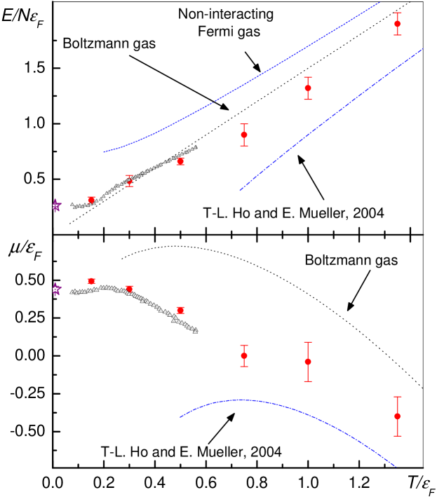
Figure 9: The temperature dependence of the energy per particle (upper panel) and chemical potential (lower panel) of the unitary Fermi gas. Red circles are the MC results, black dotted lines and blue dashed lines correspond to the Boltzmann and non-interacting Fermi gases, respectively, the dot-fashed lines are the asymptotic prediction of Ref. [40] (plus the first virial Fermi correction), black triangles are the MC results of Ref. [24], and the purple stars denote the ground-state fixed-node MC results [19].

Using Eq. (1.1i) and data from figure 9 we deduce the dependence of free energy on temperature, see figure 10. We also use Eq. (1.1j) to make sure that our MC data for energy and chemical potential are consistent with each other.

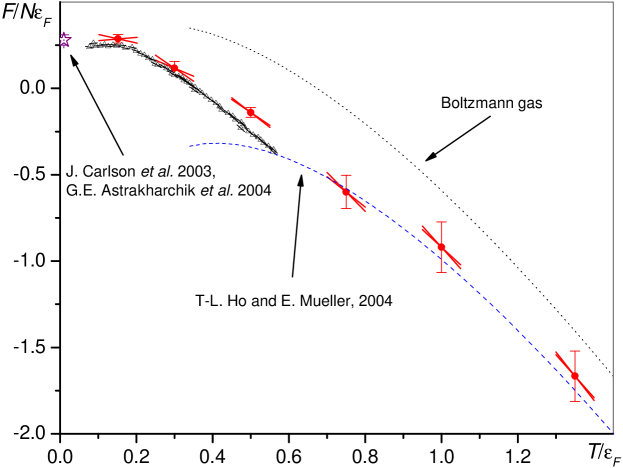
Figure 10: Free energy versus temperature. Red dots are the MC data, and dashes represent the errorbar range for derivative of free energy, calculated via Eq. (1.1j). Black triangles are MC results of Ref. [24], purple star denotes the ground-state fixed-node MC result [19], black dotted line shows the Boltzmann gas curve, and the blue dashed is the asymptotic prediction of Ref. [40].

6.3 Trapped gas

As discussed in Sec. 5.1, the thermodynamic functions for the uniform case can be used for analysis of experimental system within the local density approximation. In this section we report preliminary results of our ongoing study of trapped gas experiments.

It starts with the interpolation procedure which produces continuous functional behaviour for thermodynamic functions, consistent with the discrete set of simulated points. We use a piecewise-cubic ansatz with a smooth crossover to the virial expansion, Eq. (1.1p), for the free energy. Temperature dependence of both energy and entropy are then deduced using numerical integration of Eqs. (1.1x) and (1.1y), respectively.

As the trapped gas is cooled down, the superfluidity first sets in at the centre of the trap, where the density is the highest. Equation (1.1v) can be used to pinpoint this onset temperature: at $T=T_{c}$, $\mu/T=(\mu/\varepsilon_{F}^{0})/(T/\varepsilon_{F}^{0})$, where $\varepsilon_{F}^{0}$ is the Fermi energy of the uniform gas with the density equal to the density at the trap centre. Using $T_{c}/\varepsilon_{F}^{0}=0.152(7)$ and Eq. (1.1b), one obtains $T_{c}/E_{F}=0.20(2)$. We quote here a conservative estimate for the uncertainty, which incorporates both the uncertainty of the critical temperature itself, and a systematic uncertainty which stems from restoring the continuous functional dependence of the chemical potential out of the finite set of the Monte Carlo calculated points with finite errorbars.

Experimentally, the temperature of the strongly interacting Fermi gas is not easily accessible. On the contrary, thermometry of the non-interacting Fermi gases is well established. In the adiabatic ramp experiments one starts from the non-interacting gas at some temperature [in units of Fermi energy] $\left(T/T_{F}\right)^{0}$, and slowly ramps magnetic field towards the Feshbach resonance [6], thus adiabatically connecting the system at unitarity to a non-interacting one. Assuming the entropy conservation during the magnetic field ramp, equation (1.1y) can be employed for the thermometry of the interacting gas: by matching the entropy of a non-interacting gas at the temperature $\left(T/T_{F}\right)^{0}$ with the entropy calculated via Eq. (1.1y) one relates the initial temperature (before the magnetic field ramp) to the final temperature (after the ramp). We find that the onset of the superfluidity corresponds to $\left(T/T_{F}\right)^{0}=0.12\pm 0.02$ (again, we quote here the most conservative estimate for the errorbar). This value seems to be somewhat lower than the value suggested by the experimental results [6]. Nevertheless, given the level of the noise in figure 4 of Ref. [6] the consistency is reasonable.

An alternative thermometry can be build on recent advances in the experimental technique [3, 4] which made it possible to directly image the in situ density profiles of the interacting system. Such density profiles can be directly fit to Eq. (1.1t), which gives the shape of the cloud depending on $\mu/T$ and $T/E_{F}$. By relating the chemical potential to the temperature using Eq. (1.1v), one is left with only one fitting parameter, $T/E_{F}$ (apart from a trivial fitting parameter $z_{0}$ which accounts for the overall shift of the cloud image off the trap centre).

As an illustrative example of such procedure we have analyzed the experimental density profiles measured by the Rice’s group [4], as depicted in figure 11. From this analysis we deduce the upper bound for the temperature in the experiments [4] $T<0.1E_{F}$, which is consistent with the results of the measurements of the condensate fraction [2]. Since in the experiments [2, 4] the gas is very degenerate, one is able to put an upper limit on temperature only.

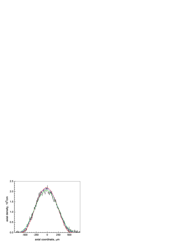
Figure 11: Axial density density profiles: experimental data (dots) is from the data contained in figure 3 of [4]. The full red line is calculated via Eq. (1.1u)–(1.1v) with $T/E_{F}=0.03$ (correspondingly, $T/\varepsilon_{F}^{(0)}=0.02$), dashed blue line corresponds to $T/E_{F}=0.16$ ($T/\varepsilon_{F}^{(0)}=0.1$), and dot-dashed green line is for $T/E_{F}=0.22$ ($T/\varepsilon_{F}^{(0)}=0.16$). In both cases we allowed for a horizontal displacement of a whole curve in the range of $|z_{0}|<20\mu$m. See the text for discussion.

Note that if the temperature is known from, e.g. the adiabatic ramp experiments, Eqs. (1.1t)-(1.1v) must reproduce the cloud shape without free parameters (apart from $z_{0}$).

7 Conclusions

We have developed a worm-type scheme within the systematic-error-free determinant diagrammatic Monte Carlo approach for lattice fermions. We applied it to the Hubbard model with attractive interaction and equal number of spin-up and spin-down particles. At finite densities, the model describes ultracold atoms in optical lattice. In the limit of vanishing filling factor, $\nu\to 0$, and fine-tuned (to the resonance in the two-particle $s$-wave channel) on-site attraction, a universal regime sets in, which is identical to the BCS-BEC crossover in the continuous space. In the present work, we confined ourselves to a special value of the on-site interaction, $U=U_{*}\approx-7.915t$, corresponding to the divergent $s$-scattering length. At $U=U_{*}$ and $\nu\to 0$, the system reproduces the unitary point of the BCS-BEC crossover. The unitary regime is scale-invariant: all thermodynamic potentials are expressed in terms of dimensionless scaling functions of the dimensionless ratio $T/\varepsilon_{F}$ (temperature in units of Fermi energy). We obtained these scaling functions by extrapolating results for the Hubbard model to $\nu\to 0$. For the critical temperature of the superfluid-normal transition in the uniform case we found $T_{c}/\varepsilon_{F}=0.152(7)$. Our results form a basis for an unbiased thermometry of trapped fermionic gases in the unitary regime: In particular, we found (within the local density approximation) that for the parabolic confinement, the critical temperature in units of the characteristic trap energy $E_{F}$ is $T/E_{F}=0.20(2)$. For the experimentally relevant case of an isentropic conversion of a gas from the non-interacting regime to the unitary regime we find that the onset of the superfluidity corresponds to the initial temperature (before the magnetic field ramp) $\left(T/T_{F}\right)^{0}=0.12\pm 0.02$, which is reasonably consistent with the experimental result [6], to within the experimental noise.

Appendix A Updating procedures

The generic diagrammatic MC rules for constructing updates are as follows [45]. Let an update $\mathcal{B}$ transform a diagram $\mathcal{D}(\mathcal{S}_{p})$ into diagram $\mathcal{D}(\mathcal{S}^{\prime}_{q})$. Here configurations $\mathcal{S}_{p}$ and $\mathcal{S}^{\prime}_{q}$ may have different order and may or may not feature the “worm” two-point vertices. The update $\mathcal{B}$ involves two steps. First, a modification of the configuration is proposed, with some probability density $W(\mathcal{S}_{p}\to\mathcal{S}^{\prime}_{q})$ for new continuous/discrete variables. There are no strict requirements fixing the form of $W(\mathcal{S}_{p}\to\mathcal{S}^{\prime}_{q})$, it should rather be chosen on physical grounds to maximize the efficiency of the algorithm, and be simple enough to allow analytical evaluation of the normalization integral. Then, the update is either accepted, with probability $P_{\mathcal{S}_{p}\to\mathcal{S}^{\prime}_{q}}$, or rejected. The complimentary update $\mathcal{C}$, which transforms $\mathcal{D}(\mathcal{S}^{\prime}_{q})$ into $\mathcal{D}(\mathcal{S}_{q})$ proposes the modification with the probability density $W(\mathcal{S}_{p}\leftarrow\mathcal{S}^{\prime}_{q})$, which, in principle, may differ from $W(\mathcal{S}_{p}\to\mathcal{S}^{\prime}_{q})$, and is accepted with the probability $P_{\mathcal{S}_{p}\leftarrow\mathcal{S}^{\prime}_{q}}$. For a pair of updates $\mathcal{B}$ and $\mathcal{C}$ to be balanced, the acceptance probabilities must obey the Metropolis relations [45]

$$P_{\mathcal{S}_{p}\to\mathcal{S}^{\prime}_{q}} =\min(1,\mathcal{R}),$$ (1.1a)

$$P_{\mathcal{S}_{p}\leftarrow\mathcal{S}^{\prime}_{q}} =\min(1,1/\mathcal{R})$$ (1.1b)

where $\mathcal{R}$ is a solution of the detailed-balance equation

$$\mathcal{R}W(\mathcal{S}_{p}\to\mathcal{S}^{\prime}_{q})\mathcal{D}(\mathcal{S}_{p})=W(\mathcal{S}_{p}\leftarrow\mathcal{S}^{\prime}_{q})\mathcal{D}(\mathcal{S}^{\prime}_{q}).$$ (1.1c)

If the probabilities of selecting updates $\mathcal{B}$ and $\mathcal{C}$ are not equal, they must also be included into the definition of $W(\mathcal{S}_{p}\to\mathcal{S}^{\prime}_{q})$ and $W(\mathcal{S}_{p}\leftarrow\mathcal{S}^{\prime}_{q})$, respectively.

A.1 The “Diagonal” updating scheme

The minimal ergodic set of updates, as suggested in [22, 30], consists of just one pair of “diagonal” updates which increase/decrease the number of vertices in a configuration by one: in the forward update one adds a vertex at randomly selected point in the $L^{3}\times\beta$ hypercube; in the reverse update one removes a random vertex from the configuration. In the simplest version, the probability density for selecting a point is uniform, i.e. one selects a particular lattice site with the probability $p(\mathbf{x}_{\mathrm{new}})=L^{-d}$, and a temporal position with the probability density $w(\tau_{\mathrm{new}})=\beta^{-1}$. A vertex to be removed is selected at random out of $p$ vertices present in the configuration. Hence the Metropolis acceptance ratio function (1.1c) is given by

$$\mathcal{R}_{\mathrm{add}}=\left|\frac{\det\mathbf{A}(\mathcal{S}_{p+1})}{\det\mathbf{A}(\mathcal{S}_{p})}\right|^{2}\frac{(-U)\beta L^{d}}{p+1}\;.$$ (1.1d)

Here $\mathcal{S}_{p+1}=(\mathbf{x}_{\mathrm{new}},\tau_{\mathrm{new}})\cup\mathcal{S}_{p}$ is the configuration with an extra vertex $(\mathbf{x}_{\mathrm{new}},\tau_{\mathrm{new}})$. The acceptance ratio to remove a vertex is

$$\mathcal{R}_{\mathrm{rem}}=\left|\frac{\det\mathbf{A}(\mathcal{S}_{p-1})}{\det\mathbf{A}(\mathcal{S}_{p})}\right|^{2}\frac{p}{(-U)\beta L^{d}}\;.$$ (1.1e)

A.2 Worm-type updating scheme

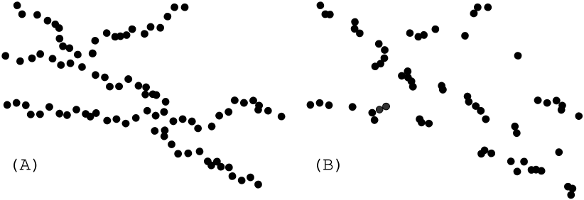
Figure 12: Multi-ladder diagrams in deep BEC regime (A), and close to unitarity (B).

The diagonal updating scheme described in the previous section is highly inefficient in the dilute regime—the regime we are mostly interested in. To assess the efficiency of the “diagonal” scheme consider first a low-density gas in the deep BEC regime. In this limit, all fermions are paired into composite bosons (apart from exponentially rare fluctuations). Inter-boson interactions occur only via rare collisions. In the diagrammatic language, the existence of compact composite bosons is reflected by the fact that the dominant diagrams are the multi-ladder ones (see figure 12A), with the typical $\mathbf{x}$-span of each ladder being of the order of $L$, and the typical $\tau$-span of the order of $\beta$. Each ladder of such a diagram in fact mimics a world line of a composite boson.

The analogy between ladder parts of multi-ladder diagrams and world lines of composite bosons helps elucidating the structure of typical diagrams at resonance. Indeed, at the two-particle resonance composite bosons exist only virtually, but at the same time the energy cost of creating a boson is zero. Thus, multi-ladder diagrams still dominate, but the $\mathbf{x}$- and $\tau$-span of individual ladders becomes finite and related to the inter-particle distance, see figure 12B. Resonant ladders also become more “dilute” since the average distance between vertices diverges, but they still contain many vertices since the resonance formation involves distances much smaller than $\nu^{-1/3}$.

Proposing diagrams which disregard the nature of the resonant interaction results in small acceptance ratios. To significantly reduce this type of slowing down, we resort to a worm-type updating scheme which allows one to, loosely speaking, directly “draw” the multi-ladder diagrams.

A.2.1 Worm creation/annihilation updates

These updates are the necessary ingredient of the worm-type scheme, since they switch between the diagonal (1.1c) and off-diagonal (1.1i) diagrams. These updates transform diagrams as follows:

$$\mathfrak{S}^{(Z)}\ni\mathcal{S}_{p}=\{\dots,\,(\mathbf{x}_{1},\tau_{1}),\,\dots\}\leftrightarrows$$ (1.1f)

$$\{\dots,\,(\mathbf{x}_{1},\tau_{1}),\,P(\mathbf{x},\tau),\,P^{\dagger}(\mathbf{x}^{\prime},\tau^{\prime}),\,\dots\}=\widetilde{\mathcal{S}}_{p}\in\mathfrak{S}^{(G)}\;.$$ (1.1g)

To create a pair of two-point vertices $P(\mathbf{x},\tau)$ and $P^{\dagger}(\mathbf{x}^{\prime},\tau^{\prime})$, one first selects $\mathbf{x}$ and $\tau$ uniformly over the spatial lattice and $(0,\beta)$ interval, respectively. One then selects $\mathbf{x}^{\prime}$ among the lattice sites in the spatial cube with the edge length $l$ centered around $\mathbf{x}$ with equal probabilities, and selects $\tau$ uniformly on the interval $(\tau-\Delta\tau/2,\tau+\Delta\tau/2)$. The values of $l$ and $\Delta\tau$ are arbitrary. The overall probability density is thus given by:

$$W(\mathcal{S}_{p}\to\widetilde{\mathcal{S}}_{p})\;=\;\frac{1}{\beta L^{d}}\,\frac{1}{\Delta\tau l^{d}}\;.$$ (1.1h)

The reverse update attempts to remove $P(\mathbf{x},\tau)$ and $P(\mathbf{x}^{\prime},\tau^{\prime})$ provided $|\mathbf{x}_{\alpha}-\mathbf{x}^{\prime}_{\alpha}|<l/2$ ($\alpha=1,2,3$) and $|\tau-\tau^{\prime}|<\Delta\tau/2$, as prescribed by the balance requirement.

The solution to the detailed balance equation (1.1c) then reads:

$$\mathcal{R}=\left|\frac{\det\mathbf{A}(\widetilde{\mathcal{S}}_{p})}{\det\mathbf{A}(\mathcal{S}_{p})}\right|^{2}\beta L^{d}\Delta\tau l^{d}\zeta\;.$$ (1.1i)

In order to maximize the efficiency of the numerical scheme, it is advantageous to have the acceptance probabilities (1.1a)-(1.1b) to be of the order unity. On the other hand, the explicit macroscopically large factors in the right-hand side of Eq. (1.1i) render the acceptance probabilities macroscopic. The use of the extra weighting factor $\zeta$ is now clear: by choosing $1/\zeta=\beta L^{d}\Delta\tau l^{d}/\widetilde{\zeta}$ one removes undesired factors from the right-hand side of Eq. (1.1i). The remaining freedom of choosing $\widetilde{\zeta}$ has to be employed to further fine-tune the acceptance probabilities. The required values of $\widetilde{\zeta}$ are typically of the order of unity.

A.2.2 Adding/removing vertices within the worm framework

These updates are central for the method since they change the diagram order. The main idea of these updates is: given a pair of “worm” two-point vertices $P$ and $P^{\dagger}$, use, say, $P^{\dagger}(\mathbf{x},\tau)$ as a tip of a magic pen to add or remove vertices from the diagram (note that it suffices to use either $P$ or $P^{\dagger}$ as a dynamical variable, the choice being only a matter of taste):

$$\widetilde{\mathcal{S}}_{p}=\{\dots,\,(\mathbf{x}_{1},\tau_{1}),\,P^{\dagger}(\mathbf{x},\tau),\,\dots\}\leftrightarrows$$ (1.1j)

$$\{\dots,\,(\mathbf{x}_{1},\tau_{1}),\,(\mathbf{x},\tau),\,P^{\dagger}(\mathbf{x}_{\mathrm{new}},\tau_{\mathrm{new}}),\,\dots\}=\widetilde{\mathcal{S}}^{\prime}_{p+1}\;.$$ (1.1k)

We have employed two versions of these updates.

High-density version

In the most simple yet useful version of a forward update, one selects $\tau_{\mathrm{new}}$ and $\mathbf{x}_{\mathrm{new}}$ uniformly in the interval $(\tau-\Delta\tau/2,\tau+\Delta\tau/2)$, and the spatial cube of the edge length $l$ centered at $\mathbf{x}$, correspondingly. In the reverse update one selects a vertex to be removed at random out of $m$ choices, where $m$ is the number of vertices $(\mathbf{x}_{i},\tau_{i})$ such that $|(\mathbf{x}_{i})_{\alpha}-(\mathbf{x}_{\mathrm{new}})_{\alpha}|<l/2$ and $|\tau_{i}-\tau_{\mathrm{new}}|<\Delta\tau/2$. The solution to the detailed balance equation then reads

$$\mathcal{R}\;=\;\left|\frac{\det\mathbf{A}(\widetilde{\mathcal{S}}_{p+1}^{\prime})}{\det\mathbf{A}(\widetilde{\mathcal{S}}_{p})}\right|^{2}\,\frac{(-U)\Delta\tau l^{d}}{m}\;.$$ (1.1l)

Low-density version

The strategy just described works well close to half-filling. In the low-density regime the multi-ladder diagrams dominate and the above scheme is not optimal for a number of reasons: (i) it does not respect the diagram structure which should feature (at least locally) well-defined vertex chains; (ii) the probability density according to which the value of $\tau_{\mathrm{new}}$ is proposed should favour shifting $P^{\dagger}$ towards smaller $\tau$-s. To see this, consider two particles in vacuum: the matrix elements of $P^{\dagger}(\mathbf{x},\tau_{1})P(\mathbf{x},\tau_{2})$ simply equal zero for $\tau_{2}<\tau_{1}$.]; (iii) both large and small values of $\delta\tau=\tau-\tau_{\mathrm{new}}$ have to be accounted for. Consider two fermions in vacuum again. The local probability density for a shift of length $\delta\tau$ and $\mathbf{x}_{\mathrm{new}}=\mathbf{x}$ is proportional to the free diffusion propagator: $w(\delta\tau)\propto\delta\tau^{-3/2}$, which is singular as $\delta\tau\to 0$. However, the mean value of $\delta\tau$ for this distribution, $\int w(\delta\tau)\delta\tau\,\rmd(\delta\tau)$, diverges at the upper limit. These properties of resonant ladders are ignored when shifts are proposed uniformly over some $\pm\Delta\tau$ interval.

The requirements (ii) and (iii) are best met if, when adding a vertex, a new position of $P^{\dagger}$ is proposed according to the probability density [cf. Eq. (1.1k)]

$$w(\mathbf{x}_{\mathrm{new}}-\mathbf{x};\delta\tau)\propto\left\{\begin{array}[]{ll}\left|G^{(0)}(\mathbf{x}-\mathbf{x}_{\mathrm{new}},\,\tau-\tau_{\mathrm{new}})\right|^{2},&\mathrm{if~{}~{}}\tau_{\mathrm{new}}>\tau\;,\\ 0,&\mathrm{otherwise.}\end{array}\right.$$ (1.1m)

Since the free single-particle propagator is known only numerically, we use Eq. (1.1m) on a uniform mesh with some step $\sigma$: $\delta\tau_{j}=\sigma j$. That is, we tabulate the values $w_{j}=w(\mathbf{y};\delta\tau_{j})$ prior to the start of computations; we then select $\mathbf{y}$ and $\delta\tau_{j}$ according to the (normalized) distribution $w(\mathbf{y};\delta\tau_{j})$. The proposed new position of $P^{\dagger}$ is then chosen as $\mathbf{x}_{\mathrm{new}}=\mathbf{x}+\mathbf{y}$, and $\tau_{\mathrm{new}}=\tau+\delta\tau_{j}+\Delta$, where $\Delta$ is uniform over the interval $[-\sigma/2,\sigma/2]$. We find that $\sigma\sim 1/5U$ produces good results.

In order to meet the requirement (i), the notion of the closest—in terms of a certain distance—neighboring vertex is introduced: the reverse update $\mathcal{S}^{\prime}_{p+1}\to\mathcal{S}_{p}$ deterministically deletes the closest neighbor of $P^{\dagger}$. The detailed balance than requires that the forward update should be automatically rejected whenever $(\mathbf{x},\tau)$ is not the closest neighbor of $P^{\dagger}(\mathbf{x}_{\mathrm{new}},\tau_{\mathrm{new}})$, cf. Eq. (1.1k). We define the distance between vertices using a simple Euclidean norm $\|(\mathbf{x},\tau)-(\mathbf{x}_{\mathrm{new}},\tau_{\mathrm{new}})\|=(\mathbf{x}-\mathbf{x}_{\mathrm{new}})^{2}/L^{2}+(\tau-\tau_{\mathrm{new}})^{2}/\beta^{2}$.

The acceptance ratio function (1.1c) is then

$$\mathcal{R}=\left|\frac{\det\mathbf{A}(\widetilde{\mathcal{S}}_{p+1}^{\prime})}{\det\mathbf{A}(\widetilde{\mathcal{S}}_{p})}\right|^{2}\frac{(-U)\sigma}{w_{j}}\;,$$ (1.1n)

where $w_{j}$ is given by Eq. (1.1m).

The scheme (1.1n) in the dilute regime typically yields a an order of magnitude gain in efficiency, as compared to the scheme (1.1l).

A.2.3 Shifting the worm two-point vertices

Clearly, the scheme (1.1n) should be supplemented by an update which allows for an easy change of the closest neighbor. The following update performs the task:

$$\widetilde{\mathcal{S}}_{p}\;=\;\{\dots,\,P(\mathbf{x},\tau),\,\dots\}\leftrightarrows\{\dots,\,P(\mathbf{x}^{\prime},\tau^{\prime}),\,\dots\}\;=\;\widetilde{\mathcal{S}}^{\prime}_{p}\;.$$ (1.1o)

We select $\mathbf{x}^{\prime}$ among the nearest neighbors of the lattice site $\mathbf{x}$ with equal probabilities and $\tau^{\prime}$ uniformly in some interval around $\tau$.

This update is self-balanced, and the acceptance ratio function $\mathcal{R}$ is simply

$$\mathcal{R}\;=\;\left|\frac{\det\mathbf{A}(\widetilde{\mathcal{S}}_{p})}{\det\mathbf{A}(\widetilde{\mathcal{S}}^{\prime}_{p})}\right|^{2}\;.$$ (1.1p)

References

References

- [1] Dieckmann K, Stan C A, Gupta S , Hadzibabic Z, Schunck C H and Ketterle W 2002 Phys. Rev. Lett.89 203201Regal C A, Ticknor C, Bohn J L and Jin D S 2003 Nature 424 47Bourdel T, Cubizolles J, Khaykovich L, Magalhães K M F, Kokkelmans S J J M F, Shlyapnikov G V and Salomon C 2003 Phys. Rev. Lett.91 020402Strecker K E, Partridge G B and Hulet R G 2003 Phys. Rev. Lett.91 080406Cubizolles J, Bourdel T, Kokkelmans S J J M F, Shlyapnikov G V and Salomon C 2003 Phys. Rev. Lett.91 240401Jochim S, Bartenstein M, Altmeyer A, Hendl G, Chin C, Hecker Denschlag J and Grimm R 2003 Phys. Rev. Lett.91 240402 Zwierlein M W, Stan C A, Schunck C H, Raupach S M F, Gupta S, Hadzibabic Z and Ketterle W 2003 Phys. Rev. Lett.91 250401Greiner M, Regal C A and Jin D S 2003 Nature 426 537Jochim S, Bartenstein M, Altmeyer A, Hendl G, Riedl S, Chin C, Hecker Denschlag J and Grimm R 2003 Science 302 2101Regal C A, Greiner M and Jin D S 2004 Phys. Rev. Lett.92 083201Zwierlein M W, Stan C A, Schunck C H, Raupach S M F, Kerman A J and Ketterle W 2004 Phys. Rev. Lett.92 120403Kinast J, Hemmer S L, Gehm M E, Turlapov A and Thomas J E 2004 Phys. Rev. Lett.92 150402Bartenstein M, Altmeyer A, Riedl S, Jochim S, Chin C, Hecker Denschlag J and Grimm R 2004 Phys. Rev. Lett.92 203201 Chin C, Bartenstein M, Altmeyer A, Riedl S, Jochim S, Hecker Denschlag J and Grimm R 2004 Science 305 1128Zwierlein M W, Abo-Shaeer J R, Schirotzek A, Schunck C H and Ketterle W 2005 Nature 435 1047
- [2] Partridge G B, Strecker K E, Kamar R I, Jack M W and Hulet R G 2005 Phys. Rev. Lett.. 95 020404
- [3] Bartenstein M, Altmeyer A, Riedl S, Jochim S, Chin C, Hecker Denschlag J and Grimm R Phys. Rev. Lett.2004 92 120401
- [4] Partridge G B, Li W, Kamar R I, Liao Y-A and Hulet R G 2006 Science 311 503
- [5] O’Hara K M, Hemmer S L, Gehm M E, Granade S R and Thomas J E 2002 Science 298 2179Bourdel T, Khaykovich L, Cubizolles J, Zhang J, Chevy F, Teichmann M, Tarruell L, Kokkelmans S J J M F and Salomon C 2004 Phys. Rev. Lett.93 050401Kinast J, Turlapov F, Thomas J E, Chen Q, Stajic J and Levin K 2005 Science 307 1296
- [6] Regal C A, Greiner M and Jin D S 2004 Phys. Rev. Lett.92 040403
- [7] Modugno G, Ferlaino F, Heidemann R, Roati G and Inguscio M 2003 Phys. Rev.A 68 011601(R) Köhl M, Moritz H, Stöferle T, Günter K and Esslinger T 2005 Phys. Rev. Lett.94 080403Moritz H, Stöferle T, Günter K, Köhl M and Esslinger T 2005 Phys. Rev. Lett.94 210401Stöferle T, Moritz H, Günter K, Köhl M and Esslinger T 2006 Phys. Rev. Lett.96 030401Köhl M, Günter K, Stöferle T, Moritz H and Esslinger T 2006 J. Phys. B: At. Mol. Opt. Phys. 39 S47
- [8] Heiselberg H and Hjorth-Jensen M 2000 Phys. Rep. 328 237 Heiselberg H 2001 Phys. Rev.A 63 043606 Baker G A, Jr 1999, Phys. Rev.C 60 054311
- [9] Eagles D R 1969 Phys. Rev.186 456 Legett A J 1980, in Modern Trends in the Theory of Condensed Matter (Lecture notes in physics vol 115) ed Pekalski A and Przystawa R (Berlin: Springer-Verlag)
- [10] Nozières P and Schmitt-Rink S 1985 J. Low Temp. Phys. 59 195
- [11] Haussmann R 1994 Phys. Rev.B 49 12975
- [12] Randeria M 1995, in Bose-Einstein Condensation, ed Griffin A et al(Cambridge: Cambridge University Press)
- [13] Holland M, Kokkelmans S J J M F, Chiofalo M L and Walser R 2001 Phys. Rev. Lett.87 120406Timmermans E, Furuya K, Milloni PW and Kerman A K 2001 Phys. Lett.A 285 228
- [14] Ohashi Y and Griffin A 2002 Phys. Rev. Lett.89 103402
- [15] Perali A, Pieri P, Pisani L and Strinati G C 2004 Phys. Rev. Lett.92 220404
- [16] Liu X-J and Hu H 2005 Phys. Rev.A 72 063613
- [17] Binder K and Landau D P 2000 A Guide to Monte Carlo Simulations in Statistical Physics (Cambridge: Cambridge University Press)
- [18] Troyer M and Wiese U-J 2005 Phys. Rev. Lett.94 170201
- [19] Carlson J, Chang S-Y, Pandharipande V R and Schmidt K E 2003 Phys. Rev. Lett.91 050401 Chang S-Y, Pandharipande V R, Carlson J and Schmidt K E 2004 Phys. Rev.A 70 043602 Astrakharchik G E Boronat J, Casulleras J and Giorgini S 2004 Phys. Rev. Lett.93 200404 Astrakharchik G E Boronat J, Casulleras J and Giorgini S 2005 Phys. Rev. Lett.95 230405
- [20] Scalapino D J and Sugar R L 1981 Phys. Rev. Lett.46 519Blankenbecler R, Scalapino D J and Sugar R L 1981 Phys. Rev.D 24 2278
- [21] Rombouts S M A, Heide K and Jachowicz N 1999 Phys. Rev. Lett.82 4155
- [22] Rubtsov A N 2003 Preprint cond-mat/0302228Rubtsov A N and Lichtenstein A I 2004 Pis’ma v JETP 80 67Rubtsov A N, Savkin V V and Lichtenstein A I 2004 Preprint cond-mat/0411344
- [23] Chen J-W and Kaplan D B 2004 Phys. Rev. Lett.92 257002
- [24] Bulgac A, Drut J E and Magierski P 2006 Phys. Rev. Lett.96 090404
- [25] Wingate M 2005 Preprint cond-mat/0502372
- [26] Lee D T and Schäfer T 2005 Preprint nucl-th/0509018
- [27] Burovski E, Prokof’ev N, Svistunov B and Troyer M 2006 Phys. Rev. Lett.96 160402
- [28] Fetter A L and Walecka J D 1971 Quantum Theory of Many-particle Systems (New York: McGraw-Hill)
- [29] Landau L D and Lifshitz E M 1980 Statistical Physics vol 2 (New York: Pergamon Press)
- [30] Burovski E, Prokof’ev N and Svistunov B 2004 Phys. Rev.B 70 193101(R)
- [31] Prokof’ev N V and Svistunov B V 1998 Phys. Rev. Lett.81 2514
- [32] Mishchenko A, Prokof’ev N, Sakamoto A and Svistunov B 2000 Phys. Rev.B 62 6317
- [33] Metropolis N, Rosenbluth A W, Rosenbluth M N, Teller A M and Teller E 1953 J. Chem. Phys.21 1087
- [34] Prokof’ev N V, Svistunov B V and Tupitsyn I S 1998 Phys. Lett.A 238 253
- [35] see, e.g. Fisher M E 1983, in Lecture Notes in Physics 186 (Springer-Verlag, 1983).
- [36] Binder K 1981 Phys. Rev. Lett.47 693
- [37] see, e.g. Guida R and Zinn-Justin J 1998 J. Phys. A: Math. Gen.31 8103
- [38] Ho T -L 2004 Phys. Rev. Lett.92 090402
- [39] Landau L D and Lifshitz E M 1980 Statistical Physics vol 1 (New York: Pergamon Press)
- [40] Ho T-L and Mueller E J 2004 Phys. Rev. Lett.92 160404
- [41] Husslein T, Fettes W and Morgenstern I 1997 Int. J. Mod. Phys. C8 397
- [42] Sewer A, Beck H and Zotos X 2002 Phys. Rev.B 66 140504
- [43] Maier T A et al, DCA/QMC, unpublished
- [44] Micnas R, Ranninger J and Robaszkiewicz S 1990 Rev. Mod. Phys.62 113
- [45] Prokof’ev N V, Svistunov B V and Tupitsyn I S 1998 Sov. Phys.–JETP 87 310