Spinon excitations in the XX chain: spectra, transition rates, observability

Abstract

The exact one-to-one mapping between (spinless) Jordan-Wigner lattice fermions and (spin-1/2) spinons is established for all eigenstates of the one-dimensional $s=1/2$ $XX$ model on a lattice with an even or odd number $N$ of lattice sites and periodic boundary conditions. Exact product formulas for the transition rates derived via Bethe ansatz are used to calculate asymptotic expressions of the 2-spinon and 4-spinon parts (for large even $N$) as well as of the 1-spinon and 3-spinon parts (for large odd $N$) of the dynamic spin structure factors. The observability of these spectral contributions is assessed for finite $N$ and for $N\to\infty$.

1 Introduction

The exact solution of the $XX$ model for exchange-coupled electron spins on a one-dimensional lattice was first demonstrated more than 40 years ago [1, 2]. Among all integrable quantum many-body systems, the $XX$ model is perhaps the one investigated most thoroughly [3, 4, 5, 6, 7, 8, 9, 10, 11, 12, 13, 14].

The $XX$ interaction between nearest-neighbor spins with $s=1/2$ along a chain of $N$ sites is described by the Hamiltonian

$$\mathcal{H}_{XX}=\sum_{\ell=1}^{N}[S_{\ell}^{x}S_{\ell+1}^{x}+S_{\ell}^{y}S_{\ell+1}^{y}].$$ (1.1)

The exact Jordan-Wigner mapping of this system onto a system of free, spinless lattice fermions has been at the root of most advances reported for this model. The many nontrivial properties of the $XX$ model are accounted for by the non-local functional relation between spin operators and fermion operators.

In spite of steady progress on the $XX$ model reported since 1961, some questions of interest have resisted satisfactory answers. The objective of this paper is to communicate significant advances on two such issues: (i) We establish an exact one-to-one mapping between the fermion composition and the spinon composition of all $XX$ eigenstates, thus linking the computationally convenient fermion quasiparticles to the physically relevant spinon quasiparticles on a rigorous basis. (ii) We use the exact product formulas for transition rates previously derived in the framework of the Bethe ansatz [15] to calculate exact and asymptotic expressions of the $m$-spinon dynamic spin structure factors at $T=0$ with $m=2,4$ for even $N$ and $m=1,3$ for odd $N$. The nature of the results raises questions regarding the observability of specific sets of $m$-spinon excitations and suggests that we distinguish a mesoscopic regime $(N\sim 10^{2}-10^{3})$ from a macroscopic regime $(N\to\infty)$.

The exclusion statistics of the fermion and spinon quasiparticles as well as the mapping between them is described in Sec. 2. The properties of $m$-spinon dynamic structure factors are discussed in Sec. 3 and the observability of $m$-spinon excitations in Sec. 4.

2 Fermions versus spinons

It is desirable to carry out calculations for the $XX$ model using the fermions because they are free and to interpret all spectral properties in terms of the (interacting) spinons because the spinon vacuum, unlike the fermion vacuum, is at the bottom of the spectrum. Hence to calculate the $m$-spinon parts of the $T=0$ dynamic spin structure factors from exact transition rate formulas based on fermion momenta, we must understand in detail how the fermion and spinon quasiparticles are related.

We consider the $XX$ model for even $N$ or odd $N$ and with periodic boundary conditions. The Jordan-Wigner transform followed by a Fourier transform to the reciprocal lattice converts Hamiltonian (1.1) into

$$\mathcal{H}_{XX}=\sum_{\{k_{i}\}}\cos k_{i}\,c_{k_{i}}^{\dagger}c_{k_{i}}.$$ (2.1)

Here $c_{k}^{\dagger},c_{k}$ are fermion creation and annihilation operators. The sum $\{k_{i}\}$ is over the allowed fermion momenta:

$$k_{i}=\frac{\pi}{N}\,\bar{m}_{i},\quad\bar{m}_{i}\in\left\{\begin{tabular}[]{ll}${\displaystyle\{1,3,\ldots,2N-1\}}$&(even $N_{f}$)\\ ${\displaystyle\{0,2,\ldots,2N-2\}}$&(odd $N_{f}$)\end{tabular}\right..$$ (2.2)

The number of fermions varies over the range $0\leq N_{f}\leq N$.

2.1 Exclusion statistics

The number of eigenstates composed of $N_{f}$ fermions is described by the combinatorial formula

$$W_{f}(N_{f})=\left(\begin{tabular}[]{c}$d+N_{f}-1$\\ $N_{f}$\end{tabular}\right),\quad d=N-N_{f}+1.$$ (2.3)

The number of (spinless) fermions present in an eigenstate is related to the quantum number $S_{T}^{z}$ ($z$-component of the total spin) of that state as follows:

$$N_{f}=\frac{N}{2}-S_{T}^{z}.$$ (2.4)

The ground state of $\mathcal{H}_{XX}$ is non-degenerate for even $N$. It contains $N_{f}=N/2$ fermions. This state is reconfigured as the vacuum for spinon quasiparticles. The (spin-1/2) spinons obey semionic exclusion statistics. The number of eigenstates composed of $n_{+}$ spinons with spin up and $n_{-}$ spinons with spin down is described by Haldane’s generalization of (2.3) to fractional statistics [16]:

$$W(n_{+},n_{-})=\prod_{\sigma=\pm}\left(\begin{tabular}[]{c}$d_{\sigma}+n_{\sigma}-1$\\ $n_{\sigma}$\end{tabular}\right),$$ (2.5)

$$d_{\sigma}=\frac{1}{2}(N+1)-\frac{1}{2}\sum_{\sigma^{\prime}}(n_{\sigma^{\prime}}-\delta_{\sigma\sigma^{\prime}}).$$ (2.6)

The total number of spinons,

$$n_{+}+n_{-}=N_{s},$$ (2.7)

is restricted to the values $N_{s}=0,2,\ldots,N$ for even $N$ and to the values $N_{s}=1,3,\ldots,N$ for odd $N$. Eigenstates with a fixed number of spinons may contain different numbers of fermions and vice versa. However, from (2.4) we infer

$$n_{+}-n_{-}=N-2N_{f}.$$ (2.8)

Knowledge of $n_{+}$ and $n_{-}$ for a given eigenstate is thus equivalent to knowledge of $N_{s}$ and $N_{f}$.

In Table 1 we list the numbers of eigenstates for $N=6$ (left) and $N=7$ (right) with given $N_{s}$ in the spinon representation and given $N_{f}$ in the fermion representation.

Table 1: Number $W(n_{+},n_{-})$ of eigenstates with $N_{s}=n_{+}+n_{-}$ spinons and (in a different representation) $N_{f}=N/2-(n_{+}-n_{-})/2$ fermions for $\mathcal{H}_{XX}$ with $N=6$ (left) and $N=7$ (right). Subtotals (2.9) and (2.10) are found in the last column and row, respectively.

$N_{f}\backslash N_{s}$ 0 2 4 6 $0$ – – – 1 1 $1$ – – 5 1 6 $2$ – 6 8 1 15 $3$ 1 9 9 1 20 $4$ – 6 8 1 15 $5$ – – 5 1 6 $6$ – – – 1 1 1 21 35 7 $W_{f}\backslash W_{s}$               $N_{f}\backslash N_{s}$ 1 3 5 7 $0$ – – – 1 1 $1$ – – 6 1 7 $2$ – 10 10 1 21 $3$ 4 18 12 1 35 $4$ 4 18 12 1 35 $5$ – 10 10 1 21 $6$ – – 6 1 7 $7$ – – – 1 1 8 56 56 8 $W_{f}\backslash W_{s}$

Summing the entries over $N_{s}$ yields the number of eigenstates with $N_{f}$ fermions, Eq. (2.3) rewritten as

$$W_{f}(N_{f})=\left(\begin{tabular}[]{c}$N$\\ $N_{f}$\end{tabular}\right).$$ (2.9)

Summing the same entries over $N_{f}$ yields the number of eigenstates with $N_{s}$ spinons,

$$W_{s}(N_{s})=\left(\begin{tabular}[]{c}$N+1$\\ $N_{s}$\end{tabular}\right),$$ (2.10)

for a total number

$$\sum_{N_{f}}W_{f}(N_{f})=\sum_{N_{s}}W_{s}(N_{s})=2^{N}.$$ (2.11)

The fermion vacuum is the entry on the upper right corner in both arrays. In the array for $N=6$ the entry on the far left is the spinon vacuum, the non-degenerate ground state for even $N$. The two entries on the far left in the array for $N=7$ are 1-spinon states. The fourfold degenerate ground state for odd $N$ consists of two states from each entry.

2.2 Spinon momenta

The set of allowed spinon momentum values was first determined in the context of the Haldane-Shastry (HS) model [16] for even $N$. Here we adapt those findings to the $XX$ model and extend them to lattices with odd $N$. For this purpose we only use symmetries common to the HS and $XX$ models: translations along the (periodic) chain, rotations about the $z$-axis and the reflection $z\leftrightarrow-z$ in spin space.

The momentum states available for occupation by spinons are equally spaced at $\Delta\kappa=2\pi/N$ and their number is $N_{0}=(N-N_{s})/2+1$. Hence the (generalized) Pauli principle for spinons is semionic [16]: $\Delta N_{0}=-g\Delta N_{s}$ with $g=\frac{1}{2}$. For even $N$ the allowed spinon momentum values are

$$\kappa_{i}=\frac{\pi}{N}\,m_{i},\quad m_{i}=\frac{N_{s}}{2},\frac{N_{s}}{2}+2,\ldots,N-\frac{N_{s}}{2}.$$ (2.12)

Each available momentum state may be occupied by spinons of either spin orientation without further restrictions. The quantum numbers $k$ and $S_{T}^{z}$ of all eigenstates are obtained from the spinon momenta $\kappa_{j}$ and the spinon spins $\sigma_{j}$ via

$$k=k_{0}+\sum_{j}\kappa_{j},\quad S_{T}^{z}=\sum_{j}\sigma_{j},$$ (2.13)

where $k_{0}=0$ for even $N/2$ and $k_{0}=\pi$ for odd $N/2$. For odd $N$ the allowed spinon momentum values are

$$\kappa_{i}=\frac{\pi}{N}m_{i},\quad m_{i}=\frac{N}{2}+\frac{N_{s}}{2},\frac{N}{2}+\frac{N_{s}}{2}+2,\ldots,\frac{3N}{2}-\frac{N_{s}}{2}.$$ (2.14)

The quantum numbers $k$ and $S_{T}^{z}$ are again determined by (2.13) but now with $k_{0}=0$ if $(N+N_{s})/2$ is even and $k_{0}=\pi$ if $(N+N_{s})/2$ is odd.

2.3 Fermion-spinon mapping

To keep track of the (physically relevant) spinons in the (computationally convenient) fermion representation we consider a system of $N=4$ sites for illustration. The allowed fermion momenta for $N_{f}=0,1,2,3,4$ are shown in Fig. 1(a) and the allowed spinon momenta for $N_{s}=0,2,4$ in Fig. 1(b). An expanded version of Fig. 1(a) is shown in Fig. 2 with all $2^{N}=16$ distinct fermion configurations with increasing $N_{f}$. The $\lor$-shaped line of Fig. 1(a) becomes the forked line in Fig. 2.

Figure 1: (a) Fermion momentum states available to $N_{f}$ fermions and (b) spinon momentum states available to $N_{s}$ spinons in $XX$ eigenstates for $N=4$. All momenta are in units of $\pi/N$. Fermion momentum states can be either vacant (open circle) or singly occupied (full circle). The particular fermion configuration shown in each row represents the lowest energy state for given $N_{f}$. Spinon momentum states can be either vacant or occupied by up to $N_{s}$ spinons with arbitrary spin polarization. No specific spinon configuration is shown.

Figure 2: Fermion configurations of all eigenstates for $N=4$. Fermionic particles (holes) are denoted by full (open) circles. Spinon particles with spin up (down) are denoted by squares around open (full) circles. The fermion momenta $\bar{m}_{i}$ (in units of $\pi/N$) can be read off the diagram. The spinon momenta $m_{i}$ (also in units of $\pi/N$) and the spinon spins $\sigma_{i}$ are given explicitly and can be inferred from the fermion configuration as explained in the text. Also given are the wave number $k$ (in units of $2\pi/N$) and the energy $E$ of each eigenstate.

The exact spinon configuration is encoded in the fermion configuration as described in the following: (i) Consider the $\lor$ or the fork as dividing the fermion momentum space into two domains, the inside and the outside. The outside domain wraps around at the extremes ($\bar{m}_{i}=N\,\mathrm{mod}\,N=0$). (ii) Every fermionic hole (open circle) inside represents a spin-up spinon (square surrounding open circle) and every fermionic particle (full circle) outside represents a spin-down spinon (square surrounding full circle). (iii) Any number of adjacent spinons in the representation of Fig. 2 are in the same momentum state of Fig. 1(b). Two spin-up (spin-down) spinons that are separated by $\ell$ consecutive fermionic particles (holes) have momenta separated by $\ell\pi/N$. (iv) The spinon momenta are sorted in increasing order from the right-hand prong of the fork toward the left in the inside domain and toward the right with wrap-around through the outside domain.

These rules determine the exact spinon spin and momentum configuration for the given fermion momentum configuration of all eigenstates pertaining to an $XX$ chain with $N=4$. Generalizations to other even values of $N$ are straightforward. In applications of these rules to odd $N$ we must take note of the different set of allowed spinon momentum values and of the fact that the number of spinons is odd.

3 Dynamic spin structure factors

The dynamic spin structure factors for a finite system (with even or odd $N$) can be expressed as a weighted average

$$S_{\mu\nu}(q,\omega)=\frac{1}{Z}\sum_{n}e^{-\beta E_{n}}S_{\mu\nu}(q,\omega)_{n},\quad\mu\nu=+-,-+,zz$$ (3.1)

of functions

$$S_{\mu\nu}(q,\omega)_{n}=2\pi\sum_{n^{\prime}}M_{nn^{\prime}}^{\mu}(q)\delta\left(\omega-\omega_{nn^{\prime}}\right),$$ (3.2)

where $Z\doteq\sum_{n}e^{-\beta E_{n}}$ with $\beta\doteq(k_{B}T)^{-1}$ is the canonical partition function and

$$M_{nn^{\prime}}^{\mu}(q)=|\langle n|S^{\mu}_{q}|n^{\prime}\rangle|^{2}$$ (3.3)

are transition rates for spin fluctuation operators

$$S_{q}^{\mu}=\frac{1}{\sqrt{N}}\sum_{\ell=1}^{N}e^{\imath q\ell}S_{\ell}^{\mu}$$ (3.4)

with $q=(2\pi/N)m,~{}m=0,1,\ldots,N-1$.

3.1 Transition rates

Given the fermion momentum configurations

$$\{k_{1}^{n},\ldots,k_{R}^{n}\},\quad\{k_{1}^{n^{\prime}},\ldots,k_{r}^{n^{\prime}}\}$$ (3.5)

of the initial state $\langle n|$ and final state $|n^{\prime}\rangle$ involved in (3.3), the transition rates have the following explicit form

$${M}^{+}_{nn^{\prime}}(q)=\frac{\left(\prod\limits_{i<j}^{R}\sin^{2}\frac{k_{i}^{n}-k_{j}^{n}}{2}\right)\left(\prod\limits_{i<j}^{r}\sin^{2}\frac{k_{i}^{n^{\prime}}-k_{j}^{n^{\prime}}}{2}\right)}{\prod\limits_{i=1}^{R}N^{2}\prod\limits_{j=1}^{r}\sin^{2}\frac{k_{i}^{n}-k_{j}^{n^{\prime}}}{2}}\,\delta_{r,R+1}\,\delta_{q,Q},$$ (3.6)

$${M}^{-}_{nn^{\prime}}(q)=\frac{\left(\prod\limits_{i<j}^{R}\sin^{2}\frac{k_{i}^{n}-k_{j}^{n}}{2}\right)\left(\prod\limits_{i<j}^{r}\sin^{2}\frac{k_{i}^{n^{\prime}}-k_{j}^{n^{\prime}}}{2}\right)}{\prod\limits_{j=1}^{r}N^{2}\prod\limits_{i=1}^{R}\sin^{2}\frac{k_{i}^{n}-k_{j}^{n^{\prime}}}{2}}\,\delta_{r,R-1}\,\delta_{q,Q},$$ (3.7)

$$M_{nn^{\prime}}^{z}(q)=\frac{u_{nn^{\prime}}}{N}\,\delta_{r,R}\,\delta_{q,Q},$$ (3.8)

where

$$Q=\sum_{i=1}^{r}k_{i}^{n^{\prime}}-\sum_{j=1}^{R}k_{j}^{n}~{}~{}\mathrm{mod}~{}2\pi$$ (3.9)

is the momentum transfer during the transition, and where $u_{nn^{\prime}}=(S_{T}^{z})^{2}$ with $S_{T}^{z}=N/2-R$ from (2.4) if the two sets of fermion momenta (3.5) are identical, $u_{nn^{\prime}}=1$ if they differ by exactly one element, and $u_{nn^{\prime}}=0$ if they differ by more than one element. The energy transfer is

$$\omega_{nn^{\prime}}=\sum_{i=1}^{r}\cos k_{i}^{n^{\prime}}-\sum_{j=1}^{R}\cos k_{j}^{n}.$$ (3.10)

The result (3.8) is elementary in the fermion representation. The product formulas (3.6) and (3.7) were derived in Ref. [15] from determinantal expressions obtained via algebraic Bethe ansatz for the planar $XXZ$-model [17, 18, 19]. In the Bethe ansatz context the $k_{i}^{n}$ and $k_{i}^{n^{\prime}}$ were magnon momenta, i.e. solutions of the Bethe ansatz equations. The general solution was shown to produce (i) real, non-critical magnon momenta, identical to the fermion momenta (2.2), (ii) real or complex critical pairs of magnon momenta (with $k_{i}+k_{j}=\pi$), different from any fermion momentum in the set (2.2). Critical pairs only occur for even $N$.

The determinantal expressions from which the product formulas (3.6) and (3.7) were derived contain factors $\cos\frac{1}{2}(k_{i}+k_{j})$ in the denominator, which are zero for critical pairs. For this reason the conversion into the product expressions as reported in Ref. [15] proceeded with the restriction that no critical pairs were present. Since the product expressions do no longer contain any such vanishing factors, it is very well possible that their validity is broader in scope than the original derivation suggested. On the basis of numerical tests including the sum rule

$$\sum_{q}\left[\sum_{n^{\prime}}M_{nn^{\prime}}^{+}(q)+\sum_{n^{\prime\prime}}M_{nn^{\prime\prime}}^{-}(q)\right]=N\quad\forall n,$$ (3.11)

we are indeed led to conjecture that the product expressions (3.6) and (3.7) are universally valid for even or odd $N$ provided we replace the critical magnon momenta by the corresponding fermion momenta. A proof of this conjecture will either have to be an extension of the existing derivation within the framework of the Bethe ansatz to include the critical magnon momenta or it will have to be an independent derivation within the fermion representation.

3.2 Transitions from ground state for even $N$

At $T=0$ only transitions from the lowest energy level survive in expression (3.1). For even $N$ the lowest level is the (non-degenerate) spinon vacuum. Its fermion momentum configuration for $N=12$, now denoted by the set $\{k_{1}^{0},\ldots,k_{N/2}^{0}\}$, is illustrated in row 1 of Fig. 3. From that state the operator $S_{q}^{z}$ and $S_{q}^{-}$ reach different sets of excitations. Without loss of generality we assume that $N/4$ is an integer.

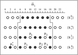
Figure 3: System with $N=12$ sites. Fermion momenta $k_{i}=(\pi/N)\bar{m}_{i}$ for the lowest energy states at $N_{f}=N/2$ (row 1) and $N_{f}=N/2-1$ (row 2). Also shown are the fermion momenta for a generic 2-spinon state (row 3) and a generic 4-spinon state in the subspace with $N_{f}=N/2-1$. Also shown are segments of the two-pronged fork described in the context of Fig. 2

In $S_{zz}(q,\omega)_{0}$ the only non-vanishing transition rates (3.8) pertain to the set of 2-spinon excitations (with $n_{+}=n_{-}=1$). In the fermion representation they are 1-particle-1-hole states relative to the ground state, generated from row 1 of Fig. 3 by moving exactly one fermion from the inside domain to the outside domain. The total number of such states is $N^{2}/4$, each contributing the amount $1/N$ to the spectral weight. Parenthetically, let us mention the polymer fluctuation operator $P_{q}^{2M},M=1,2,3,\ldots$ introduced in Ref. [20]. This operator only allows transitions from the spinon vacuum to the set of $2M$-spinon excitations (with $n_{+}=n_{-}=M$), i.e. to the set of $M$-particle-$M$-hole excitations in the fermion representation.

Our main focus here is on $S_{-+}(q,\omega)_{0}$. Note that we have $S_{-+}(q,\omega)_{0}=S_{+-}(q,\omega)_{0}$ due to reflection symmetry in spin space, even though the two functions involve different sets of excited states. All excitations in the invariant subspace with $N_{f}=N/2-1$ contribute spectral weight to $S_{-+}(q,\omega)_{0}$. For their systematic generation it is useful to start from the state with the lowest energy in that subspace. It has spinon composition $n_{+}=2,n_{-}=0$ and its fermion momenta $\{k_{i}^{-}\}$ are illustrated in row 2 of Fig. 3.

The complete set of 2-spinon states in the same invariant subspace can now be described by two even-valued integer parameters $N/2\leq\mu_{1}<\mu_{2}\leq 3N/2$ as illustrated in row 3 of Fig. 3. They mark the two vacancies in the array of fermion momenta $\{k_{i}^{2}\}$ in the inside domain. These vacancies represent spinons with spin up $(n_{+}=2)$. The spinon momenta are determined by the rules given in Sec. 2.

The 4-spinon excitations relevant for $S_{-+}(q,\omega)_{0}$ have $n_{+}=3$ and $n_{-}=1$. The spin-up spinons are described by three even-valued integer parameters $N/2\leq\mu_{1}<\mu_{2}<\mu_{3}\leq 3N/2$ as shown in row 4 of Fig. 3. The spin-down spinon is described by the even-valued integer parameter $\mu_{1}^{*}$ in the outside domain i.e. with range $0\leq\mu_{1}^{*}<N/2$ or $3N/2<\mu_{1}^{*}<2N$. In generalization to this recipe, the $m$-spinon excitations contributing to $S_{-+}(q,\omega)_{0}$ have $n_{+}=m/2+1,n_{-}=m/2-1$, generated by moving $m/2-1$ fermions from the inside domain to the outside domain (with parameters $\mu_{1}^{*},\ldots,\mu_{m/2-1}^{*}$) and thus leaving $m/2+1$ vacancies inside (with parameters $\mu_{1},\ldots,\mu_{m/2+1}$).

3.3 Total $m$-spinon intensity for even $N$

How is the total spectral intensity in the dynamic spin structure factor $S_{-+}(q,\omega)$ divided among the $m$-spinon excitations? From a previous study based on algebraic analysis [21] we know that in the axial regime of the $XXZ$ antiferromagnet most of the spectral weight is carried by the 2-spinon excitations alone. On the other hand, previous Bethe ansatz studies [17, 15] yielded evidence that in the planar regime the 2-spinon contribution approaches zero in the limit $N\to\infty$.

By using the transition rate expressions (3.7) we have produced numerical data for the relative 2-spinon intensity $I_{2}/I_{\rm tot}$ and the relative 4-spinon intensity $I_{4}/I_{\rm tot}$, where

$$I_{\rm tot}=\sum_{q}\sum_{n}M^{-}_{0n}(q)=\sum_{m=2,4,\ldots}I_{m}=\frac{N}{2}.$$ (3.12)

The data are shown in Fig. 4. We see that the 2-spinon intensity accounts for more than half the total intensity in chains with up to at least $N\simeq 300$ sites. Nevertheless, the data are consistent with the conclusion that the relative 2-spinon intensity drops to zero in the limit $N\to\infty$.

Figure 4: Relative overall intensity of the 2-spinon excitations ($\circ$) and 4-spinon excitations ($\bullet$) in $S_{-+}(q,\omega)_{0}$ plotted versus $1/N$.

The relative contribution of the 4-spinon excitations first rises with $N$. It levels off at $\sim 48\%$ for $N\simeq 2000$ and then starts to decrease. In all likelihood, the relative 4-spinon intensity and, for that matter, any relative $m$-spinon intensity taken individually, will vanish in the limit $N\to\infty$. However, the combined 2-spinon and 4-spinon relative intensity stays above 80% for chains with up to $N\simeq 2000$ sites.

3.4 Asymptotic transition rates for even $N$

How is the $m$-spinon intensity of $S_{-+}(q,\omega)_{0}$ distributed in the $(q,\omega)$-plane for large $N$? To answer this question we must determine the explicit dependence of the transition rate expression (3.7) on the spectral parameters $q$ and $\omega$. The product nature of (3.7) suggests the following factorization of the transition rate expression between the spinon vacuum and an $m$-spinon state (for $m=2,4,\ldots$):

$$M^{-}\big{(}\{k_{i}^{0}\},\{k_{i}^{m}\}\big{)}=\underset{\mathrm{scaled\;transition\;rate}}{\underbrace{\frac{M^{-}\big{(}\{k_{i}^{0}\},\{k_{i}^{m}\}\big{)}}{M^{-}\big{(}\{k_{i}^{0}\},\{k_{i}^{-}\}\big{)}}}}\times\underset{\mathrm{scaling\;factor}}{\underbrace{\rule[-11.38109pt]{0.0pt}{25.60747pt}M^{-}\big{(}\{k_{i}^{0}\},\{k_{i}^{-}\}\big{)}.}}$$ (3.13)

Here $\{k_{i}^{0}\}$ and $\{k_{i}^{-}\}$ are the fermion momenta of the lowest state in the invariant Hilbert subspaces with $N/2$ fermions and $N/2-1$ fermions, respectively. The fermion momenta $\{k_{i}^{m}\}$ of an arbitrary $m$-spinon excitation differ from the set $\{k_{i}^{-}\}$ as explained in the context of Fig. 3. In the representation (3.13) we use the transition rate between the two reference states (second factor) as a common scaling factor for all $m$-spinon excitations. In the scaled transition rates (first factor), huge cancellations take place because different $m$-spinon excitations differ by no more than $m$ fermion momenta.

The asymptotic scaling factor must be calculated by expansions of the product expression

$$M^{-}\big{(}\big{\{}k_{i}^{0}\big{\}},\big{\{}k_{i}^{-}\big{\}}\big{)}=\sqrt{N}C_{N}(N/2),$$ (3.14)

$$C_{N}(n)\doteq\prod\limits_{l=1}^{n}\frac{\sin^{4l-3}\eta(l-1/2)}{\sin^{4l-1}\eta l},\qquad\eta\doteq\frac{\pi}{N}$$ (3.15)

as inferred from (3.7) for the two specific states. The result is of the form

$$M^{-}\big{(}\big{\{}k_{i}^{0}\big{\}},\big{\{}k_{i}^{-}\big{\}}\big{)}\stackrel{{\scriptstyle a}}{{=}}\sqrt{N}C,$$ (3.16)

where here and henceforth the symbol “$\stackrel{{\scriptstyle a}}{{=}}$” denotes an asymptotic equality for large $N$ that ignores corrections of the kind $\times[1+\mathcal{O}(N^{-1})]$. The constant

$$C \doteq \lim_{N\to\infty}C_{N}(N/2)$$

$$= \sqrt{\pi}\exp\left(\frac{\ln 2}{6}+6\zeta^{\prime}(-1)\right)=0.73739071\ldots,$$

where $\zeta(z)$ is the Riemann zeta function is familiar from previous calculations of correlation functions for the $XX$ model by a different approach [5]. We now present explicit results for the 2-spinon and 4-spinon transition rates.

3.5 Asymptotic $2$-spinon transition rates

The scaled transition rate for a 2-spinon excitation can be reduced to the following product:

$$\frac{M^{-}\big{(}\{k_{i}^{0}\},\{k_{i}^{2}\}\big{)}}{M^{-}\big{(}\{k_{i}^{0}\},\{k_{i}^{-}\}\big{)}}=N^{2}\sin^{2}\frac{\kappa_{1}-\kappa_{2}}{2}\prod_{j=1}^{2}\phi(\psi_{j})\phi(N/2-\psi_{j})$$ (3.18)

with the function

$$\phi(n)\doteq\prod_{l=1}^{n}\frac{\sin^{2}\eta(l-\frac{1}{2})}{\sin^{2}\eta l},\qquad n\in\mathbb{N}^{+},\qquad\phi(0)\doteq 1,$$ (3.19)

depending on two parameters $\mu_{1}$ and $\mu_{2}$ via

$$\psi_{i}=\frac{\mu_{i}}{2}-\frac{N}{4},\quad\kappa_{i}=\eta\mu_{i},\qquad i=1,2.$$ (3.20)

Performing the limit $N\to\infty$ is delicate because of singularities along the spectral boundaries of the 2-spinon excitations. To leading order in $N$, expression (3.18) becomes

$$\frac{M^{-}\big{(}\{k_{i}^{0}\},\{k_{i}^{2}\}\big{)}}{M^{-}\big{(}\{k_{i}^{0}\},\{k_{i}^{-}\}\big{)}}\stackrel{{\scriptstyle a}}{{=}}\frac{4}{N^{2}}\frac{\displaystyle\sin^{2}\frac{\kappa_{1}-\kappa_{2}}{2}}{\cos\kappa_{1}\cos\kappa_{2}},$$ (3.21)

where the two parameters $\kappa_{1},\kappa_{2}$ are related to the energy transfer $\omega$ and momentum transfer $q$ as follows:

$$\omega\stackrel{{\scriptstyle a}}{{=}}-\sum_{i=1}^{2}\cos\kappa_{i},\qquad q=\pi-\sum_{i=1}^{2}\kappa_{i}~{}\mathrm{mod}~{}2\pi.$$ (3.22)

Note that the limits $\{k_{i}^{2}\}\to\{k_{i}^{-}\}$ and $N\to\infty$ are not interchangeable. Hence we cannot recover the unit value of the scaled transition rate by taking the limit $\kappa_{1}-\kappa_{2}\to\pi$ and $\kappa_{1}+\kappa_{2}\to 2\pi$ in the asymptotic expression (3.21).

Assembling the results (3.16) and (3.21) with (3.22) into (3.13) yields the 2-spinon transition rate function

$$M_{2}^{-}(q,\omega)\stackrel{{\scriptstyle a}}{{=}}\frac{4C}{N^{3/2}}\,\frac{4\sin^{2}(q/2)-\omega^{2}}{\omega^{2}-\sin^{2}q}$$ (3.23)

over the (asymptotic) range $|\sin q|\leq\omega\leq 2|\sin(q/2)|$ of the 2-spinon spectrum. The 2-spinon part of the dynamic spin structure factor $S_{-+}(q,\omega)_{0}$ is then obtained by multiplying the 2-spinon transition rate function (3.23) with the 2-spinon density of states,

$$D_{2}(q,\omega)\stackrel{{\scriptstyle a}}{{=}}\frac{N}{2\pi}\frac{1}{\sqrt{4\sin^{2}(q/2)-\omega^{2}}},$$ (3.24)

yielding

$$S_{-+}^{(2)}(q,\omega)_{0}\stackrel{{\scriptstyle a}}{{=}}\frac{2C}{\pi\sqrt{N}}\frac{\sqrt{4\sin^{2}(q/2)-\omega^{2}}}{\omega^{2}-\sin^{2}q}.$$ (3.25)

The interpretation of the asymptotic result (3.25) requires caution. It is indicative of the 2-spinon spectral-weight distribution in the following sense: in a histogram plot of $S_{-+}^{(2)}(q,\omega)_{0}$ based on the transition rates (3.7), the shape of (3.25) comes into better and better focus as $N$ grows larger, while the relative intensity of this structure fades away.

3.6 Asymptotic $4$-spinon transition rates

We start again from the factorized expression (3.13). The asymptotic scaling factor remains the same: Eq. (3.16). The surviving factors in the scaled transition rate after the massive cancellations now depend on four parameters (see Fig. 3):

$$\frac{M^{-}\big{(}\{k_{i}^{0}\},\{k_{i}^{4}\}\big{)}}{M^{-}\big{(}\{k_{i}^{0}\},\{k_{i}^{-}\}\big{)}} = N^{2}\sin^{2}\left(\frac{\kappa_{1}^{*}}{2}-\frac{\pi}{4}\right)\frac{\displaystyle\prod_{i<j}^{3}\sin^{2}\frac{\kappa_{i}-\kappa_{j}}{2}}{\displaystyle\prod_{i=1}^{3}\sin^{2}\frac{\kappa_{1}^{*}-\kappa_{i}}{2}}$$ (3.26)

$$\times\frac{\phi(N/4-\mu_{1}^{*}/2)}{\phi(3N/4-\mu_{1}^{*}/2)}\prod_{j=1}^{3}\phi(\psi_{j})\phi(N/2-\psi_{j})$$

where

$$\psi_{i}=\frac{\mu_{i}}{2}-\frac{N}{4},\quad\kappa_{i}=\eta\mu_{i},\quad i=1,2,3,\qquad\kappa_{1}^{*}=\eta\mu_{1}^{*}.$$ (3.27)

From this result we have derived the following asymptotic expression for the scaled 4-spinon transition rates:

$$\frac{M^{-}\big{(}\{k_{i}^{0}\},\{k_{i}^{4}\}\big{)}}{M^{-}\big{(}\{k_{i}^{0}\},\{k_{i}^{-}\}\big{)}} \stackrel{{\scriptstyle a}}{{=}} \frac{4}{N^{4}}\,\frac{\cos(\kappa_{1}^{*})}{\displaystyle\prod_{i=1}^{3}\cos(\kappa_{i})}\frac{\displaystyle\prod_{i<j}^{3}\sin^{2}\frac{\kappa_{i}-\kappa_{j}}{2}}{\displaystyle\prod_{i=1}^{3}\sin^{2}\frac{\kappa_{1}^{*}-\kappa_{i}}{2}}$$ (3.28)

The asymptotic dependence of the energy and momentum transfer of 4-spinon excitations on the four parameters is

$$\omega\stackrel{{\scriptstyle a}}{{=}}\cos\kappa_{1}^{*}-\sum_{i=1}^{3}\cos\kappa_{i},\qquad q=\pi+\kappa_{1}^{*}-\sum_{i=1}^{3}\kappa_{i}~{}\mathrm{mod}~{}2\pi.$$ (3.29)

From inspection of the 2-spinon result (3.21) and the 4-spinon result (3.28) we can already see features of the general structure for the $m$-spinon result emerging.

Figure 5: Excitation energy versus wave number of all 2-spinon $(\circ)$ and 4-spinon $(\cdot)$ excitations for $N=64$. The solid lines are the spectral boundaries for $N\to\infty$.

The range of the 4-spinon excitations in the $(q,\omega)$-plane in relation to the range of the 2-spinon excitations is illustrated in Fig. 5 for $N=64$ and asymptotically for $N\to\infty$. We can discern the nonuniform density of 2-spinon states (3.24) in the distribution of circles. Furthermore, from the distribution of dots we see that the density of 4-spinon excitations is very small near the spectral threshold and remains relatively small at energies $\omega\lesssim 1$. In the limit $N\to\infty$, the 2-spinon and 4-spinon excitations have a common spectral threshold,

$$\epsilon_{2L}(q)=\epsilon_{4L}(q)=|\sin q|,$$ (3.30)

and different upper boundaries,

$$\epsilon_{2U}(q)=2\left|\sin\,\frac{q}{2}\right|,$$ (3.31)

$$\epsilon_{4U}(q)=4\,\mathrm{max}\left[\;\left|\sin\,\frac{q}{4}\right|,\left|\sin\,\frac{q-2\pi}{4}\right|\;\right].$$ (3.32)

3.7 Transitions from the ground state for odd $N$

For odd $N$ the ground state is fourfold degenerate. Two of its vectors (labeled $A$ and $A^{\prime}$) are located in the invariant subspace with $N_{f}=(N-1)/2$ fermions and the other two vectors (labeled $B$ and $B^{\prime}$) in the subspace with $N_{f}=(N+1)/2$ fermions. We then have to consider transitions from each of the four ground-state vectors to the sets of $m$-spinon excitations with $m=1,3,\ldots$ in the accessible invariant subspaces. Without loss of generality we assume that $(N+1)/4$ is an integer.

The fermion momentum configurations of two of the four ground states are shown in rows 1 and 4 of Fig. 6 for $N=11$. It will suffice to consider these two vectors (with fermion momenta $\{k_{1}^{0},\ldots,k_{N/2-1}^{0}\}_{A}$ and $\{k_{1}^{0},\ldots,k_{N/2+1}^{0}\}_{B}$) and calculate from them the functions $S_{\mu\nu}(q,\omega)_{A}$ and $S_{\mu\nu}(q,\omega)_{B}$. Symmetry dictates that the other two ground state vectors yield the functions $S_{\mu\nu}(q,\omega)_{A^{\prime}}=S_{\mu\nu}(-q,\omega)_{A}$ and $S_{\mu\nu}(q,\omega)_{B^{\prime}}=S_{\mu\nu}(-q,\omega)_{B}$. Hence the $T=0$ dynamic spin structure factor (3.1) for odd $N$ can be rewritten as

$$S_{\mu\nu}(q,\omega)=\frac{1}{4}\left[S_{\mu\nu}(q,\omega)_{A}+S_{\mu\nu}(-q,\omega)_{A}+S_{\mu\nu}(q,\omega)_{B}+S_{\mu\nu}(-q,\omega)_{B}\right].$$ (3.33)

Different sets of excitations are again relevant for $\mu\nu=zz,+-,-+$.

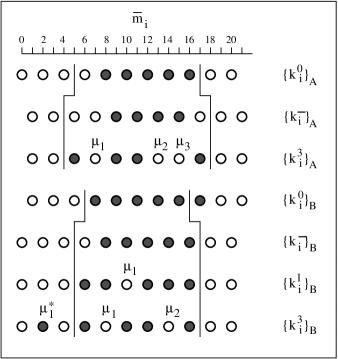
Figure 6: $XX$ chain with $N=11$ sites. Fermion momenta $k_{i}=(\pi/N)\bar{m}_{i}$ for one of two lowest energy states at $N_{f}=(N-1)/2$ (rows 1 and 5), $N_{f}=(N-3)/2$ (row 2), and $N_{f}=(N+1)/2$ (row 4). The other state in each case (henceforth referred to by subscripts $A^{\prime}$ or $B^{\prime}$) is obtained via reflection at the line $\bar{m}_{i}=11$. Also shown are the fermion momenta for a generic 1-spinon state in the subspace with $N_{f}=(N-1)/2$ (row 6), a generic 3-spinon state in the subspace with $N_{f}=(N-3)/2$ (row 3), and a generic 3-spinon state in the subspace with $N_{f}=(N-1)/2$ (row 7).

In $S_{zz}(q,\omega)_{A}$ the non-vanishing transition rates (3.8) now include all $(N+1)/2$ 1-spinon states (with $n_{+}=1$), including the ground-state vector $A$ itself, and a subset of $(N-1)^{2}/4$ 3-spinon states (with $n_{+}=2,n_{-}=1$), all in the same invariant subspace. In row 1 of Fig. 6 the 1-spinon states are obtained by moving the vacancy to any site in the inside domain, whereas the contributing 3-spinon excitations are obtained by leaving the vacancy inside as is and moving one particle from anywhere inside to anywhere outside. The relevant spectrum of $S_{zz}(q,\omega)_{B}$ is identified in like manner by starting from row 4 and interchanging the roles of the two domains and the roles of particles and vacancies.

As in Sec. 3.2 our main focus is on $\mu\nu=-+$. The spectrum for $S_{-+}(q,\omega)_{A}$ includes all eigenstates with $N_{f}=(N-3)/2$ and the spectrum for $S_{-+}(q,\omega)_{B}$ all eigenstates with $N_{f}=(N-1)/2$. For a systematic generation of all relevant excitations we again consider one state each in the invariant subspaces with $N_{f}=(N-3)/2$ and $N_{f}=(N-1)/2$ as reference states for the scaled matrix elements. These two states have fermion momentum configurations $\{k_{1}^{-},\ldots,k_{(N-3)/2}^{-}\}_{A}$ and $\{k_{1}^{-},\ldots,k_{(N-1)/2}^{-}\}_{B}$ as illustrated (for $N=11$) in rows 2 and 5, respectively, of Fig. 6.

Reference state $\{k_{i}^{-}\}_{A}$ is a 3-spinon state (with $n_{+}=2,n_{-}=1$) whereas reference state $\{k_{i}^{-}\}_{B}$ is a 1-spinon state (with $n_{+}=1$). The remaining states in the subspace of $\{k_{i}^{-}\}_{A}$ are $m$-spinon states for $m=3,5,\ldots$ with $n_{+}=(m+3)/2,n_{-}=(m-3)/2$, whereas the remaining states in the subspace of $\{k_{i}^{-}\}_{B}$ are $m$-spinon states for $m=1,3,\ldots$ with $n_{+}=(m+1)/2,n_{-}=(m-1)/2$. The 1-spinon and 3-spinon states thus generated are illustrated for $N=11$ in rows 3, 6, and 7 of Fig. 6. Note in particular that 1-spinon excitations only occur in $S_{-+}(q,\omega)_{B}$ but not in $S_{-+}(q,\omega)_{A}$.

We have produced extensive finite-$N$ data for the relative 1-spinon intensity $I_{1}^{B}/I_{\rm tot}^{B}$ and the relative 3-spinon intensities $I_{3}^{A}/I_{\rm tot}^{A}$ and $I_{3}^{B}/I_{\rm tot}^{B}$, where

$$I_{\rm tot}^{A} = \sum_{q}\sum_{n}M^{-}_{An}(q)=\sum_{m=3,5,\ldots}I_{m}^{A}=\frac{N-1}{2},$$

$$I_{\rm tot}^{B} = \sum_{q}\sum_{n}M^{-}_{Bn}(q)=\sum_{m=1,3,\ldots}I_{m}^{B}=\frac{N+1}{2}.$$ (3.34)

Figure 7: Relative overall intensity of the 1-spinon excitations $(\blacksquare$) and 3-spinon excitations $(\circ)$ in $S_{-+}(q,\omega)_{B}$ , and of the 3-spinon excitations $(\bullet$) in $S_{-+}(q,\omega)_{A}$, all plotted versus $1/N$.

The data are shown in Fig. 7. We see that the contribution of the 1-spinon excitations to the total intensity remains significant for chains with up to several hundred sites and the contribution of 3-spinon excitations for chains up to several thousand sites. Nevertheless, the data give a clear indication that both contributions vanish in the limit $N\to\infty$.

3.8 Asymptotic transition rates for odd $N$

In the factorization (3.13) we now have to distinguish two scaling factors for the degenerate ground state. Both must be calculated anew, from the product expressions

$$M^{-}\big{(}\{k_{i}^{0}\}_{A},\{k_{i}^{-}\}_{A}\big{)}=\sqrt{N}C_{N}((N-1)/2)\cos^{2}\frac{\eta}{2},$$ (3.35)

$$M^{-}\big{(}\{k_{i}^{0}\}_{B},\{k_{i}^{-}\}_{B}\big{)}=\sqrt{N}C_{N}((N-1)/2),$$ (3.36)

with $C_{N}((N-1)/2)$ defined in (3.15). The asymptotic results are again of the form

$$M^{-}\big{(}\{k_{i}^{0}\}_{A},\{k_{i}^{-}\}_{A}\big{)}\stackrel{{\scriptstyle a}}{{=}}M^{-}\big{(}\{k_{i}^{0}\}_{B},\{k_{i}^{-}\}_{B}\big{)}\stackrel{{\scriptstyle a}}{{=}}\sqrt{N}C$$ (3.37)

with the constant $C$ from (3.4).

The scaled transition rate for a 1-spinon excitation is reduced to

$$\frac{M^{-}\big{(}\{k_{i}^{0}\}_{B},\{k_{i}^{1}\}_{B}\big{)}}{M^{-}\big{(}\{k_{i}^{0}\}_{B},\{k_{i}^{-}\}_{B}\big{)}}=N\cos^{2}(\eta\psi_{1})\phi(\psi_{1})\phi((N-1)/2-\psi_{1}),$$ (3.38)

where

$$\psi_{1}=\frac{\mu_{1}}{2}-\frac{N+1}{4},\quad\kappa_{1}=\eta\mu_{1}.$$ (3.39)

Asymptotically for $N\to\infty$ Eq. (3.38) becomes

$$\frac{M^{-}\big{(}\{k_{i}^{0}\}_{B},\{k_{i}^{1}\}_{B}\big{)}}{M^{-}\big{(}\{k_{i}^{0}\}_{B},\{k_{i}^{-}\}_{B}\big{)}}\stackrel{{\scriptstyle a}}{{=}}\frac{1}{N}\cot\left(\frac{\kappa_{1}}{2}-\frac{\pi}{4}\right).$$ (3.40)

The 1-spinon energy and momentum transfers are

$$\omega\stackrel{{\scriptstyle a}}{{=}}-\cos\kappa_{1},\qquad q\stackrel{{\scriptstyle a}}{{=}}\frac{3\pi}{2}-\kappa_{1}.$$ (3.41)

Note again that the limits $\{k_{i}^{1}\}_{B}\to\{k_{i}^{-}\}_{B}$ and $N\to\infty$ are no longer interchangeable in the asymptotic result. The 1-spinon transition rate function thus becomes

$$M_{1}^{-}(q,\omega)_{B}\stackrel{{\scriptstyle a}}{{=}}\frac{C}{\sqrt{N}}\tan\frac{q}{2}.$$ (3.42)

Taking into account the fourfold ground-state degeneracy, we can write the asymptotic expression for the 1-spinon part of the dynamic spin structure factor in the form

$$S_{-+}^{(1)}(q,\omega)\stackrel{{\scriptstyle a}}{{=}}\frac{C}{4\sqrt{N}}\tan\frac{q}{2}\delta\left(\omega-|\sin q|\right).$$ (3.43)

Different sets of 3-spinon states are reached via $S_{q}^{-}$ from the ground-state components $A$ and $B$. Hence we must work with two different results for the scaled transition rates. For ground-state $B$ we obtain the expression

$$\frac{M^{-}\big{(}\{k_{i}^{0}\}_{B},\{k_{i}^{3}\}_{B}\big{)}}{M^{-}\big{(}\{k_{i}^{0}\}_{B},\{k_{i}^{-}\}_{B}\big{)}}=N\tan^{2}(\eta\psi_{1}^{*})\sin^{2}(\eta(\psi_{1}-\psi_{2}))\prod_{j=1}^{2}\frac{\cos^{2}(\eta\psi_{j})}{\sin^{2}(\eta(\psi_{1}^{*}-\psi_{j}))}$$

$$\times\frac{\phi(-\psi_{1}^{*})}{\phi((N-1)/2-\psi_{1}^{*})}\prod_{j=1}^{2}\phi(\psi_{j})\phi((N-1)/2-\psi_{j})$$ (3.44)

depending on the three parameters

$$\psi_{1}=\frac{\mu_{1}}{2}-\frac{N+1}{4},\quad\psi_{2}=\frac{\mu_{2}}{2}-\frac{N+1}{4},\quad\psi_{1}^{*}=\frac{\mu_{1}^{*}}{2}-\frac{N+1}{4}.\quad$$ (3.45)

The asymptotic expansion of (3.8) yields the following leading term, now parameterized by $\kappa_{1}=\eta\mu_{1}$, $\kappa_{2}=\eta\mu_{2}$, and $\kappa_{1}^{*}=\eta\mu_{1}^{*}$:

$$\frac{M^{-}\big{(}\{k_{i}^{0}\}_{B},\{k_{i}^{3}\}_{B}\big{)}}{M^{-}\big{(}\{k_{i}^{0}\}_{B},\{k_{i}^{-}\}_{B}\big{)}} \stackrel{{\scriptstyle a}}{{=}} \frac{1}{N^{3}}\,\frac{\displaystyle\sin^{2}\big{(}\frac{\kappa_{1}-\kappa_{2}}{2}\big{)}}{\displaystyle\prod_{i=1}^{2}\tan\big{(}\frac{\kappa_{i}}{2}-\frac{\pi}{4}\big{)}}\frac{\displaystyle\tan\big{(}\frac{\pi}{4}-\frac{\kappa^{*}_{1}}{2}\big{)}}{\displaystyle\prod_{i=1}^{2}\sin^{2}\big{(}\frac{\kappa^{*}_{1}-\kappa_{i}}{2}\big{)}}.$$ (3.46)

The energy transfer and momentum transfer in the asymptotic regime are

$$\omega\stackrel{{\scriptstyle a}}{{=}}\cos\kappa^{*}_{1}-\sum_{i=1}^{2}\cos\kappa_{i},\qquad q\stackrel{{\scriptstyle a}}{{=}}{\kappa^{*}_{1}-\sum_{i=1}^{2}\kappa_{i}-\frac{\pi}{2}}\quad\mathrm{mod}~{}2\pi.$$ (3.47)

Figure 8: Excitation energy versus wave number of all 1-spinon excitations ($\circ$) and 3-spinon excitations ($\cdot$) from ground-state $B$ for $N=63$. The solid lines are the 3-spinon continuum boundaries for $N\to\infty$. The corresponding 1-spinon and 3-spinon spectrum from ground-state $B^{\prime}$ is the mirror image reflected at $q/\pi=1$ of the spectrum shown.

The range in the $(q,\omega)$-plane of the 1-spinon and 3-spinon excitations from ground-state $B$ is shown in Fig. 8 for $N=63$. The corresponding spectrum reached from ground-state $B^{\prime}$ is the one with wave numbers $q$ replaced by $2\pi-q$. In the limit $N\to\infty$ the single branch of 1-spinon excitations coincides with the lower boundary of the 3-spinon continuum,

$$\epsilon_{1}(q)=\epsilon_{3L}(q)=|\sin\,q|.$$ (3.48)

The upper boundary of the 3-spinon continuum is

$$\epsilon_{3U}(q)=3\,\mathrm{max}\left[\;\left|\sin\,\frac{q}{3}\right|,\left|\sin\,\frac{q-2\pi}{3}\right|\;\right].$$ (3.49)

The scaled transition for 3-spinon transitions from ground-state $A$ reads

$$\frac{M^{-}\big{(}\{k_{i}^{3}\}_{A},\{k_{i}^{0}\}_{A}\big{)}}{M^{-}\big{(}\{k_{i}^{-}\}_{A},\{k_{i}^{0}\}_{A}\big{)}} = N^{3}\sin^{2}\frac{\eta}{2}\,\frac{\displaystyle\prod_{i<j}^{3}\sin^{2}(\eta(\psi_{i}-\psi_{j}))}{\displaystyle\prod_{j=1}^{3}\sin^{2}(\eta(\psi_{j}-1/2))}$$ (3.50)

$$\times \prod_{j=1}^{3}\phi(\psi_{j})\phi((N+1)/2-\psi_{j})$$

depending on the three parameters

$$\psi_{i}=\frac{\mu_{i}}{2}-\frac{N-1}{4},\quad i=1,2,3.$$ (3.51)

The leading term of the asymptotic expansion becomes a function of the three variables $\kappa_{i}=\eta\mu_{i}$:

$$\frac{M^{-}\big{(}\{k_{i}^{3}\}_{A},\{k_{i}^{0}\}_{A}\big{)}}{M^{-}\big{(}\{k_{i}^{-}\}_{A},\{k_{i}^{0}\}_{A}\big{)}}\stackrel{{\scriptstyle a}}{{=}}\frac{\pi^{2}}{4N^{5}}\frac{\displaystyle\prod_{i<j}^{3}\sin^{2}\frac{\kappa_{i}-\kappa_{j}}{2}}{\displaystyle\prod_{i=1}^{3}\cos\left(\frac{\kappa_{i}}{2}-\frac{\pi}{4}\right)\sin^{3}\left(\frac{\kappa_{i}}{2}-\frac{\pi}{4}\right)}$$ (3.52)

with associated energy and momentum transfer

$$\omega\stackrel{{\scriptstyle a}}{{=}}-\sum_{i=1}^{3}\cos\kappa_{i},\qquad q\stackrel{{\scriptstyle a}}{{=}}\frac{3\pi}{2}-\sum_{i=1}^{3}\kappa_{i}\quad\mathrm{mod}~{}2\pi.$$ (3.53)

Figure 9: Excitation energy versus wave number of all 3-spinon excitations ($\cdot$) from ground-state $A$ for $N=63$. The solid lines are the 3-spinon continuum boundaries for $N\to\infty$. The corresponding 3-spinon spectrum from the ground-state component $A^{\prime}$ is the mirror image reflected at $q/\pi=1$ of of the spectrum shown.

The range in the $(q,\omega)$-plane of the 3-spinon excitations from ground-state $A$ is shown in Fig. 9 for $N=63$. The corresponding spectrum reached from ground-state component $A^{\prime}$ is the one with wave numbers $q$ replaced by $2\pi-q$. In the limit $N\to\infty$ the 3-spinon continuum boundaries for states $A$ and $A^{\prime}$ combined are the same as those of states $B$ and $B^{\prime}$ combined.

4 Conclusion and outlook

The two main results on the $XX$ model reported in this paper are (i) the exact one-to-one mapping between fermion and spinon compositions of all eigenstates and (ii) the applications of exact product expressions for the transition rates as needed for the calculation of dynamic spin structure factors. The mapping has provided us with a framework that allows us to explore any property of interest by using the computationally convenient (free) fermion quasiparticles and interpret the results in terms of the physically relevant (interacting) spinon quasiparticles. The very product nature of the transition rate expressions for the $XX$ model has put us at a huge advantage in the face of the equivalent determinantal expressions known for the $XXZ$ model in general, when it comes to the evaluation of explicit numerical results or the calculation of asymptotic analytic results for large systems.

The applications worked out in Sec. 3 call for a new assessment of some issues and set the stage for the pursuit of new questions of interest. Chief among the issues that need to be reevaluated in the light of the results reported here concerns the role in general and the observability in particular of specific sets of spinon quasiparticles in dynamic spin structure factors and related quantities.

The evidence presented in Sec. 3 suggests that the relative intensity of any individual $m$-spinon contribution to the dynamic spin structure factor $S_{-+}(q,\omega)$ at $T=0$ vanishes in the limit $N\to\infty$. This conclusion, which is expected to hold true not only for the $XX$ model but within the entire planar regime of the $XXZ$ model [17], is in contrast to what is known on rigorous grounds for the $XXZ$ model in the axial regime including the isotropic limit ($XXX$ model): the relative intensity of the 2-spinon excitations alone amounts to 73% in the Heisenberg limit and gradually increases to 100% in the Ising limit [22, 21].

The dominant singularities in the dynamic structure factor have been shown to be extractable from the 2-spinon part alone in the $XXX$ model [22]. This is manifestly not the case in the $XX$ model and unlikely the case for the planar $XXZ$ model in general. A fair amount of exact information about the singularity structure of $S_{-+}(q,\omega)$ at $T=0$ can be gleaned from existing results [5, 8, 9, 10, 11]. One important task will be to assemble the asymptotic $m$-spinon results from the approach taken here to recover known exact results for $N\to\infty$. A hopeful sign for this endeavor is that the constant $C$ as given in (3.4), which plays a crucial role in exact results for $N\to\infty$, already emerges from the asymptotic $m$-spinon expressions worked out here.

Dynamic spin structure factors are accessible more or less directly to experimental investigations via neutron scattering, NMR, ESR, light scattering, and other probes in the context of quasi-one-dimensional magnetic compounds. Even small amounts of impurities or other defects will turn a crystalline sample into an ensembles of mesoscopic chains of various lengths $(N\sim 10^{2}-10^{3})$. Under what circumstances does the distinction between a physical ensemble of mesoscopic chains and a statistical ensemble of macroscopic chains matter?

If the relative intensity of the 2-spinon contribution is dominant for mesoscopic chains as well as for macroscopic chains, which is the case for the $XXX$ model and the axial $XXZ$ model, then the distinction has minimal impact. If, on the other hand, the relative 2-spinon intensity is dominant for chains of length $N\sim 10^{2}$ and the relative 4-spinon intensity is dominant for chains of length $N\sim 10^{3}$ but both contributions taken individually or combined become negligible in macroscopic chains, as is the case in the $XX$ model, then the distinction cannot be ignored. Hence the significance of the results presented in Sec. 3.

In conclusion we mention two further unresolved issues to which the work reported here has led. They are the subject of work currently in progress. A first set of questions calls for a derivation of the product expressions (3.6)-(3.7) and for the establishment of connections to the many exact results for dynamic correlation functions already known for the $XX$ model. A second set of questions calls for a detailed study of the spinon interaction and for the exploration of the physical relevant quasiparticles whose physical vacuum is the $XX$ ground state in a magnetic field.

References

References

- [1] Lieb E, Schulz T and Mattis D, 1961 Ann. Phys. 16 407
- [2] Katsura S, 1962 Phys. Rev. 127 1508
- [3] Niemeijer T, 1967 Physica 36 377
- [4] Katsura S, Horiguchi T and Suzuki M, 1970 Physica 46 67
- [5] McCoy B M, Barouch E and Abraham D B, 1971 Phys. Rev. A 4 2331
- [6] Brandt U and Jacoby K, 1976 Z. Phys. 25 181
- [7] Capel H W and Perk J H H, 1977 Physica A87 211
- [8] Vaidya H G and Tracy C A, 1978 Physica 92 A 1
- [9] Müller G and Shrock R E, 1984 Phys. Rev. B 29 288
- [10] McCoy B M, Perk J H H and Shrock R E, 1983 Nucl. Phys. B 220 35
- [11] McCoy B M, Perk J H H and Shrock R E, 1983 Nucl. Phys. B 220 269
- [12] Its A R, Izergin A G, Korepin V E and Slavnov N A, 1993 Phys. Rev. Lett. 70 1704
- [13] Stolze J, Nöppert A and Müller G, 1995 Phys. Rev. B 52 4319
- [14] Derzhko O, Krokhmalskii T and Stolze J, 2000 J. Phys. A: Math. Gen. 33 3063
- [15] Biegel D, Karbach M, Müller G and Wiele K, (2004) Phys. Rev. B 69 174404
- [16] Haldane F D M, 1991 Phys. Rev. Lett. 67 937
- [17] Biegel D, Karbach M and Müller G, 2003 J. Phys. A: Math. Gen. 36 5361
- [18] Kitanine N, Maillet J M and Terras V, 1999 Nucl. Phys. B 554 647
- [19] Korepin V E, Bogoliubov N M and Izergin A G, Quantum Inverse Scattering Method and Correlation Functions (Cambridge University Press, Cambridge, 1993)
- [20] Derzhko O, Krokhmalskii T, Stolze J and Müller G, 2005 Phys. Rev. B 71 104432
- [21] Bougourzi A H, Karbach M and Müller G, 1998 Phys. Rev. B 57 11429
- [22] Karbach M, Müller G, Bougourzi A H, Fledderjohann A et al., 1997 Phys. Rev. B 12510