The spin glass transition of the three dimensional Heisenberg spin glass.

Abstract

It is shown, by means of Monte Carlo simulation and Finite Size Scaling analysis, that the Heisenberg spin glass undergoes a finite-temperature phase transition in three dimensions. There is a single critical temperature, at which both a spin glass and a chiral glass orderings develop. The Monte Carlo algorithm, adapted from lattice gauge theory simulations, makes possible to thermalize lattices of size $L=32$, larger than in any previous spin glass simulation in three dimensions. High accuracy is reached thanks to the use of the Marenostrum supercomputer. The large range of system sizes studied allow us to consider scaling corrections.

Recently, decisive evidence for a spin glass transition SGINTRO in three dimensional Ising spin glasses was found by us BALLESTEROS and by Palassini and Caracciolo PALASS-CARACC . These works demonstrated the applicability to spin-glasses of our approach QUOTIENTS ; VICTORAMIT to Finite Size Scaling (FSS) at the critical temperature, as well as that of Caracciolo and coworkers FSS-PISA for the paramagnetic state (see also JORG ; KATZYOUNG ).

However, the situation is still confusing for Heisenberg spin glasses Tc0 ; MATSUBARA ; IMAGAWA ; VILLAIN ; QUIRALES ; QUIRALESNEW ; YOUNG ; OTROS ; FELIX , which is the more experimentally interesting case (see e.g. MEM-REJ-BERT ; HEISS-H-EXP ). Indeed, numerical studies are the only theoretical tool to achieve progress in three dimensions. Early simulations Tc0 could not reach low enough temperatures due to the dramatic dynamical arrest of the algorithms available at the time, and concluded that the critical temperature, $T_{\mathrm{c}}$, was strictly zero. Yet, recent studies at lower temperatures OTROS ; FELIX found indirect indications of a spin glass transition for Heisenberg spin glasses. Matters are further complicated by the Villain et al. VILLAIN suggestion of a low temperature chiral glass phase, with an Ising like ordering due to the handedness of the non-collinear spin structures (see definitions below). The simulations of Kawamura and coworkers QUIRALES ; QUIRALESNEW gave ample support to this spin-chirality decoupling scenario (i.e. $T_{\mathrm{c}}=0$ for the spin glass, but $T_{\mathrm{c}}>0$ for the chiral glass ordering).

In order to clarify the situation for Heisenberg and XY spin glasses in $D=3$, Young and Lee YOUNG have recently tried our FSS methods at $T_{\mathrm{c}}$ BALLESTEROS ; QUOTIENTS . Although parallel tempering only allowed them YOUNG to thermalize systems of size up to $L=12$, very clear results were reached for the XY spin glasses. The finite-lattice correlation length COOPER , $\xi_{L}$, was analyzed for several system sizes $L$. As expected QUOTIENTS ; BALLESTEROS ; VICTORAMIT , the dimensionless ratio $\xi_{L}/L$ crosses neatly at the same $T_{\mathrm{c}}$, for the chiral glass and the spin glass ordering, for XY spin glasses. In the more important case of Heisenberg spin glasses, their results, although inconclusive, were interpreted also as lack of spin-chirality decoupling. This conclusion has been criticized by Kawamura and Hukushima QUIRALESNEW , that studied somehow larger systems on very few samples.

Here we show that a finite-temperature spin glass transition occurs for the Heisenberg spin glass in $D=3$. The critical temperature for the spin glass transition coincides with that of the chiral glass. Our results rely on Monte Carlo simulation and FSS analysis at $T_{\mathrm{c}}$ QUOTIENTS ; BALLESTEROS ; VICTORAMIT . We adapt a lattice gauge theory algorithm OVERRELAX to our problem. Our algorithm thermalizes $L=32$ systems, well beyond any previous spin glass simulation in $D=3$. The use of Marenostrum, one of the World largest computing facilities, during (the equivalent of) $2.6\times 10^{4}$ Pentium IV computing days allowed us to simulate 4000 samples. The phase transition seems to be of Kosterlitz-Thouless type KOST-THOU , although we may not exclude a lower critical dimension barely smaller than three.

We consider the Edwards-Anderson model. The Heisenberg spins $\vec{S_{i}}=(S_{i}^{x},S_{i}^{y},S_{i}^{z})$, $\vec{S_{i}}\cdot\vec{S_{i}}=1\,$, live on the nodes a cubic lattice of size $L$, with periodic boundary conditions. Spins interact via the Hamiltonian ($\langle ij\rangle$ indicates sum over all pairs of lattice nearest neighbors):

$$H=-\sum_{\langle i,j\rangle}J_{ij}\vec{S_{i}}\cdot\vec{S_{j}}\,.$$ (1)

The $J_{ij}$ are Gaussian distributed quenched random couplings SGINTRO . Their mean value is zero, while their variance sets the energy unit. For any quantity, $O$, we first calculate the thermal average for the given couplings, $\langle O\rangle_{J}$. The average over the $J_{ij}$, $\overline{\langle O\rangle_{J}}$, is only taken afterward.

In order to detect non-planar spin structures, one forms the chiral (pseudovector) density field QUIRALES :

$$\zeta_{i\mu}=\vec{S}_{i+\hat{e}_{\mu}}\cdot(\vec{S}_{i}\times\vec{S}_{i-\hat{e}_{\mu}})\quad(\mu=x,y,z)\,,$$ (2)

where $\hat{e}_{\mu}$ is the unit lattice vector along the $\mu$ axis.

We introduce real replicas SGINTRO : pairs of spin configurations, $\vec{S}_{i}^{(1)}$ and $\vec{S}_{i}^{(2)}$ independently evolving with the same set of couplings, $\{J_{ij}\}$, and at the same temperature, $T$. We have as well a replicated field for the chiral densities, (2). From the real replicas we form the tensor field $q_{\mu\nu}(\vec{r}_{i})$ and the chiral vector field $\kappa_{i,\mu}$: ($\mu,\nu=x,y,z$)

$$q_{\mu,\nu}(\vec{r}_{i})=S_{i,\mu}^{(1)}S_{i,\nu}^{(2)}\,,\quad\kappa_{i,\mu}=\zeta_{i,\mu}^{(1)}\zeta_{i,\mu}^{(2)}\,.$$ (3)

Their Fourier transforms,

$$\hat{q}_{\mu,\nu}(\vec{k})=\sum_{i=1}^{N}\frac{q_{\mu,\nu}(\vec{r}_{i})\mathrm{e}^{\mathrm{i}\vec{k}\cdot\vec{r_{i}}}}{L^{3}}\,,\ \hat{\kappa}_{\mu}(\vec{k})=\sum_{i=1}^{N}\frac{\kappa_{i,\mu}\mathrm{e}^{\mathrm{i}\vec{k}\cdot\vec{r_{i}}}}{L^{3}}\,,$$ (4)

yield the spin glass (SG) wave vector dependent susceptibility and the chiral glass (CG) one:

$$\frac{\chi_{\mathrm{SG}}(\vec{k})}{L^{3}}=\sum_{\mu,\nu}\overline{\langle|\hat{q}_{\mu,\nu}(\vec{k})|^{2}\rangle_{J}}\,,\ \frac{\chi_{\mathrm{CG}}^{\mu}(\vec{k})}{L^{3}}=\overline{\langle|\hat{\kappa}_{\mu}(\vec{k})|^{2}\rangle_{J}}.$$ (5)

Both for the SG and the CG case, we have COOPER :

$$\xi_{L}=\frac{1}{2\sin(k_{\mathrm{min}}/2)}\left(\frac{\chi(\vec{0})}{\chi(\vec{k}_{\mathrm{min}})}-1\right)^{1/2},$$ (6)

where $\vec{k}_{\mathrm{min}}=(2\pi/L,0,0)$ or permutations. One has $\xi^{\bot}_{\mathrm{CG}}$ or $\xi^{\|}_{\mathrm{CG}}$ for $\hat{e}_{\mu}\cdot\vec{k}_{\mathrm{min}}=0$ or $2\pi/L$, respectively YOUNG . Rotational invariance at $T_{\mathrm{c}}$ implies $\xi^{\bot}_{\mathrm{CG}}=\xi^{\|}_{\mathrm{CG}}$ for large $L$.

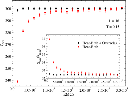
Model (1) was simulated with a mixture of heat bath and (microcanonical) overrelaxation taken from lattice QCD OVERRELAX but also effective for frustrated spin models OVERRELAXSPIN . We straightforwardly modified the implementation for $J_{ij}=1$ in VICTORAMIT . The Elementary Monte Carlo Step (EMCS) consists on a sequential heat bath sweep, followed by (the integer part of) $5L/4$ sequential overrelaxation sweeps, to let the microcanonical wave run over the system. Overrelaxation fastly evolves chirality (in $D=1$ it inverts the local chirality). One heat bath update is roughly as CPU time consuming as 7 overrelaxations. The merits of the mixed algorithm can be assessed from Fig. 1 (standard Parallel Tempering reached only $L=12$ for the same model YOUNG ). Overrelaxation may be combined with Parallel Tempering, but this is unnecessary at $T_{\mathrm{c}}$. Lattices $L=4,6,8,12,16,24$ and $32$ were simulated close to $T_{\mathrm{c}}\approx 0.16(2)$ YOUNG ; QUIRALES (see table 1). We extrapolate to nearby temperatures using bias-corrected BIAS data reweighting SPECTRALDENSITY .

Figure 1: Comparison of heat bath vs. heat bath plus overrelaxation evolution of $\chi_{\mathrm{SG}}(\vec{0})$ ( $\chi_{\mathrm{SG}}(\vec{k}_{min})$ in the inset) from a hot start (EMCS: either 1 heat bath step followed by 20 overrelaxation sweeps or 4 heat bath sweeps). Points in the plot are the average over 2500 samples of 15000 successive EMCS.

L	$4$	$6$	$8$	$12$	$16$	$24$	$32$
T	0.15	0.15	0.15	0.150	0.150	0.146	0.145
	0.16	0.16	0.155	0.155	0.156	0.150	0.147
			0.160	0.160	0.160	0.155	0.150
$N_{\mathrm{samples}}$	2	4	2	3	2.5	2	$1$
$(\times 10^{3})$	2	6	2	2.4	2.5	1.3	$1$
			2	3	2	2	$2$
EMCS$\times 10^{5}$	$1$	$1$	$1$	$2$	$3$	$16$	$40$

Table 1: Details of simulation. For each lattice size, we give the studied temperatures, the number of simulated samples (in the same order), and the number of elementary Monte Carlo steps per sample. In each sample we took $10^{5}$ measurements, excepting for $L=32$ (20000 measurements).

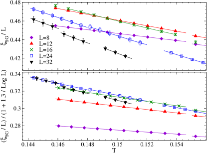
Thermalization is a major issue in SG simulations. Our thermalization tests included the by now standard $\log_{2}$ data binning (i.e. average over all samples the second half of the generated data, and compare this average with that of the second fourth of the Monte Carlo history, the average over the second eighth, and so on), finding compatibility for the last three bins. Another strong thermalization test is the consistency of the reweighting extrapolation SPECTRALDENSITY . As Fig. 3 shows, the reweighting extrapolation is satisfactory for our data. It is a nice check, because simulations at different $T$ are completely independent.

We use the quotients FSS method QUOTIENTS . The used scaling variable is $\xi_{L}/L$ FSS-PISA ; QUOTIENTS , rather than the unknown $L/\xi_{\infty}$ or $(T-T_{\mathrm{c}})L^{1/\nu}$. For an observable $O$, diverging in the large $L$ limit as $\overline{\langle O\rangle}_{J,L=\infty}\propto|T-T_{\mathrm{c}}|^{x_{O}}$, we compare $\overline{\langle O\rangle_{J}}$ in lattices $L_{1}$ and $L_{2}$, at the crossing temperature $T^{L_{1},L_{2}}$ such that $\xi_{L_{1}}(T^{L_{1},L_{2}})/L_{1}=\xi_{L_{2}}(T^{L_{1},L_{2}})/L_{2}\,$:

$$\frac{\overline{\langle O_{L_{2}}(T^{L_{1},L_{2}})\rangle_{J}}}{\overline{\langle O_{L_{1}}(T^{L_{1},L_{2}})\rangle_{J}}}=\left(\frac{L_{2}}{L_{1}}\right)^{\frac{x_{O}}{\nu}}+\ldots\,,$$ (7)

where $\nu$ is the correlation length critical exponent (the dots stand for scaling corrections VICTORAMIT ). The advantages of Eq.(7) are many QUOTIENTS ; BALLESTEROS ; BIAS ; JORG . It is easy to use. Arbitrary choices on the temperature range are avoided. The statistical error estimation is crystal clear. One directly observes scaling corrections by increasing $L_{1}$ and $L_{2}$.

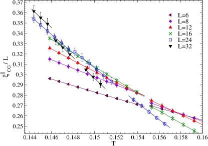
Should $T^{L_{1},L_{2}}$ be obtained from $\xi_{L,\mathrm{CG}}$ or from $\xi_{L,\mathrm{SG}}$? There is a consensus on the divergence of $\xi_{\mathrm{CG}}$ at $T_{\mathrm{c}}$, while that of $\xi_{\mathrm{SG}}$ is controversial YOUNG ; QUIRALESNEW . Moreover, $\xi_{L,\mathrm{CG}}$ suffers smaller scaling corrections (Fig. 4). So, the results in table 2 were obtained with $\xi_{L,\mathrm{CG}}$. As for $\xi_{L,\mathrm{SG}}$, we treat it here as an observable scaling as $L^{\phi}$. Some groups YOUNG ; OTROS ; FELIX expect $\phi=1$, while others QUIRALES ; QUIRALESNEW believe that $\phi=0$.

Several features are salient in table 2. (i) Once we neglect $L=4$, the $L$ evolution of our estimates is monotonic with increasing $L_{1}$ and $L_{2}$ (we agree with Refs. YOUNG ; QUIRALESNEW within their $L$ window). (ii) The $1/\nu$ from $\partial_{T}\xi_{\mathrm{SG}}$ and $\partial_{T}\xi_{\mathrm{CG}}$ is compatible for $L\geq 12$ . (iii) When $L_{1}$ and $L_{2}$ increases, $1/\nu$ systematically decreases (in a Kosterlitz-Thouless scenario it tends to zero). (iv) Exponent $\gamma_{\mathrm{SG}}/\nu$ stabilizes for $L\geq 12$ in a typical $D=3$ value QUOTIENTS , hence:

$$\chi_{\mathrm{SG}}\propto\xi_{\mathrm{CG}}^{1.93\pm 0.02}\,.$$ (8)

The scenario of Refs. QUIRALES ; QUIRALESNEW , where $\xi_{\mathrm{CG}}$ diverges at $T_{\mathrm{c}}$, while $\xi_{\mathrm{SG}}$ (and then $\chi_{\mathrm{SG}}$) does not, becomes untenable.

$L_{1}$	$L_{2}$	$\phi$	$1/\nu_{\mathrm{SG}}$	$1/\nu_{\mathrm{CG}}$	$\gamma_{\mathrm{SG}}/\nu_{\mathrm{SG}}$	$\gamma_{\mathrm{CG}}/\nu_{\mathrm{CG}}$
4	8	1.047(5)	$1.278(10)$	$1.077(20)$	$2.117(7)$	$1.061(10)$
6	12	1.057(3)	$1.223(10)$	$0.761(12)$	$2.056(5)$	$0.628(11)$
8	16	1.013(4)	$0.989(10)$	$0.722(12)$	$2.008(8)$	$0.738(18)$
12	24	0.939(4)	$0.71(17)$	$0.66(11)$	$1.954(9)$	$0.925(22)$
16	24	0.917(5)	$0.68(11)$	$0.67(12)$	$1.943(15)$	$1.02(4)$
16	32	0.908(5)	$0.72(20)$	$0.73(11)$	$1.945(13)$	$1.130(29)$
24	32A	0.88(2)	$0.60(10)$	$0.64(12)$	$1.93(2)$	$1.26(7)$
24	32B	0.91(2)	$0.56(12)$	$0.51(13)$	$1.96(4)$	$1.36(11)$

Table 2: Critical exponents from Eq.(7) ($T^{L_{1},L2}$ from $\xi_{L,\mathrm{CG}}^{\|}$). The $O$ were: $\xi_{\mathrm{SG}}$ ($\phi$: $\xi_{\mathrm{SG}}\sim L^{\phi}$), $\partial_{T}\xi_{L}/L$ ($1/\nu$) and $\chi$ ($\gamma/\nu$). The $L_{1}=24$, $L_{2}=32$ crossing is unclear (Fig. 4), so we quote results at $T^{L_{1},L_{2}}=0.146$ ($A$) and $0.145$ ($B$).

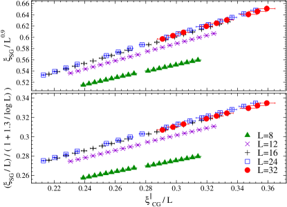
At criticality (table 2), $\xi_{\mathrm{SG}}$ scales as $L^{0.9}$ rather than $L^{1}$, immediately suggesting the presence of logarithmic corrections to scaling. Without analytical guidance, the detailed numerical study of logarithmic scaling corrections BIAS is out of reach. Thus, we borrow the leading scaling corrections from the $D=2$ XY model HASENB ($f_{\xi}$ is a smooth scaling function, while $A$ is a scaling amplitude):

$$\frac{\xi_{L,\mathrm{SG}}}{L}=f_{\xi}(\xi_{L,\mathrm{CG}}/L)\left(1+\frac{A}{\log L}+\ldots\right)\,.$$ (9)

Indeed, see Fig. 2, Eq.(9) accounts for the $L^{0.9}$ scaling ($A=1.3$, roughly 4 times that of the 2D-XY model HASENB ). One also expects HASENB multiplicative logarithms in Eq.(8). Note however that Eq.(9) works in a limited range of $L$ for any system barely above its lower critical dimension since it is the $\omega\to 0$ limit of the standard leading correction to scaling, $L^{-\omega}$ VICTORAMIT (e.g. the $2+\epsilon$ expansion 2PLUSEPS yields $\omega\approx\epsilon$ for the Heisenberg ferromagnet, whose lower critical dimension is two).

Figure 2: (color online) Top: For our largest systems $\xi_{\mathrm{SG}}$ scales as $L^{0.9}$, using $\xi_{\mathrm{CG}}/L$ as scaling variable. Bottom: The results in the upper part may be interpreted as the logarithmic corrections to scaling in Eq. (9), particularly for $L>12$.

We now study $\xi_{\mathrm{SG}}/L$ as a function of temperature (Fig.  3). If we do not correct for scaling corrections (Fig. 3, top), indeed all crossings are in the rather large range $T_{\mathrm{c}}=0.16(2)$ YOUNG ; QUIRALES . However, we observe a net shift of the crossings to lower $T$ when the system sizes grow, (for $L=24$ and $L=32$ a crossing is not found on the simulated $T$ range). Yet, Fig. 3–bottom, dividing out the logarithm scaling corrections in Eq.(9), the curves for the largest systems merge around $T=0.146$, as expected for a Kosterlitz-Thouless transition (see e.g. Ref. BALLESTEROS ).

Figure 3: (color online) Top: $\xi_{\mathrm{SG}}$ in units of $L$, versus $T$, for several lattice sizes. Lines join data obtained from a single simulation SPECTRALDENSITY (all simulations independent). For the sake of clarity we only represent data for $L\geq 8$. Bottom: as top, correcting the suspected logarithmic corrections, Eq.(9).

For the sake of completeness, let us consider our data for $\xi_{L,\mathrm{SG}}$ under the spin-chirality decoupling assumption. In this scenario, $\xi_{\infty,\mathrm{SG}}$ diverges at $T=0$, as $\xi_{\infty,\mathrm{SG}}=A/T^{\mathrm{\nu^{*}}}$ ($\nu^{*}=2.2$, according to QUIRALESNEW ). FSS VICTORAMIT predicts that $\xi_{L,\mathrm{SG}}/L$ is a smooth function of $L/\xi_{\infty,\mathrm{SG}}$. Take now from Fig. 3–top the temperature where $\xi_{L,\mathrm{SG}}/L$ reaches (say) 0.44 for $L=24$ and $L=32$, namely $T_{24}\approx 0.1508$ and $T_{32}\approx 0.1474$. In other words, $\xi_{\infty,\mathrm{SG}}$ increases a factor $32/24\approx 1.33$ while the temperature merely decreases by a $2\%$. Matching this with an algebraic divergence at $T=0$, the nonsensical result $\nu^{*}\approx 12$ is obtained.

Consider now $\xi_{\mathrm{CG}}^{\|}/L$, shown in Fig. 4. Although less than for $\xi_{\mathrm{SG}}$, the crossings shift to lower $T$ for larger $L$. For $L=8,12$ and $16$ we resolve a crossing at $T\approx 0.155$. For $L\geq 16$ the curves merge at $T\approx 0.147$, suggesting again a Kosterlitz-Thouless scaling, but with smaller scaling corrections. The $L=32$ data at low $T$ are compatible with, but above, the $L=24$ data. We suspect of a statistical fluctuation (the three $L=32$ simulations are independent), but a crossing may not be discarded.

Figure 4: (color online) Parallel chiral correlation length in units of $L$, as a function of $T$, for several lattice sizes.

In summary, we have shown that the Heisenberg spin glass undergoes a spin glass transition in $D=3$, by means of Monte Carlo simulation and FSS analysis QUOTIENTS ; BALLESTEROS ; VICTORAMIT . We have adapted a lattice gauge theory algorithm OVERRELAX , that thermalizes $L=32$ systems, well beyond any previous spin glass simulation in $D=3$. Furthermore, a large number of samples were studied in Marenostrum. For studies in the low temperature phase, we suggest to combine our algorithm with Parallel Tempering. The large range of system sizes studied allows us to conclude that, at criticality, the spin glass susceptibility scales with the chiral correlation length, Eq.(8). Therefore, a single phase transition is present in this problem: spin-chirality decoupling is ruled out. We observe logarithmic corrections to scaling, explaining why previous investigations Tc0 ; MATSUBARA ; IMAGAWA ; VILLAIN ; QUIRALES ; QUIRALESNEW ; YOUNG ; OTROS ; FELIX were inconclusive. Our results are compatible with Kosterlitz-Thouless scaling, but they are typical as well of a system with a lower critical dimension barely smaller than three.

We thank L. A. Fenández, J.J. Ruiz-Lorenzo and J.L. Alonso for discussions, and BIFI (U. Z.) and Marenostrum (Barcelona Supercomputing Center) for computing time. We were partly supported by BSCH—UCM, by DGA–Spain (M.C.-A and S.P.-G.), and by MEC (Spain) through contracts BFM2003-08532, FIS2004-05073.

References

- (1) See e.g. Spin Glasses and Random Fields, Ed. A. P. Young. World Scientific (Singapore, 1997); M. Mézard, G. Parisi and M.A. Virasoro, Spin-glass theory and beyond (World Scientific Singapore, 1987).
- (2) H. G. Ballesteros et al., Phys. Rev. B 62, 14237 (2000).
- (3) M. Palassini and S. Caracciolo, Phys. Rev. Lett. 82, 5128 (1999).
- (4) H. G. Ballesteros et al., Phys. Lett. B 378, 207 (1996); B387, 125 (1996), Nucl. Phys. B483, (1997) 707.
- (5) See, e.g., D. Amit and V. Martin-Mayor, Field Theory, the Renormalization Group and Critical Phenomena, (World-Scientific Singapore, third edition, 2005).
- (6) S. Caracciolo et al., Phys. Rev. Lett. 74, 2969 (1995).
- (7) T. Jörg, cond-mat/0602215.
- (8) H.G. Katzgraber, M. Körner and A.P. Young, cond-mat/0602212.
- (9) W.L. McMillan, Phys. Rev. B 31, 342 (1985); J.A. Olive, A.P. Young and D. Sherrington, ibid 34, 6341 (1986); B.M. Morris et al., J. Phys. C 19, 1157 (1986).
- (10) F. Matsubara, T. Iyota and S. Inawashiro, Phys. Rev. Lett. 67, 1458 (1991).
- (11) D. Imagawa and H. Kawamura, Phys. Rev. Lett. 92, 77204 (2004).
- (12) A. Mauger et al., Phys. Rev. B 41, 4587 (1990).
- (13) H. Kawamura, Phys. Rev. Lett. 80, 5421 (1998); K. Hukushima and H. Kawamura, Phys. Rev. E 61, R1008 (2000).
- (14) K. Hukushima and H. Kawamura, Phys. Rev. B 72, 144416 (2005).
- (15) L.W. Lee and A.P. Young, Phys. Rev. Lett. 90, 227203 (2003).
- (16) F. Matsubara, T. Shirakura and S. Endoh, Phys. Rev. B 64, 092412 (2001); T. Nakamura and S. Endoh, J. Phys. Soc. Jpn. 71, 2113 (2002).
- (17) M. Picco and F. Ritort, Phys. Rev. B 71, 100406 (2005).
- (18) F. Bert et al., Phys. Rev. Lett. 92, 167203 (2004).
- (19) D. Petit, L. Fruchter and I.A. Campbell, Phys. Rev. Lett. 83, 5130 (1999); 88, 207206 (2002).
- (20) F. Cooper, B. Freedman and D. Preston, Nucl. Phys. B 210, 210 (1982).
- (21) F. R. Brown and T. J. Woch, Phys. Rev. Lett. 58, 2394 (1987).
- (22) J.M. Kosterlitz and D.J. Thouless, J. Phys. C 6, 1181 (1973).
- (23) J. L. Alonso et al., Phys. Rev. B 53 (1996) 2537; E. Marinari, V. Martin-Mayor and A. Pagnani, ibid 62 (2000) 4999.
- (24) M. Falcioni et al., Phys. Lett. B 108, 331 (1982); A. M. Ferrenberg and R. H. Swendsen, Phys. Rev. Lett. 61, 2635 (1988).
- (25) H. G. Ballesteros et al., Nucl. Phys. B 512, 681 (1998).
- (26) M. Hasenbusch, J.Phys. A 38, 5869 (2005).
- (27) A.M. Polyakov, Phys. Lett. B 59, 79 (1975); E. Brèzin and J. Zinn-Justin, Phys. Rev. B 14, 3110 (1976).