Fermi liquid theory for heavy fermion superconductors without inversion symmetry : Magnetism and transport coefficients

Abstract

We present the microscopic Fermi liquid theory for magnetic properties and transport phenomena in interacting electron systems without inversion symmetry both in the normal state and in the superconducting state. Our argument is mainly focused on the application to noncentrosymmetric heavy fermion superconductors. The transport coefficients for the anomalous Hall effect, the thermal anomalous Hall effect, the spin Hall effect, and magnetoelectric effects, of which the existence is a remarkable feature of parity violation, are obtained by taking into account electron correlation effects in a formally exact way. Moreover, we demonstrate that the temperature dependence of the spin susceptibility which consists of the Pauli term and van-Vleck-like term seriously depends on the details of the electronic structure. We give a possible explanation for the recent experimental result obtained by the NMR measurement of CePt₃Si [Yogi et al.: J. Phys. Soc. Jpn.75 (2006) 013709], which indicates no change of the Knight shift below the superconducting transition temperature for any directions of a magnetic field.

I Introduction

For a large class of superconductors, there exists inversion symmetry which allows the classification of the Cooper pair according to parity; i.e. a spin singlet or triplet pairing state realizes. This idea is not applicable to the recently discovered noncentrosymmetric superconductors, CePt₃Si, UIr, CeRhSi₃, CeIrSi₃, and Li₂(Pd_1-xPt_x)B.bau ; uir ; kim ; onuki ; tog1 ; tog2 In systems without inversion center, parity violation yields the admixture of the spin singlet and triplet pairing states, as pointed out by Edelstein nearly two decades ago.ede1 ; gor An asymmetric potential gradient $\nabla V$ caused by the absence of inversion symmetry gives rise to the spin-orbit interaction $\alpha(\mbox{\boldmath$k$}\times\nabla V)\cdot\mbox{\boldmath$\sigma$}$ which splits the Fermi surface into two pieces and aligns electron spins on each Fermi surfaces parallel to $\mbox{\boldmath$k$}_{F}\times\nabla V$, with $\mbox{\boldmath$k$}_{F}$ the Fermi momentum. A simple example of this situation for the Rashba type spin-orbit interaction with $\nabla V$ parallel to the $z$-axis is depicted in FIG.1. Note that in FIG.1 the spin quantization axis is chosen along $\mbox{\boldmath$k$}_{F}\times\nabla V$. On one of the spin-orbit splitted Fermi surfaces, say the $(+)$-band in FIG.1, the Cooper pair between electrons with momentum $k$, spin $\uparrow$ and momentum $-k$, spin $\downarrow$ is formed. This state, denoted as $|k\uparrow\rangle|-k\downarrow\rangle$, is not a spin singlet state, because the counterpart of this state $|k\downarrow\rangle|-k\uparrow\rangle$ is formed on another Fermi surface and thus the superposition between these two states is not possible. Actually, the pairing state $|k\uparrow\rangle|-k\downarrow\rangle$ is the admixture of spin singlet and triplet states as easily verified by,

$$|k\uparrow\rangle|-k\downarrow\rangle = \frac{1}{2}(|k\uparrow\rangle|-k\downarrow\rangle-|k\downarrow\rangle|-k\uparrow\rangle)$$

$$+ \frac{1}{2}(|k\uparrow\rangle|-k\downarrow\rangle+|k\downarrow\rangle|-k\uparrow\rangle).$$

The first and second terms of the right-hand side express, respectively, a spin singlet state and a spin triplet state with the in-plane spin projection $S_{\rm inplane}$ equal to $0$. Since we take the spin quantization axis parallel to the $xy$-plane, this triplet state corresponds to the $S^{z}=\pm 1$ state for the spin quantization axis along the $z$-direction. (This means that the $\vec{d}$-vector of the triplet component is parallel to the plane.) The above explanation is also applicable to general cases with more complicated form of $\nabla V$. This unique superconducting state exhibits various interesting electromagnetic properties as extensively argued by many authors.ede1 ; gor ; fri ; ser ; ede2 ; yip ; yip2 ; sam2 ; kau ; fuji2 ; haya ; tana ; ichi

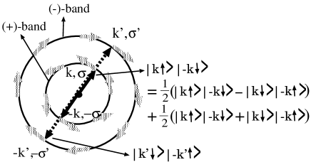
Figure 1: An example of two-dimensional Fermi surfaces splitted by the Rashba spin-orbit interaction depicted on the $k_{x}$-$k_{y}$ plane. The inversion symmetry is broken along the $z$-direction. The gray arrows represent electron spins on the Fermi surfaces for the $(+)$-band and the $(-)$-band. The Cooper pairs between electrons with momentum $k$, spin $\sigma$ and momentum $-k$, spin $-\sigma$ are formed on each Fermi surfaces.

In addition to the superconducting state, the absence of inversion symmetry also affects properties of the normal state in a drastic way. One remarkable feature appears in paramagnetic effects; i.e. there is a van-Vleck-like spin susceptibility due to the transition between the spin-orbit splitted Fermi surfaces.ede1 ; gor ; fri This effect should be distinguished from the usual van Vleck term of the orbital susceptibility by the fact that in contrast to the usual van Vleck term, the van-Vleck-like susceptibility in inversion-symmetry-broken systems varies as a function of temperature like the Pauli susceptibility. The existence of the van-Vleck-like term is crucial for experimental investigations on superconducting states because it exhibits no change even below the superconducting transition temperature $T_{c}$ for both the spin-singlet and triplet states when the spin-orbit splitting is sufficiently larger than the superconducting gap.gor ; fri For the determination of the symmetry of the Cooper pair, we need precise knowledge about the behaviors of the van-Vleck-like susceptibility both below and above $T_{c}$.

Furthermore, the parity-breaking spin-orbit interaction gives rise to nontrivial coupling between charge and spin degrees of freedom, and thus causes unique transport properties. For example, there exist magnetoelectric effects such as the electric-field-induced magnetization,lev ; ede0 and the spin Hall effect which is characterized by the transverse spin current caused by an electric field.she ; she2 Also, the anomalous Hall effect considered by Karplus and Luttinger five decades ago is possible to occur.kl For heavy fermion systems without inversion symmetry, the experimental studies on these effects are important future issues.

In the heavy fermion superconductors CePt₃Si, CeRhSi₃, UIr, and CeIrSi₃, strong electron correlation which yields an extremely enhanced effective electron mass plays a crucial role. For the clarification of the nature of these systems, it is important to understand effects of the electron correlation on the aforementioned exotic phenomena. The main part of this paper is devoted to this purpose. On the basis of a general framework of the Fermi liquid theory, we derive the formulae for the spin susceptibility and the transport coefficients related to the anomalous Hall effect, the thermal anomalous Hall effect, the spin Hall effect and the magnetoelectric effect taking into account strong electron correlation effects in a formally exact way. Using these formulae, we argue how strong electron correlation inherent in heavy fermion systems affect experimentally observable quantities. The insights obtained from this analysis are useful for the exploration of the superconducting state realized in CePt₃Si, CeRhSi₃, and CeIrSi₃, as explained below.

The main results of this paper are summarized as follows:

(i) The thermal anomalous Hall effect, which is the anomalous Hall effect for the heat current is predominated by the contributions from electrons away from the Fermi surface. It implies that when the spin-orbit splitting is much larger than the superconducting gap, the behavior of the thermal anomalous Hall conductivity $\kappa^{\rm AHE}_{xy}$ in the superconducting state is similar to that in the normal state. Even in the zero temperature limit $T\rightarrow 0$, $\kappa^{\rm AHE}/TH_{z}$ with $H_{z}$ an applied magnetic field is finite, and much enhanced by electron correlation effects in heavy fermion systems.

(ii) In the Rashba case where the inversion symmetry is broken along the $z$-direction, as in the case of CePt₃Si, CeRhSi₃, and CeIrSi₃, the spin Hall conductivity, which is given by the correlation function between a charge current and a transverse spin current, is not at all affected by electron correlation effects, but determined only by the band structure.

(iii) We clarify electron correlation effects on the magnetoelectric effect both in the normal state and in the superconducting state. As was considered by Levitov et al.,lev in the normal state, the bulk magnetization is induced by an applied electric field, $M=\Upsilon E$, and, conversely, the charge current flow is induced by an AC magnetic field, $J=-\Upsilon\dot{B}$. We find that in the temperature region where the resistivity exhibits $T^{2}$-dependence, the magnetoelectric effect coefficient $\Upsilon$ behaves like $\sim 1/(\gamma T^{2})$, with $\gamma$ the specific heat coefficient, while in the temperature region where the resistivity is dominated by impurity scattering, $\Upsilon$ is enhanced by a factor $\sim\gamma$. In the superconducting state, the paramagnetic supercurrent is generated by the Zeeman field, as extensively argued by several authors.ede1 ; ede2 ; yip ; fuji2 We reveal electron correlation effects on this supercurrent from a general theoretical framework.

(iv) The temperature dependence of the van-Vleck-like spin susceptibility $\chi^{\rm VV}(T)$ crucially depends on the details of the electronic structure, and occasionally may become stronger than that of the Pauli susceptibility $\chi^{\rm Pauli}(T)$, in contrast to the usual van Vleck orbital susceptibility, which is independent of temperatures. Also, in the superconducting state, the ratio of $\chi^{\rm VV}(T)$ to the total spin susceptibility $\chi(T)=\chi^{\rm Pauli}(T)+\chi^{\rm VV}(T)$ in the zero temperature limit is seriously affected by both the electronic structure and electron correlation effects. This result yields an important implication for the recent NMR measurements for CePt₃Si carried out by Yogi et al.,yogi ; yogi2 which indicate no change of the Knight shift below $T_{c}$ for any directions of an applied magnetic field, contrary to the previous theoretical prediction that for a magnetic field along the $z$-axis, $\chi(0)=\chi(T_{c})/2$ for a sufficiently strong spin-orbit coupling. Our precise analysis indicates that for a specific electronic structure, $\chi(T)$ is dominated by $\chi^{\rm VV}$, and as a result, $\chi(0)\approx\chi(T_{c})$, which is consistent with the aforementioned NMR experiment.

The organization of this paper is as follows. In the next section, we develop the analysis for the normal state, exploring the static magnetic properties and the transport coefficients. In the section III, we extend our approach to the superconducting with particular emphasis on the magnetism. We propose a possible explanation for the recent NMR experimental data. We also argue electron correlation effects on the paramagnetic supercurrent caused by the inversion-symmetry-breaking spin-orbit interaction. A summary is given in the section IV.

II Normal state

II.1 Basic equations

In this section, we consider a single band interacting electron model with a lattice structure breaking inversion symmetry. An extension to more complicated systems such as the periodic Anderson model is straightforward, and will be discussed elsewhere. Our model Hamiltonian is given by,

$$\mathcal{H} = \mathcal{H}_{0}+\mathcal{H}_{\rm SO},$$ (1)

$$\mathcal{H}_{0} = \sum_{k,\sigma}\varepsilon_{k}c^{\dagger}_{k}c_{k}+U\sum_{i}n_{\uparrow i}n_{\downarrow i},$$ (2)

$$\mathcal{H}_{\rm SO} = \alpha\sum_{k}c^{\dagger}_{k}\mbox{\boldmath$\mathcal{L}$}_{0}(k)\cdot\mbox{\boldmath$\sigma$}c_{k},$$ (3)

where $c^{\dagger}_{k}=(c^{\dagger}_{\uparrow k},c^{\dagger}_{\downarrow k})$ is the two-component spinor field for an electron with spin $\uparrow$, $\downarrow$, and momentum $k$. $n_{\sigma i}=c^{\dagger}_{\sigma i}c_{\sigma i}$ is the number density operator at the site $i$. $\mbox{\boldmath$\sigma$}=(\sigma_{x},\sigma_{y},\sigma_{z})$ with $\sigma_{\nu}$, $\nu=x,y,z$, the Pauli matrix. For simplicity, we have assumed the on-site Coulomb repulsion with the coupling constant $U$ in Eq.(2). The vector $\mbox{\boldmath$\mathcal{L}$}_{0}(k)=({\cal L}_{0x},{\cal L}_{0y},{\cal L}_{0z})$ in the spin-orbit interaction term $\mathcal{H}_{\rm SO}$ obeys $\mbox{\boldmath$\mathcal{L}$}_{0}(-k)=-\mbox{\boldmath$\mathcal{L}$}_{0}(k)$, of which the explicit expression is determined by the detail of the crystal structure which breaks the inversion symmetry. For the tetragonal symmetry and small $k$, $\mbox{\boldmath$\mathcal{L}$}_{0}(k)=(k_{y},-k_{x},0)$ which leads the Rashba-type spin-orbit interaction.ras For the cubic symmetry with Zinc Blende structures and small $k$, $\mbox{\boldmath$\mathcal{L}$}_{0}(k)=(k_{x}(k_{y}^{2}-k_{z}^{2}),k_{y}(k_{z}^{2}-k_{x}^{2}),k_{z}(k_{x}^{2}-k_{y}^{2}))$, which is related to the Dresselhaus spin-orbit interaction.dres ; dyp ; sil

In the following, we are concerned with magnetic properties of the system. Unique features of magnetism in inversion-symmetry-broken systems appear as a result of paramagnetic effects rather than diamagnetic effects. Thus we add to the Hamiltonian (1) the Zeeman coupling with an external magnetic field $\mbox{\boldmath$H$}=(H_{x},H_{y},H_{z})$,

$$H_{\rm Zeeman}=\sum_{k}c^{\dagger}_{k}\mu_{\rm B}\mbox{\boldmath$\sigma$}\cdot\mbox{\boldmath$H$}c_{k},$$ (4)

and neglect the orbital diamagnetic effects. For simplicity, we assume that the $g$-value is equal to 2. Then, the inverse of the single-particle Green’s function under the applied magnetic field is defined as,

$$\hat{G}^{-1}(p)=i\varepsilon_{n}-\hat{H}(p)+\mu_{\rm B}\mbox{\boldmath$\sigma$}\cdot\mbox{\boldmath$H$},$$ (5)

where $p=(i\varepsilon_{n},\mbox{\boldmath$k$})$, and,

$$\hat{H}(p)=\hat{H}_{0}(p)+\hat{\Sigma}(p),$$ (6)

$$\hat{H}_{0}=\varepsilon_{k}-\mu+\alpha\mbox{\boldmath$\mathcal{L}$}_{0}(k)\cdot\mbox{\boldmath$\sigma$}$$ (7)

with $\mu$ the chemical potential. The self-energy matrix $\hat{\Sigma}$ consists of both diagonal and off-diagonal components,

$$\hat{\Sigma} = \left(\begin{array}[]{cc}\Sigma_{\uparrow\uparrow}(p)&\Sigma_{\uparrow\downarrow}(p)\\ \Sigma_{\downarrow\uparrow}(p)&\Sigma_{\downarrow\downarrow}(p)\end{array}\right)$$ (10)

$$= \Sigma_{0}+\mbox{\boldmath$\Sigma$}\cdot\mbox{\boldmath$\sigma$}.$$ (11)

Here $\mbox{\boldmath$\Sigma$}=(\Sigma_{x},\Sigma_{y},\Sigma_{z})$ with $\Sigma_{0}=(\Sigma_{\uparrow\uparrow}+\Sigma_{\downarrow\downarrow})/2$, $\Sigma_{x}=(\Sigma_{\downarrow\uparrow}+\Sigma_{\uparrow\downarrow})/2$, $\Sigma_{y}=(\Sigma_{\downarrow\uparrow}-\Sigma_{\uparrow\downarrow})/2i$, and $\Sigma_{z}=(\Sigma_{\uparrow\uparrow}-\Sigma_{\downarrow\downarrow})/2$.

It is convenient to introduce a vectorial function,

$$\mbox{\boldmath$\mathcal{L}$}(p)=({\cal L}_{x}(p),{\cal L}_{y}(p),{\cal L}_{z}(p))=\mbox{\boldmath$\mathcal{L}$}_{0}(k)-\frac{\mu_{\rm B}}{\alpha}\mbox{\boldmath$H$}+\frac{1}{\alpha}\mbox{\boldmath$\Sigma$}(p).$$ (12)

Generally, $\mbox{\boldmath$\mathcal{L}$}(p)$ is non-Hermitian, because $\Sigma_{x}$ and $\Sigma_{y}$ may be complex quantities. However, $\hat{G}^{-1}(p)=i\varepsilon-\varepsilon_{k}+\mu-\Sigma_{0}(p)-\alpha\mbox{\boldmath$\mathcal{L}$}(p)\cdot\mbox{\boldmath$\sigma$}$ is diagonalized by the transformation $\hat{U}(p)\hat{G}^{-1}(p)\hat{U}_{+}(p)$ with,

$$\hat{U}(p)=\left(\begin{array}[]{cc}\xi_{+}(p)&\xi_{-}(p)\eta_{-}(p)\\ -\xi_{-}(p)\eta_{+}(p)&\xi_{+}(p)\end{array}\right),$$ (15)

$$\hat{U}_{+}(p)=\left(\begin{array}[]{cc}\xi_{+}(p)&-\xi_{-}(p)\eta_{-}(p)\\ \xi_{-}(p)\eta_{+}(p)&\xi_{+}(p)\end{array}\right),$$ (18)

$$\xi_{\pm}(p)=\frac{1}{\sqrt{2}}\left[1\pm\frac{{\cal L}_{z}(p)}{\|\mbox{\boldmath$\mathcal{L}$}(p)\|}\right]^{\frac{1}{2}},$$ (19)

$$\eta_{\pm}(p)=\frac{{\cal L}_{x}(p)\pm i{\cal L}_{y}(p)}{\sqrt{{{\cal L}_{x}(p)}^{2}+{{\cal L}_{y}(p)}^{2}}}.$$ (20)

Here $\|\mbox{\boldmath$\mathcal{L}$}(p)\|=\sqrt{\mathcal{L}_{x}^{2}+\mathcal{L}_{y}^{2}+\mathcal{L}_{z}^{2}}$. In the absence of the magnetic field, we can verify that the time reversal symmetry leads the relation

$$\Sigma_{\uparrow\downarrow}^{*}(z,-\mbox{\boldmath$k$})=-\Sigma_{\downarrow\uparrow}(z,\mbox{\boldmath$k$}).$$ (21)

As seen from eqs.(6),(7), and (11), the main effect of the off-diagonal self-energy terms, $\Sigma_{\uparrow\downarrow}$, $\Sigma_{\downarrow\uparrow}$ is to renormalize the spin-orbit interaction term. Since the on-site Coulomb interaction does not change the symmetry of the system, the off-diagonal self-energy should obey the same symmetric properties as $\mbox{\boldmath$\mathcal{L}$}_{0}(k)$ in the absence of magnetic fields; i.e.

$$\mbox{\boldmath$\Sigma$}(i\varepsilon_{n},-\mbox{\boldmath$k$})=-\mbox{\boldmath$\Sigma$}(i\varepsilon_{n},\mbox{\boldmath$k$}).$$ (22)

In particular, for the Rashba interaction,

$$\Sigma_{x}(k_{x},-k_{y})=-\Sigma_{x}(k_{x},k_{y}),$$ (23)

$$\Sigma_{y}(-k_{x},k_{y})=-\Sigma_{y}(k_{x},k_{y}),$$ (24)

and $\Sigma_{x}$ ($\Sigma_{y}$) is an even function of $k_{x}$ ($k_{y}$).

The relations (21) and (22) imply that when the time reversal symmetry is preserved, $\Sigma_{x}$ and $\Sigma_{y}$ are real quantities, and thus $\hat{U}(p)$ is unitary, i.e. $\hat{U}_{+}(p)=\hat{U}^{\dagger}(p)$. In more general cases with $\mbox{\boldmath$H$}\neq 0$, as long as the spin-orbit splitting is much smaller than the Fermi energy, as in the case of any heavy fermion systems without inversion symmetry, the off-diagonal terms of $\hat{\Sigma}$ may be negligible compared to the diagonal terms, and $\hat{U}_{+}$ is safely approximated by $\hat{U}^{\dagger}$.

The single-particle excitation energy $\varepsilon_{k\tau}^{*}$ for the quasi-particle with the helicity $\tau=\pm 1$ is given by the solution of the equation ${\rm Det}[\hat{G}^{-1}(\varepsilon^{*}_{k\tau},\mbox{\boldmath$k$})]=0$, which is, in the diagonalized representation,

$$\varepsilon_{k\tau}^{*}+\mu-\varepsilon_{k}-\Sigma_{0}(\varepsilon_{\tau}^{*},\mbox{\boldmath$k$})-\tau\alpha\|\mbox{\boldmath$\mathcal{L}$}(\varepsilon_{k\tau}^{*},\mbox{\boldmath$k$})\|=0.$$ (25)

Using the transformation $\hat{U}(p)$, we can easily obtain the inverse of Eq.(5),

$$\hat{G}(p)=\sum_{\tau=\pm 1}\frac{1+\tau\hat{\mbox{\boldmath$\mathcal{L}$}}(p)\cdot\mbox{\boldmath$\sigma$}}{2}G_{\tau}(p),$$ (26)

where $\hat{\mbox{\boldmath$\mathcal{L}$}}(p)=\mbox{\boldmath$\mathcal{L}$}(p)/\|\mbox{\boldmath$\mathcal{L}$}(p)\|$, and

$$G_{\tau}(p)=\frac{1}{i\varepsilon_{n}-\varepsilon_{k}+\mu-\Sigma_{0}(p)-\tau\alpha\|\mbox{\boldmath$\mathcal{L}$}(p)\|}.$$ (27)

In the vicinity of the Fermi surface, the quasiparticle approximation is applicable, and the Green function for $\mbox{\boldmath$H$}=0$ is reduced to,

$$\hat{G}(p)=\sum_{\tau=\pm 1}\frac{1+\tau\hat{\mbox{\boldmath$\mathcal{L}$}}(\varepsilon_{k\tau}^{*},\mbox{\boldmath$k$})\cdot\mbox{\boldmath$\sigma$}}{2}G_{\tau}(p),$$ (28)

with

$$G_{\tau}(p)=\frac{z_{k\tau}}{i\varepsilon_{n}+i\gamma_{k\tau}{\rm sgn}\varepsilon_{n}-\varepsilon_{k\tau}^{*}}$$ (29)

Here $\gamma_{k\tau}$ is the quasi-particle damping given by

$$\gamma_{k\tau}=z_{k\tau}({\rm Im}\Sigma_{0}^{R}(\varepsilon,\mbox{\boldmath$k$})+\alpha{\rm Re}\hat{\mbox{\boldmath$\mathcal{L}$}}^{R}\cdot{\rm Im}\mbox{\boldmath$\Sigma$}^{R}(\varepsilon,\mbox{\boldmath$k$}))|_{\varepsilon\rightarrow i\varepsilon_{n}},$$ (30)

where ${\rm Re}\hat{\mbox{\boldmath$\mathcal{L}$}}^{R}={\rm Re}\mbox{\boldmath$\mathcal{L}$}^{R}(\varepsilon,\mbox{\boldmath$k$})/|{\rm Re}\mbox{\boldmath$\mathcal{L}$}^{R}(\varepsilon,\mbox{\boldmath$k$})|$ and quantities with the superscript $R$ indicates retarded functions obtained by the analytic continuation $i\varepsilon_{n}\rightarrow\varepsilon+i\delta$ ($\delta>0$). The mass renormalization factor $z_{k\tau}$ is

$$z_{k\tau}=\biggl{[}1-\frac{\partial\Sigma_{0}(p)}{\partial(i\varepsilon_{n})}-\tau\alpha\frac{\partial\|\mbox{\boldmath$\mathcal{L}$}(p)\|}{\partial(i\varepsilon_{n})}\biggr{]}^{-1}\biggr{|}_{i\varepsilon_{n}\rightarrow\varepsilon^{*}_{k\tau}}.$$ (31)

In particular, in the case of the Rashba interaction with a potential gradient along $\mbox{\boldmath$n$}=(0,0,1)$,

$$z_{k\tau} = \biggl{[}1-\frac{\partial\Sigma_{0}(p)}{\partial(i\varepsilon_{n})}-\tau\biggl{(}\hat{t}_{y}\frac{\partial\Sigma_{x}(p)}{\partial(i\varepsilon_{n})}$$ (32)

$$- \hat{t}_{x}\frac{\partial\Sigma_{y}(p)}{\partial(i\varepsilon_{n})}\biggr{)}\biggr{]}^{-1}\biggr{|}_{i\varepsilon_{n}\rightarrow\varepsilon^{*}_{k\tau}},$$

with a two-dimensional vector $\hat{\mbox{\boldmath$t$}}(p)=\mbox{\boldmath$t$}(p)/\|\mbox{\boldmath$t$}(p)\|$, $\mbox{\boldmath$t$}(p)=\mbox{\boldmath$n$}\times\mbox{\boldmath{$\mathcal{L}$}}(p)$, and $\|\mbox{\boldmath$t$}(p)\|=\sqrt{t_{x}^{2}+t_{y}^{2}}$. In the derivation of Eqs.(30), (31), and (32), it is assumed that the quasiparticle damping is sufficiently small to stabilize the Fermi liquid state; i.e. ${\rm Im}\Sigma_{\mu}^{R}(\varepsilon,\mbox{\boldmath$k$})\ll\varepsilon$ with $\mu=0,x,y,z$. We would like to stress that the notations $\Sigma_{x,y}$ is more convenient than the notations $\Sigma_{\uparrow\downarrow}$ and $\Sigma_{\downarrow\uparrow}$, because ${\rm Im}\Sigma^{R}_{\uparrow\downarrow}$ and ${\rm Im}\Sigma^{R}_{\downarrow\uparrow}$ are not directly related to the quasiparticle damping, and can not be assumed to be small.

II.2 Ward identities

In the following sections, we will argue transport phenomena and magnetic properties. In the derivation of transport coefficients, the Ward identities which relate three-point vertices of multipoint correlation functions to the single-particle Green function play a crucial role. These identity relations are derived from the conservation laws for charge and spin degrees of freedom.

The Ward identity corresponding to the charge conservation law has the standard form,

$$\sum_{\mu=0,x,y,z}q_{\mu}\Lambda^{c}_{\mu}(p+q,p)=\hat{G}^{-1}(p)-\hat{G}^{-1}(p+q),$$ (33)

where $q_{\mu}=(-i\omega,\mbox{\boldmath$q$})$, and each components of $\Lambda^{c}_{\mu}$ are the three-point vertex functions dressed by electron-electron interaction for the charge density ($\mu=0$) and the charge current ($\mu=x,y,z$) In the limit of $q\rightarrow 0$, the charge current vertex function is given by,

$$\Lambda^{c}_{\mu}(p,p)=\frac{\partial}{\partial k_{\mu}}(\varepsilon_{k}+\Sigma_{0}+\alpha(\mbox{\boldmath$\sigma$}\cdot\mbox{\boldmath$\mathcal{L}$}(p))).$$ (34)

In contrast to Eq.(33), the Ward identity for the spin degrees of freedom is affected by the spin-orbit interaction which breaks the conservation of the local spin density. To derive the Ward identity for the spin degrees of freedom, we start from the continuity equation for the spin density,

$$\frac{\partial S^{\nu}(x)}{\partial t}+\nabla\cdot\mbox{\boldmath$J$}^{s\nu}(x)=\rho_{\rm S}^{\nu}(x).$$ (35)

Here, in terms of the spinor field $\psi^{\dagger}(x)=\frac{1}{\sqrt{V}}\sum_{k}c_{k}^{\dagger}\exp(-ikx)$, the $\nu$-component of the spin density operator $S^{\nu}(x)$ ($\nu=x,y,z$) and the corresponding spin current density operator $J^{s\nu}(x)$ are expressed as,

$$S^{\nu}(x)=\psi^{\dagger}(x)\frac{\sigma_{\nu}}{2}\psi(x),$$ (36)

$$\mbox{\boldmath$J$}^{s\nu}=\frac{1}{4i}[\psi^{\dagger}(x)\sigma_{\nu}\nabla\psi(x)-\{\nabla\psi^{\dagger}(x)\}\sigma_{\nu}\psi(x)].$$ (37)

In (35), $\rho_{\rm S}^{\nu}(x)$ is the source term caused by the spin-orbit interaction $\mathcal{H}_{\rm SO}$. From the coordinate representation of $\mathcal{H}_{\rm SO}$,

$${\cal H}_{\rm SO} = \alpha\int\frac{dx}{2}[\psi^{\dagger}(x)\mbox{\boldmath$\sigma$}\cdot\{\mbox{\boldmath$\mathcal{L}$}_{0}(-i\nabla)\psi(x)\}$$ (38)

$$- \{\mbox{\boldmath$\mathcal{L}$}_{0}(-i\nabla)\psi^{\dagger}(x)\}\cdot\mbox{\boldmath$\sigma$}\psi(x)],$$

we have the explicit form of $\rho_{\rm S}^{\nu}(x)$,

$$\rho_{\rm S}^{\nu}(x) = \frac{\alpha}{2}[\psi^{\dagger}(x)\mbox{\boldmath$\sigma$}\cdot(\mbox{\boldmath$n$}_{\nu}\times\mbox{\boldmath{$\mathcal{L}$}}_{0}(-i\nabla))\psi(x)$$ (39)

$$- \{(\mbox{\boldmath$n$}_{\nu}\times\mbox{\boldmath{$\mathcal{L}$}}_{0}(-i\nabla))\cdot\mbox{\boldmath$\sigma$}\psi^{\dagger}(x)\}\psi(x)$$

$$- \psi^{\dagger}(x)i\mathcal{L}_{0\nu}(-i\nabla)\psi(x)$$

$$- i\{\mathcal{L}_{0\nu}(-i\nabla)\psi^{\dagger}(x)\}\psi(x)],$$

where $\mbox{\boldmath$n$}_{\nu}$ is a unit vector along the $\nu$-axis. In the case of the Rashba spin-orbit interaction which breaks the inversion symmetry in the $(0,0,1)$-direction, $\mbox{\boldmath{$\mathcal{L}$}}_{0}(k)=\mbox{\boldmath$t$}_{0}(k)\times\mbox{\boldmath$n$}_{z}$. Here the vector $\mbox{\boldmath$t$}_{0}(k)=(t_{0x},t_{0y},0)$ transforms like $(k_{x},k_{y},0)$. Then, the source term for $S^{z}$ is of the form,

$$\rho_{\rm S}^{z}(x) = -\frac{\alpha}{2}[\psi^{\dagger}(x)\mbox{\boldmath$\sigma$}\cdot\mbox{\boldmath$t$}_{0}(-i\nabla)\psi(x)$$ (40)

$$-\{\mbox{\boldmath$t$}_{0}(-i\nabla)\psi^{\dagger}(x)\}\cdot\mbox{\boldmath$\sigma$}\psi(x)],$$

and for $S^{x}$,

$$\rho^{x}_{S}(x) = -\frac{\alpha}{2}[\psi^{\dagger}\sigma_{z}t_{0x}(-i\nabla)\psi(x)-\{t_{0x}(-i\nabla)\psi^{\dagger}(x)\}\sigma_{z}\psi(x)$$ (41)

$$+ \psi^{\dagger}(x)it_{0y}(-i\nabla)\psi(x)+i\{t_{0y}(-i\nabla)\psi^{\dagger}(x)\}\psi(x)].$$

The standard argument applied to the continuity equation (35) leads the Ward identity for the spin degrees of freedom,sch

$$\sum_{\mu=0,x,y,z}q_{\mu}\hat{\Lambda}^{s\nu}_{\mu}(p+q,p) = \frac{\sigma_{\nu}}{2}\hat{G}^{-1}(p)-\hat{G}^{-1}(p+q)\frac{\sigma_{\nu}}{2}$$ (42)

$$+\hat{\mathcal{T}}^{\nu}(p+q,p),$$

where $\hat{\Lambda}^{s\nu}_{\mu}(p+q,p)$ ($\mu=0,x,y,z$) are the three-point vertex functions dressed by electron-electron interaction for the $\nu$-component of the spin density ($\mu=0$) and the corresponding spin current density ($\mu=x,y,z$). $\hat{\mathcal{T}}^{\nu}(p+q,p)$ is the dressed three-point vertex function for the spin source $\rho_{\rm S}^{\nu}$. $\hat{\Lambda}^{s\nu}_{\mu}$ and $\hat{\mathcal{T}}^{\nu}$ are the $2\times 2$ matrices in the spin space. The three-point vertex $\hat{\mathcal{T}}^{\nu}(p+q,p)$ is given by the solution of the following integral equation.

$$\hat{\mathcal{T}}^{\nu}(p+\frac{q}{2},p-\frac{q}{2})=\hat{\mathcal{T}}_{0}^{\nu}(p+\frac{q}{2},p-\frac{q}{2})$$

$$+\sum_{p^{\prime}}{\rm tr}[\hat{\Gamma}(p+\frac{q}{2},p-\frac{q}{2};p^{\prime}+\frac{q}{2},p^{\prime}-\frac{q}{2})$$

$$\times\hat{G}(p^{\prime}+\frac{q}{2})\hat{\mathcal{T}}^{\nu}(p^{\prime}+\frac{q}{2},p^{\prime}-\frac{q}{2})\hat{G}(p^{\prime}-\frac{q}{2})].$$ (43)

Here $\hat{\Gamma}(p_{1},p_{2};p_{3},p_{4})$ is the four-point vertex function which is irreducible with respect to particle-hole pairs. The diagrammatic representation of $\hat{\Gamma}$ with spin indices is shown in FIG.2. The bare vertex function $\hat{\mathcal{T}}_{0}^{\nu}$ is defined as

$$\hat{\mathcal{T}}_{0}^{\nu}(p+\frac{q}{2},p-\frac{q}{2})=\frac{\alpha}{2}[\mathcal{L}_{0\nu}(\mbox{\boldmath$k$}-\frac{\mbox{\boldmath$q$}}{2})-\mathcal{L}_{0\nu}(\mbox{\boldmath$k$}+\frac{\mbox{\boldmath$q$}}{2})]$$

$$+\frac{i\alpha}{2}(\{\mbox{\boldmath$\mathcal{L}$}_{0}(\mbox{\boldmath$k$}+\frac{\mbox{\boldmath$q$}}{2})+\mbox{\boldmath$\mathcal{L}$}_{0}(\mbox{\boldmath$k$}-\frac{\mbox{\boldmath$q$}}{2})\}\times\mbox{\boldmath$\sigma$})\cdot\mbox{\boldmath$n$}_{\nu}.$$ (44)

In the case of the Rashba spin-orbit interaction, the $z$-component of the bare vertex function is,

$$\hat{\mathcal{T}}_{0}^{z}(\mbox{\boldmath$k$}+\frac{\mbox{\boldmath$q$}}{2},\mbox{\boldmath$k$}-\frac{\mbox{\boldmath$q$}}{2})=\frac{i\alpha}{2}\mbox{\boldmath$\sigma$}\cdot[\mbox{\boldmath$t$}_{0}(\mbox{\boldmath$k$}+\frac{\mbox{\boldmath$q$}}{2})+\mbox{\boldmath$t$}_{0}(\mbox{\boldmath$k$}-\frac{\mbox{\boldmath$q$}}{2})],$$ (45)

and the $x$-component is,

$$\hat{\mathcal{T}}_{0}^{x}(\mbox{\boldmath$k$}+\frac{\mbox{\boldmath$q$}}{2},\mbox{\boldmath$k$}-\frac{\mbox{\boldmath$q$}}{2})=-\frac{\alpha}{2}[t_{0y}(\mbox{\boldmath$k$}+\frac{\mbox{\boldmath$q$}}{2})-t_{0y}(\mbox{\boldmath$k$}-\frac{\mbox{\boldmath$q$}}{2})]$$

$$-\frac{i\alpha\sigma_{z}}{2}[t_{0x}(\mbox{\boldmath$k$}+\frac{\mbox{\boldmath$q$}}{2})+t_{0x}(\mbox{\boldmath$k$}-\frac{\mbox{\boldmath$q$}}{2})].$$ (46)

The above formulae (42)$-$(46) are useful for the computations of various correlation functions considered in the following sections.

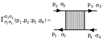
Figure 2: Diagrammatic representation of the four-point vertex with spin indices $\sigma_{1}$, $\sigma_{2}$, $\sigma_{3}$, and $\sigma_{4}$, which is irreducible with respect to particle-hole pairs.

In the limit of $q\rightarrow 0$, the Ward identity (42) is reduced to the following relation,

$$\hat{\mathcal{T}}^{\nu}(p,p)=i\alpha(\mbox{\boldmath$\mathcal{L}$}(p)\times\mbox{\boldmath$\sigma$})\cdot\mbox{\boldmath$n$}_{\nu}.$$ (47)

The above relation is not so trivial. Thus it is worth while examining (47) in more details. Substituting Eq.(47) into Eq.(43) with $q=0$, and using the following identity, which is derived from (26),

$$\hat{G}(p)i\alpha(\mbox{\boldmath$\mathcal{L}(p)$}\times\mbox{\boldmath$\sigma$})_{z}\hat{G}(p)=\left(\begin{array}[]{cc}0&G_{\uparrow\downarrow}(p)\\ -G_{\downarrow\uparrow}(p)&0\end{array}\right),$$ (50)

we find that the identity (47) with $\nu=z$ is equivalent to the following relations for the self-energy functions,

$$\Sigma_{\uparrow\downarrow}(p) = \sum_{p^{\prime}}[\Gamma_{\uparrow\downarrow}^{\downarrow\uparrow}(p,p;p^{\prime},p^{\prime})G_{\uparrow\downarrow}(p^{\prime})$$ (51)

$$-\Gamma_{\uparrow\downarrow}^{\uparrow\downarrow}(p,p;p^{\prime},p^{\prime})G_{\downarrow\uparrow}(p^{\prime})],$$

$$\Sigma_{\downarrow\uparrow}(p) = \sum_{p^{\prime}}[\Gamma_{\downarrow\uparrow}^{\uparrow\downarrow}(p,p;p^{\prime},p^{\prime})G_{\downarrow\uparrow}(p^{\prime})$$ (52)

$$- \Gamma_{\downarrow\uparrow}^{\downarrow\uparrow}(p,p;p^{\prime},p^{\prime})G_{\uparrow\downarrow}(p^{\prime})],$$

$$\sum_{p^{\prime}}\Gamma_{\uparrow\uparrow}^{\downarrow\uparrow}(p,p;p^{\prime},p^{\prime})G_{\uparrow\downarrow}(p^{\prime})=\sum_{p^{\prime}}\Gamma_{\uparrow\uparrow}^{\uparrow\downarrow}(p,p;p^{\prime},p^{\prime})G_{\downarrow\uparrow}(p^{\prime}),$$ (53)

$$\sum_{p^{\prime}}\Gamma_{\downarrow\downarrow}^{\downarrow\uparrow}(p,p;p^{\prime},p^{\prime})G_{\uparrow\downarrow}(p^{\prime})=\sum_{p^{\prime}}\Gamma_{\downarrow\downarrow}^{\uparrow\downarrow}(p,p;p^{\prime},p^{\prime})G_{\downarrow\uparrow}(p^{\prime}).$$ (54)

Here $\Gamma_{\sigma_{1}\sigma_{2}}^{\sigma_{3}\sigma_{4}}$ is four-point vertex functions $\hat{\Gamma}$ which appear in eq.(43). The interpretation of the identity relations (51)-(54) in terms of the diagrammatic language is as follows. In FIG.3, we depict diagrams which represent the off-diagonal self-energy $\Sigma_{\uparrow\downarrow}$. It is noted that the four-point vertex functions $\hat{\Gamma}$ in FIG.3 are obtained by rotating the four-point vertex shown in FIG.2 by 90 ^∘. Thus, the four-point vertex functions in FIG.3 are not irreducible with respect to particle-hole pairs in the horizontal direction. Among these diagrams, FIGs.3(a) and 3(b) are also expressed in the form of FIG.3(c), since in the four-point vertex in FIGs.3(a) and 3(b), there should be at least one $G_{\uparrow\downarrow}$-line. We note that the way of expressing $\Sigma_{\uparrow\downarrow}$ in the form of FIG.3(c) is not unique. The double counting occurs for diagrams which are also rewritten in the form of FIG.3(d), because the four point vertex in FIG.3(d) contains two more $G_{\uparrow\downarrow}$-lines than that in FIG.3(c), and thus the diagrams of the form FIG.3(d) are expressed in the form of FIG.3(c) in two different ways. We show in FIG.4 some examples of this double counting which occurs for $\sum_{p^{\prime}}\Gamma_{\uparrow\downarrow}^{\downarrow\uparrow}(p,p;p^{\prime},p^{\prime})G_{\uparrow\downarrow}(p^{\prime})$ etc. In FIGs.4(a), (b), and (c), we depict some examples of the second-order diagrams for $\hat{\mathcal{T}}^{\nu}(p+q/2,p-q/2)$. The Ward identity relates these three different diagrams, respectively, to the diagrams FIGs.4(d), (e), and (f), which express the second-order terms of $\Sigma_{\uparrow\downarrow}$. The diagrams FIGs.4(d) and (e) are parts of the diagram FIG.3(c), and the diagrams FIG.4(f) is a part of the diagram FIG.3(d). Apparently, these three self-energy diagrams FIGs.4(d), (c), and (f) are equivalent to each other, and double counting of diagrams occurs in FIG.3(c). Thus, $\Sigma_{\uparrow\downarrow}$ is represented by FIG.3(c) from which the duplicate diagrams of the form FIG.3(d) are subtracted. This amounts to the identity (51). We can also give a similar interpretation to Eq.(52). The implication of Eqs.(53) and (54) is more transparent. The left- and right-hand sides of Eq.(53) are nothing but two equivalent representations of $\Sigma_{\uparrow\uparrow}$. In FIG.4, we exhibit some examples of this equivalence. FIGs.4(g) and (h) are examples of diagrams for $\hat{\mathcal{T}}^{\nu}(p+q/2,p=q/2)$, which are, respectively, related to the self-energy diagrams FIGs.4(i) and (j), which constitute $\Sigma_{\uparrow\uparrow}$. These equivalent self-energy diagrams are, respectively, a part of $\sum_{p^{\prime}}\Gamma_{\uparrow\uparrow}^{\downarrow\uparrow}(p,p;p^{\prime},p^{\prime})G_{\uparrow\downarrow}(p^{\prime})$ and a part of $\sum_{p^{\prime}}\Gamma_{\uparrow\uparrow}^{\uparrow\downarrow}(p,p;p^{\prime},p^{\prime})G_{\downarrow\uparrow}(p^{\prime})$. This amounts to the relation (53). The relation holds for any higher-order diagrams. Eq.(54) also expresses $\Sigma_{\downarrow\downarrow}$ in two different manners.

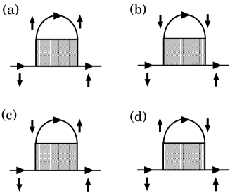
Figure 3: Diagrams representing the off-diagonal self-energy $\Sigma_{\uparrow\downarrow}$. The gray box is a four point vertex. The up and down arrows, respectively, express the up and down spins.

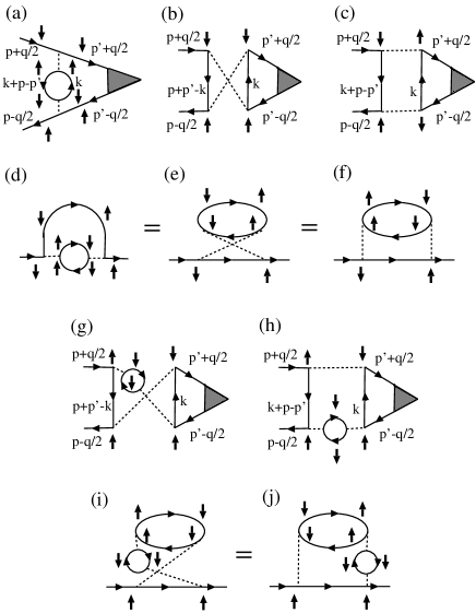
Figure 4: (a), (b), (c) Examples of second order diagrams which constitute $\hat{\mathcal{T}}^{\nu}(p+q/2,p-q/2)$. Broken lines represent the Coulomb interaction $U$. Black triangle represents the bare vertex $\hat{\mathcal{T}}_{0}^{\nu}$. (d), (e) Second-order self-energy diagrams which constitute $\sum_{p^{\prime}}\Gamma_{\uparrow\downarrow}^{\downarrow\uparrow}(p,p;p^{\prime},p^{\prime})G_{\uparrow\downarrow}(p^{\prime})$. The diagrams (d) and (e) are, respectively, related to the diagrams (a) and (b) via the Ward identity. (f) A second-order self-energy diagrams which constitute $\sum_{p^{\prime}}\Gamma_{\uparrow\downarrow}^{\uparrow\downarrow}(p,p;p^{\prime},p^{\prime})G_{\downarrow\uparrow}(p^{\prime})$. The diagram (f) is related to the diagram (c) via the Ward identity. Note that the self-energy diagrams (d), (e), and (f) are equivalent to each other. (g), (h) Examples of third-order diagrams for $\hat{\mathcal{T}}^{\nu}(p+q/2,p-q/2)$. (i) A third-order self-energy diagram which constitute $\sum_{p^{\prime}}\Gamma_{\uparrow\uparrow}^{\uparrow\downarrow}(p,p;p^{\prime},p^{\prime})G_{\downarrow\uparrow}(p^{\prime})$. The diagram (i) is related to the diagram (g) via the Ward identity. (j) A third-order diagram which constitute $\sum_{p^{\prime}}\Gamma_{\uparrow\uparrow}^{\downarrow\uparrow}(p,p;p^{\prime},p^{\prime})G_{\uparrow\downarrow}(p^{\prime})$. The diagram (j) is related to the diagram (h) via the Ward identity. Note that the diagram (i) is equivalent to the diagram (j).

II.3 Magnetism: Pauli and van-Vleck-like spin susceptibilities

As mentioned in the introduction, one of the unique magnetic properties in inversion-symmetry-broken systems is the existence of a van-Vleck-like spin susceptibility which stems from magnetic response of electrons occupying the momentum space sandwiched between spin-orbit splitted two Fermi surfaces. In this section we obtain general formulae for the Pauli and van-Vleck-like spin susceptibilities taking into account electron correlation effects in a formally exact way. The uniform spin susceptibility is easily obtained from (26) and (27) by using

$$\chi_{\mu\mu}=-\frac{d}{dH_{\mu}}T\sum_{\varepsilon_{n}}\sum_{k}\mu_{\rm B}{\rm tr}[\sigma_{\mu}\hat{G}(p)]|_{H_{\mu}\rightarrow 0}.$$ (55)

In the case of cubic systems, a straightforward calculation gives,

$$\chi_{zz} = \mu_{\rm B}^{2}\sum_{\tau=\pm}\sum_{k}\frac{z_{k\tau}}{4T\cosh^{2}(\frac{\varepsilon^{*}_{k\tau}}{2T})}\Lambda_{\rm P}^{\rm cub}(\varepsilon_{k\tau}^{*},\mbox{\boldmath$k$})$$ (56)

$$+ \mu_{\rm B}^{2}\sum_{\tau=\pm}\sum_{k}\frac{-\tau f(\varepsilon^{*}_{k\tau})}{\alpha|{\rm Re}~{}\mbox{\boldmath$\mathcal{L}$}(\varepsilon_{k\tau}^{*},\mbox{\boldmath$k$})|}\Lambda^{\rm cub}_{\rm V}(\varepsilon_{k\tau}^{*},\mbox{\boldmath$k$}),$$

with $f(\varepsilon)$ the Fermi distribution function. Here the three-point vertex functions $\Lambda^{\rm cub}_{\rm P}$ and $\Lambda^{\rm cub}_{\rm V}$ are,

$$\Lambda^{\rm cub}_{\rm P}(p) = \hat{\mathcal{L}}_{0z}^{2}(1-\frac{1}{\mu_{\rm B}}\frac{\partial\Sigma_{0}(p)}{\partial H_{z}})$$ (57)

$$- \frac{\hat{\mathcal{L}}_{0z}\hat{\mathcal{L}}_{x}}{\mu_{\rm B}}\frac{\partial\Sigma_{x}(p)}{\partial H_{z}}-\frac{\hat{\mathcal{L}}_{0z}\hat{\mathcal{L}}_{y}}{\mu_{\rm B}}\frac{\partial\Sigma_{y}(p)}{\partial H_{z}},$$

$$\Lambda^{\rm cub}_{\rm V}(p) = (\hat{\mathcal{L}}_{x}^{2}+\hat{\mathcal{L}}_{y}^{2})(1-\frac{1}{\mu_{\rm B}}\frac{\partial\Sigma_{0}(p)}{\partial H_{z}})$$ (58)

$$+ \frac{\hat{\mathcal{L}}_{0z}\hat{\mathcal{L}}_{x}}{\mu_{\rm B}}\frac{\partial\Sigma_{x}(p)}{\partial H_{z}}+\frac{\hat{\mathcal{L}}_{0z}\hat{\mathcal{L}}_{y}}{\mu_{\rm B}}\frac{\partial\Sigma_{y}(p)}{\partial H_{z}}.$$

The first and second terms of (56) are, respectively, the Pauli and van-Vleck-like terms. The van-Vleck-like term is not much affected by superconducting transition if the magnitude of the spin-orbit splitting $\alpha|\mbox{\boldmath$\mathcal{L}$}(p)|$ is sufficiently larger than the superconducting gap.

In the case of the tetragonal symmetry with a potential gradient along $\mbox{\boldmath$n$}=(0,0,1)$ (i.e. the Rashba interaction), $\mbox{\boldmath{$\mathcal{L}$}}_{0}(k)$ is parametrized as $\mbox{\boldmath$t$}_{0}(k)\times\mbox{\boldmath$n$}$. The vector $(t_{0x},t_{0y},0)$ transforms like $(k_{x},k_{y},0)$. Then, using a vector $\mbox{\boldmath$t$}(p)=\mbox{\boldmath$n$}\times\mbox{\boldmath{$\mathcal{L}$}}(p)$ and a unit vector $\hat{\mbox{\boldmath$t$}}(p)=\mbox{\boldmath$t$}(p)/|\mbox{\boldmath$t$}(p)|$, we express the spin susceptibility as,

$$\chi_{zz}=\mu_{\rm B}^{2}\sum_{\tau=\pm}\sum_{k}\frac{-\tau f(\varepsilon^{*}_{k\tau})}{\alpha|{\rm Re}~{}\mbox{\boldmath$t$}(\varepsilon_{k\tau}^{*},\mbox{\boldmath$k$})|}\Lambda^{sz}(\varepsilon_{k\tau}^{*},\mbox{\boldmath$k$}),$$ (59)

$$\chi_{xx}=\chi_{xx}^{\rm Pauli}+\chi_{xx}^{\rm VV},$$ (60)

$$\chi_{xx}^{\rm Pauli}=\mu_{\rm B}^{2}\sum_{\tau=\pm}\sum_{k}\frac{z_{k\tau}}{4T\cosh^{2}(\frac{\varepsilon^{*}_{k\tau}}{2T})}\hat{t}_{y}\Lambda_{\tau}^{sx}(\varepsilon_{k\tau}^{*},\mbox{\boldmath$k$}),$$ (61)

$$\chi_{xx}^{\rm VV}=\mu_{\rm B}^{2}\sum_{\tau=\pm}\sum_{k}\frac{-\tau f(\varepsilon^{*}_{k\tau})}{\alpha|{\rm Re}~{}\mbox{\boldmath$t$}(\varepsilon_{k\tau}^{*},\mbox{\boldmath$k$})|}\hat{t}_{x}\Lambda^{sx}_{+-}(\varepsilon_{k\tau}^{*},\mbox{\boldmath$k$}).$$ (62)

The three-point vertices $\Lambda^{sz}$, $\Lambda^{sx}_{+-}$, and $\Lambda^{sx}_{\tau}$ in the above expressions are given by

$$\Lambda^{sz}(p)=1-\frac{1}{\mu_{\rm B}}\frac{\partial\Sigma_{0}(p)}{\partial H_{z}},$$ (63)

$$\Lambda^{sx}_{\tau}(p)=\hat{t}_{y}(1-\frac{1}{\mu_{\rm B}}\frac{\partial\Sigma_{x}}{\partial H_{x}})+\frac{\hat{t}_{x}}{\mu_{\rm B}}\frac{\partial\Sigma_{y}}{\partial H_{x}}-\frac{\tau}{\mu_{\rm B}}\frac{\partial\Sigma_{0}}{\partial H_{x}},$$ (64)

$$\Lambda_{+-}^{sx}(p)=\hat{t}_{x}(1-\frac{1}{\mu_{\rm B}}\frac{\partial\Sigma_{x}}{\partial H_{x}})-\frac{\hat{t}_{y}}{\mu_{\rm B}}\frac{\partial\Sigma_{y}}{\partial H_{x}}.$$ (65)

As seen from (59) and (60), $\chi_{zz}$ is given only by the van-Vleck-like susceptibility, while $\chi_{xx}$ consists of both the Pauli and van-Vleck-like terms.

We note that in the limit of $\alpha\rightarrow 0$ (the inversion symmetry and the spin rotation symmetry are recovered),

$$\frac{\partial\Sigma_{x}}{\partial H_{x}}\rightarrow\frac{\partial\Sigma_{0}}{\partial H_{z}}.$$ (66)

This relation is easily verified by rotating the spin axes as $\sigma_{x}\rightarrow\sigma_{z}$, $\sigma_{z}\rightarrow-\sigma_{x}$, and $\sigma_{y}\rightarrow\sigma_{y}$, and noticing that this rotation transforms $(\Sigma_{\uparrow\downarrow}+\Sigma_{\downarrow\uparrow})/2$ into $(\Sigma_{\uparrow\uparrow}-\Sigma_{\downarrow\downarrow})/2$. Thus, Eqs.(59) and (60) leads $\chi_{zz}=\chi_{xx}$ in the limit of $\alpha\rightarrow 0$.

We see from (59) and (60) that both the Pauli term and the van-Vleck-like term are enhanced by the factors $\Lambda^{sz}$, $\Lambda^{sz}_{+-}$, and $\Lambda^{sz}_{\tau}$. If the density of states weakly depends on energy, and the spin-orbit splitting is much smaller than the Fermi energy, these three enhancement factors take values of the same order. However, when the energy dependence of the density of states is substantial, the enhancement of the van-Vleck-like susceptibility due to the electron correlation effect may be quite distinct from that of the Pauli term. We will consider such an example in Sec.III in connection with the heavy fermion superconductor CePt₃Si.

For experimental studies on superconducting states, it is important to discriminate between the Pauli susceptibility which decreases in the spin-singlet superconducting state, and the orbital susceptibility which is not affected by the superconducting transition. Usually, this discrimination is achieved by experimentally observing the temperature dependence of the spin susceptibility in the normal state, and identifying the temperature-independent part with the orbital term. However, this idea fails for noncentrosymmetric superconductors because of the existence of the van-Vleck-like susceptibility $\chi_{xx}^{\rm VV}$. When the spin-orbit splitting is much larger than the superconducting gap as in the case of CePt₃Si, CeRhSi₃, and CeIrSi₃, the van-Vleck-like term $\chi_{xx}^{\rm VV}$ is not much influenced by the superconducting transition and takes a finite value even at $T=0$, though it exhibits temperature dependence at high temperatures like the Pauli susceptibility.

Here we demonstrate to what extent $\chi_{xx}^{\rm VV}$ varies as a function of temperature by using a simple model. We consider a two-dimensional electron system on a square lattice with the energy momentum dispersion relation,

$$\varepsilon_{k}=-2(\cos k_{x}+\cos k_{y}),$$ (67)

and the Rashba spin-orbit interaction $\alpha(\mbox{\boldmath$t$}_{0}(k)\times\mbox{\boldmath$n$})\cdot\mbox{\boldmath$\sigma$}$. We put the hopping integral $t=1$ in (67). To preserve the periodicity of the energy band in the momentum space, we assume the form of $\mbox{\boldmath$t$}_{0}(k)$ as

$$\mbox{\boldmath$t$}_{0}(k)=(\sin\frac{k_{x}}{2},\sin\frac{k_{y}}{2},0).$$ (68)

This model can not be directly related with heavy fermion superconductors such as CePt₃Si, CeRhSi₃, etc. which have the complicated three-dimensional Fermi surfaces. Nevertheless, this simple model is quite instructive in that it demonstrates the strong temperature dependence of $\chi_{xx}^{\rm VV}$. For simplicity we neglect electron-electron interaction, and consider the half-filling case $n=1$, in which the van Hove singularity of the density of states gives rise to the temperature-dependence of the spin susceptibility. For $\alpha\neq 0$, to keep the electron density $n=1$, we need to add a counter term

$$-\delta\mu\sum_{k}c_{k}^{\dagger}c_{k},$$ (69)

with $\delta\mu=-\alpha^{2}/8$ to the Hamiltonian. The calculated results of $\chi_{xx}^{\rm Pauli}$ and $\chi_{xx}^{\rm VV}$ for some values of $\alpha$ are plotted as a function of temperature in FIG.5. It is seen that as $T$ increases, the curves of $\chi_{xx}^{\rm VV}$ and $\chi_{xx}^{\rm Pauli}$ approach to each other, and for $T\gg\alpha$, there is no substantial difference between them. The van-Vleck-like term $\chi_{xx}^{\rm VV}$ varies as a function of temperature, reflecting the singular energy dependence of the density of states in the model (67). If we take into account electron correlation effects, the energy dependence of the density of states is much enhanced, and thus, as $T$ is changed, $\chi_{xx}^{\rm VV}$ varies more drastically than the non-interacting case. This calculation suggests that it is almost impossible to distinguish the van-Vleck-like term from the Pauli susceptibility merely by analyzing experimental data of temperature dependence of the spin susceptibility in the normal state.

It is also worth while examining the anisotropy of the spin susceptibility due to the spin-orbit interaction. The calculated results of $\chi_{xx}$ and $\chi_{zz}$ as a function of $T$ are plotted in FIG.6 for several values of $\alpha$. It shows that the anisotropy becomes large for $T<\alpha|\mbox{\boldmath$t$}_{0k}|$. The magnitude of the anisotropy $|\chi_{xx}-\chi_{zz}|/\chi_{xx}$ is at most of order $\sim\alpha|\mbox{\boldmath$t$}_{0k}|/E_{F}$, as easily expected from (59) and (60). According to the LDA calculations for the heavy fermion superconductor CePt₃Si, the ratio $\alpha|\mbox{\boldmath$t$}_{0k}|/E_{F}$ is of order $\sim 0.1$.hari ; sam Although the de Haas van Alphen experiment for this system has not yet detected the spin-orbit splitted Fermi surfaces, the measurement for a related system LaPt₃Si support the existence of the spin-orbit splitting of which the magnitude is of this order.hari Thus, it is expected that the anisotropy of the spin susceptibility for CePt₃Si is at most $\sim 0.1$, which seems to be consistent with the experimental observation of the susceptibility.take ; met

Figure 5: $\chi_{xx}^{\rm Pauli}$ and $\chi_{xx}^{\rm VV}$ versus $T$. Each lines are, respectively, $\chi_{xx}^{\rm VV}$ for $\alpha=0.1$ (top solid line), $\chi_{xx}^{\rm Pauli}$ for $\alpha=0.1$ (top dotted line), $\chi_{xx}^{\rm VV}$ for $\alpha=0.5$ (bottom solid line), and $\chi_{xx}^{\rm Pauli}$ for $\alpha=0.5$ (bottom dotted line).

Figure 6: $\chi_{xx}$ and $\chi_{zz}$ versus $T$. Each lines are, respectively, $\chi_{zz}$ for $\alpha=0.1$ (top dotted line), $\chi_{xx}$ for $\alpha=0.1$ (top solid line), $\chi_{zz}$ for $\alpha=0.5$ (middle dotted line), $\chi_{xx}$ for $\alpha=0.5$ (middle solid line), $\chi_{zz}$ for $\alpha=1.0$ (bottom dotted line), and $\chi_{xx}$ for $\alpha=1.0$ (bottom solid line).

II.4 Transport coefficients

Generally, the absence of inversion symmetry brings about remarkable transport properties such as the anomalous Hall effect,kl ; jun the thermal anomalous Hall effect, the spin Hall effect,she ; she2 and magnetoelectric effects.lev ; ede0 In this section, we argue these phenomena with particular emphasis on the role of electron correlation effects. We mainly consider the case of the Rashba spin-orbit interaction with $\mbox{\boldmath$\mathcal{L}$}_{0}=\mbox{\boldmath$t$}_{0}\times\mbox{\boldmath$n$}$ in which the above-mentioned effects are more salient than the case of cubic systems with the Dresselhaus interaction.

II.4.1 Anomalous Hall effect

Here, we consider the anomalous Hall effect due to the Rashba spin-orbit interaction. The general theoretical description of the anomalous Hall effect due to the spin-orbit interaction was given by Karplus-Luttinger many years ago.kl The key ingredient of the Karplus-Luttinger-type anomalous Hall effect is the existence of a dissipationless transverse current which is induced by the paramagnetic Zeeman effect and stems from the anomalous velocity, $\nabla_{k}\alpha(\mbox{\boldmath$t$}_{0}(k)\times\mbox{\boldmath$n$})\cdot\mbox{\boldmath$\sigma$}$. In the case of the Rashba spin-orbit interaction, there is no $z$-component of the anomalous velocity, and thus this effect exists only for an applied magnetic field along the $z$-direction. In heavy fermion systems, the spin-orbit interaction caused by heavy atoms like Ce and U may also give rise to the anomalous Hall effect as experimentally observed in several systems such as CeRu₂Si₂, CeAl₃, and UPt₃.anh ; ahe1 ; ahe2 ; yam1 ; yam2 The strong anisotropic dependence on an external magnetic field of the Rashba-interaction-induced anomalous Hall effect makes a clear difference from the conventional anomalous Hall effect observed in the systems with inversion symmetry. Note that in the case of cubic systems with the Dresselhaus interaction, such a strong anisotropy does not exist.

The Hall conductivity for a magnetic field in the $z$-direction is defined as

$$\sigma_{xy}=\lim_{\omega\rightarrow 0}\frac{1}{i\omega}K_{xy}(i\omega_{n})|_{i\omega_{n}\rightarrow\omega+i0},$$ (70)

$$K_{xy}(i\omega_{n})=\int^{1/T}_{0}d\tau\langle T_{\tau}\{J_{x}(\tau)J_{y}(0)\}\rangle e^{i\omega_{n}\tau}.$$ (71)

The total charge current $J_{\mu}$ is,

$$J_{\mu}=e\sum_{k}c^{\dagger}_{k}\hat{v}_{k\mu}c_{k},$$ (72)

where the velocity $\hat{v}_{k\mu}$ is

$$\hat{v}_{k\mu}=\nabla_{k_{\mu}}(\varepsilon_{k}+\alpha\mbox{\boldmath$\sigma$}\cdot(\mbox{\boldmath$t$}_{0}(\mbox{\boldmath$k$})\times\mbox{\boldmath$n$})).$$ (73)

Since the anomalous Hall effect is caused by the interplay between the spin-orbit interaction and the Zeeman coupling with an external magnetic field, we neglect the orbital diamagnetic effect of the magnetic field which yields the normal Hall effect. Then the Hamiltonian under consideration is given by Eqs.(1) and (4) with $\mbox{\boldmath$H$}=(0,0,H_{z})$. From Eq.(34), the charge velocity vertex fully dressed by electron-electron interaction is given by,

$$\hat{\Lambda}^{c}_{\mu}(p,p) = \nabla_{k_{\mu}}(\varepsilon_{k}+\Sigma_{0}(p))+\nabla_{k_{\mu}}\Sigma_{z}(p)\sigma^{z}$$ (74)

$$+\alpha\nabla_{k_{\mu}}(t_{y}(p)\sigma^{x}-t_{x}(p)\sigma^{y}).$$

The last term of the right-hand side of (74) is the anomalous velocity. In the above expression of $\hat{\Lambda}^{c}_{\mu}$, the vertex corrections associated with dissipative processes which are important for the total momentum conservationyy are not included. The dissipative vertex corrections cannot be taken into account by the procedure presented above. However, their contributions to the anomalous Hall conductivity are negligible in the case that the spin-orbit-splitting is much larger than the quasiparticle damping because of the following reason. According to the general argument of the Fermi liquid theory for non-equilibrium transport coefficients, the dissipative vertex corrections are obtained by extracting the particle-hole pair $G^{R}G^{A}$ with $G^{R(A)}$ the retarded (advanced) single-particle Green function after the analytic continuation of $K_{xy}(i\omega_{n})$, since only $G^{R}G^{A}$ is singular in the limit of $\omega\rightarrow 0$ for infinitesimally small quasiparticle damping.eli In our case, as will be shown below, the particle-hole pair $G_{+}G_{+}$ and $G_{-}G_{-}$ do not enter into the expression of the anomalous Hall conductivity, and only the pair $G_{+}G_{-}$ contributes. When the spin-orbit-splitting is sufficiently larger than the quasiparticle damping, the particle-hole pairs $G_{+}^{R}G_{-}^{A}$ and $G_{+}^{R}G_{-}^{A}$ are not singular, and do not yield dissipative processes. Thus, we can ignore the dissipative vertex corrections for systems with large spin-orbit splitting. As a matter of fact, for the noncentrosymmetric heavy fermion superconductors CePt₃Si and CeRhSi₃, the typical size of the spin-orbit-splitting is of order $0.1E_{F}$ with $E_{F}$ the Fermi energy, and dominates over the quasiparticle damping.hari ; sam ; kim2 Then, the current-current correlation function $K_{xy}$ is expressed in terms of the Green functions,

$$K_{xy}(i\omega) = T\sum_{\varepsilon_{n}}\sum_{k}{\rm tr}[\hat{\Lambda}^{c}_{x}(p+q,p)\hat{G}(p+q)$$ (75)

$$\times\hat{v}_{ky}\hat{G}(p)].$$

Here $q=(i\omega,0,0,0)$. Collecting terms linear in $H_{z}$ for $H_{z}\rightarrow 0$, we find that only the anomalous velocity term in Eqs.(73) and (74) gives non-vanishing contributions to $K_{xy}(i\omega)$, which have the form $\sum_{p}f(\mbox{\boldmath$k$}){\rm tr}[\sigma^{x}\hat{G}(p)\sigma^{y}\hat{G}(p+q)]$ or $\sum_{p}f(\mbox{\boldmath$k$}){\rm tr}[\sigma^{y}\hat{G}(p)\sigma^{x}\hat{G}(p+q)]$, where $f(\mbox{\boldmath$k$})$ is the even function of momentum $k$. Using the assumption that the quasiparticle damping is much smaller than the spin-orbit-splitting, we obtain,

$$\frac{d}{dH_{z}}\sum_{p}f(\mbox{\boldmath$k$}){\rm tr}[\sigma^{y}\hat{G}(p)\sigma^{x}\hat{G}(p+q)]|_{H_{z}\rightarrow 0}=$$

$$i\sum_{p}[\frac{d}{dH_{z}}(\xi_{+}^{2}(p)\xi_{+}^{2}(p+q)-\xi_{-}^{2}(p)\xi_{-}^{2}(p+q))|_{H_{z}\rightarrow 0}$$

$$\times(G_{+}(p)G_{-}(p+q)-G_{-}(p)G_{+}(p+q))$$

$$+\frac{d}{dH_{z}}(\xi_{+}^{2}(p)\xi_{-}^{2}(p+q)-\xi_{-}^{2}(p)\xi_{+}^{2}(p+q))|_{H_{z}\rightarrow 0}$$

$$\times(G_{+}(p)G_{+}(p+q)-G_{-}(p)G_{-}(p+q))].$$ (76)

The last term of the right-hand side of (76) does not contribute to ${\rm Re}~{}\sigma_{xy}$. In the limit of $\omega\rightarrow 0$,

$$\frac{d}{dH_{z}}(\xi_{+}^{2}(p)\xi_{+}^{2}(p+q)-\xi_{-}^{2}(p)\xi_{-}^{2}(p+q))|_{H_{z}\rightarrow 0}$$

$$=-\frac{1}{\alpha|{\rm Re}~{}\mbox{\boldmath$t$}(p)|}(\mu_{\rm B}-\frac{\partial\Sigma_{0}(p)}{\partial H_{z}}).$$ (77)

Using (75), (76), and (77), we end up with,

$$\frac{{\rm Re}~{}\sigma_{xy}^{\rm AHE}}{H_{z}} = e^{2}\mu_{\rm B}\sum_{\tau=\pm}\sum_{k}\frac{-\tau f(\varepsilon^{*}_{k\tau})\Lambda^{sz}(\varepsilon_{k\tau}^{*},\mbox{\boldmath$k$})}{2\alpha|{\rm Re}~{}\mbox{\boldmath$t$}(\varepsilon_{k\tau}^{*},\mbox{\boldmath$k$})|^{3}}$$ (78)

$$\times(\partial_{k_{x}}t_{x\tau}\partial_{k_{y}}t_{0y}-\partial_{k_{x}}t_{y\tau}\partial_{k_{y}}t_{0x}).$$

Here $\partial_{k_{\mu}}t_{\nu\tau}\equiv\partial_{k_{\mu}}t_{\nu}(\varepsilon,\mbox{\boldmath$k$})|_{\varepsilon=\varepsilon_{k\tau}^{*}}$; i.e. $\partial_{k_{\mu}}$ does not operate on $\varepsilon_{k\tau}^{*}$ in the argument of $t_{\nu}(p)$. Since we have postulated that the spin-orbit splitting is much larger than the quasiparticle damping, the anomalous Hall conductivity $\sigma^{\rm AHE}_{xy}$ is not involved with any relaxation time, and thus determined only by dissipationless processes. It is noted that the anomalous Hall conductivity is enhanced by the factor $\Lambda^{sz}$ which is equivalent to the enhancement factor of $\chi_{zz}$, Eq.(59). In the heavy fermion system CePt₃Si, this enhancement factor is of order $\sim 60$, and the detection of the anomalous Hall effect is feasible in such strongly correlated electron systems. We would like to stress that in the expression of the anomalous Hall conductivity (78), not only electrons in the vicinity of the Fermi surface but also all electrons in the region of the Brillouin zone sandwiched between the spin-orbit-splitted two Fermi surfaces contribute, in accordance with the fact that $\chi_{zz}$ is dominated by the van-Vleck-like susceptibility.

II.4.2 Thermal anomalous Hall effect

We now consider the thermal anomalous Hall effect, which is the anomalous Hall effect for the heat current. To simplify the following analysis, we assume that the energy current due to the interaction between quasiparticles is negligible, and thus the heat current is mainly carried by nearly independent quasiparticles. We would like to discuss the validity of this assumption in the end of this section. Then, we can obtain the thermal anomalous Hall conductivity by using a method similar to that used in the previous section. Using the heat current related to the single-particle energy,

$$J_{Q\mu}=\sum_{k}c^{\dagger}_{k}\frac{1}{2}[\hat{v}_{k\mu}\hat{H}(p)+\hat{H(p)}\hat{v}_{k\mu}]c_{k},$$ (79)

we define the Hall conductivity for the heat current as,

$$\kappa_{xy}=\frac{1}{T}(L^{(2)}_{xy}-\sum_{\mu\nu}L^{(1)}_{x\mu}L^{(0)-1}_{\mu\nu}L^{(1)}_{\nu y}),$$ (80)

where $L^{(0)}_{\mu\nu}$ is equal to the conductivity tensor $\sigma_{\mu\nu}$, and,

$$L^{(m)}_{\mu\nu}=\lim_{\omega\rightarrow 0}\frac{1}{i\omega}K_{\mu\nu}^{(m)}(i\omega_{n})|_{i\omega\rightarrow\omega+i0},\quad m=1,2,$$ (81)

$$K_{\mu\nu}^{(1)}(i\omega_{n})=\int^{1/T}_{0}d\tau\langle T_{\tau}\{J_{Q\mu}(\tau)J_{\nu}(0)\}\rangle e^{i\omega_{n}\tau},$$ (82)

$$K^{(2)}_{\mu\nu}(i\omega_{n})=\int^{1/T}_{0}d\tau\langle T_{\tau}\{J_{Q\mu}(\tau)J_{Q\nu}(0)\}\rangle e^{i\omega_{n}\tau}.$$ (83)

Extending the argument in the previous subsection straightforwardly to the present case, we find that the anomalous Hall effect gives rise to the following terms to $L_{xy}^{(1)}$ and $L_{xy}^{(2)}$,

$$\frac{L_{xy}^{(m){\rm AHE}}}{H_{z}}=e^{2-m}\mu_{\rm B}\sum_{\tau=\pm}\sum_{k}(-\tau)(\varepsilon_{k\tau}^{*})^{m}f(\varepsilon^{*}_{k\tau})$$

$$\times\frac{\Lambda^{sz}(\varepsilon_{k\tau}^{*},\mbox{\boldmath$k$})}{2\alpha|{\rm Re}~{}\mbox{\boldmath$t$}(\varepsilon_{k\tau}^{*},\mbox{\boldmath$k$})|^{3}}(\partial_{k_{x}}t_{x\tau}\partial_{k_{y}}t_{0y}-\partial_{k_{x}}t_{y\tau}\partial_{k_{y}}t_{0x}),$$ (84)

with $m=1,2$. Then, the expression for the thermal anomalous Hall conductivity $\kappa_{xy}^{\rm AHE}$ is given by Eqs.(80) and (84). As in the case of the anomalous Hall effect for the charge current, the thermal anomalous Hall conductivity is also dominated by the contributions from electrons occupying the momentum space sandwiched between the spin-orbit-splitted Fermi surfaces. This property brings about a remarkable effect in superconducting states. In the superconducting state, when vortices are pinned in the mixed state, the Hall effect for the charge current does not exist. Instead, the thermal Hall effect for the heat current carried by the Bogoliubov quasiparticles is possible. Since we consider the magnetic field perpendicular to the $xy$-plane, electrons in the normal core do not contribute to the thermal transport in the direction parallel to the plane. Below the superconducting transition temperature $\sigma_{xy}$ is infinite while $L^{(1)}$ is finite. Thus the thermal Hall effect is governed by the first term of the right-hand side of (80), i.e. the coefficient $L_{xy}^{(2)}$. In contrast to the normal Hall effect for the heat current which decreases rapidly in the superconducting state, the coefficient $L_{xy}^{(2){\rm AHE}}$ is not affected by the superconducting transition when the magnitude of the spin-orbit-splitting is much larger than the superconducting gap as in the case of CePt₃Si and CeRhSi₃. Thus, even in the limit of $T\rightarrow 0$, $\kappa^{\rm AHE}_{xy}/(H_{z}T)$ takes a finite value. Moreover in heavy fermion systems, the magnitude of $\kappa^{\rm AHE}_{xy}/(H_{z}T)$ in the limit of $T\rightarrow 0$ is expected to be much enhanced by the factor $\Lambda^{sz}$.

Finally, we discuss the validity of the disregard for the heat current carried by the interaction between quasiparticles. In the vicinity of the Fermi surface, the quasiparticle approximation is applicable, and the interaction between quasiparticles is much reduced by the wave function renormalization factor $z^{2}_{k\tau}$, and may be negligible for heavy fermion systems. However, as seen from Eq.(84), the thermal anomalous Hall conductivity is dominated by the contributions away from the Fermi surface, which throws a doubt on this approximation. As a matter of fact, the above treatment of the heat current is justified as far as the spin-orbit splitting $\alpha|\mbox{\boldmath$t$}(0,\mbox{\boldmath$k$})|$ is much smaller than the Fermi energy $E_{F}$. For $\alpha|\mbox{\boldmath$t$}(0,\mbox{\boldmath$k$})|\ll E_{F}$, the quasiparticle approximation is still valid for all electrons in the region sandwiched between the spin-orbit splitted two Fermi surfaces. The relation $\alpha|\mbox{\boldmath$t$}(0,\mbox{\boldmath$k$})|\ll E_{F}$ holds when the carrier density is not so low. This condition is satisfied for any noncentrosymmetric heavy fermion superconductors CePt₃Si, CeRhSi₃, CeIrSi₃, and UIr.

II.4.3 Spin Hall effect

Recently, the existence of the spin Hall effect in the Rashba model has been extensively investigated by several authors.she ; she2 However, electron correlation effects on the spin Hall coefficient has not yet been fully elucidated. In this section, we explore the Fermi liquid theory for the spin Hall effect. The spin Hall effect is characterized by the transverse spin current induced by an electric field. For the Rashba model with the inversion symmetry breaking along the $z$-axis, the in-plane spin current with the magnetization in the $z$-direction is considered. Then, the spin Hall conductivity is defined as,

$$\sigma^{\rm SHE}_{xy}=\lim_{\omega\rightarrow 0}\frac{1}{i\omega}K^{\rm SHE}(i\omega_{n})|_{i\omega_{n}\rightarrow\omega+i0},$$ (85)

$$K^{\rm SHE}(i\omega_{n})=\int^{1/T}_{0}d\tau\langle T_{\tau}\{J^{sz}_{x}(\tau)J_{y}(0)\}\rangle e^{i\omega_{n}\tau}.$$ (86)

Here the total spin current $J^{sz}_{x}$ is,

$$J^{sz}_{x}=\frac{\mu_{\rm B}}{2}\sum_{k}c^{\dagger}_{k}(\hat{v}_{kx}\sigma^{z}+\sigma^{z}\hat{v}_{kx})c_{k}.$$ (87)

Note that we put the $g$ factor equal to 2. The spin current vertex function fully-dressed by electron-electron interaction is readily obtained from the Ward identity (42) which is, in the case of the Rashba interaction, rewritten as,

$$\sum_{\mu=0,x,y,z}q_{\mu}\hat{\Lambda}^{sz}_{\mu}(p+\frac{q}{2},p-\frac{q}{2})=$$

$$(-i\omega+\varepsilon_{k+\frac{q}{2}}+\Sigma_{0}(p+\frac{q}{2})-\varepsilon_{k-\frac{q}{2}}-\Sigma_{0}(p-\frac{q}{2}))\frac{\sigma^{z}}{2}$$

$$-\frac{i\alpha}{2}\mbox{\boldmath$\sigma$}\cdot[\mbox{\boldmath$t$}(p+\frac{q}{2})+\mbox{\boldmath$t$}(p-\frac{q}{2})]+\hat{\mathcal{T}}^{z}(p+\frac{q}{2},p-\frac{q}{2}).$$ (88)

We note that for $\omega/\mbox{\boldmath$q$}\rightarrow 0$ and small $q$, $\hat{\mathcal{T}}^{\nu}(p+q/2,p-q/2)$ is expanded as,

$$\hat{\mathcal{T}}^{\nu}(p+\frac{q}{2},p-\frac{q}{2})=\hat{\mathcal{T}}^{\nu}(p,p)+O(q^{2}).$$ (89)

The absence of the $q$-linear term in (89) is verified as follows. For $\omega=0$, in the Feynman diagrams which constitute $\hat{\mathcal{T}}^{z}(p+q/2,p-q/2)$, the total number of $G$-lines which depend on $q/2$ is equal to that of $G$-lines which depend on $-q/2$. Each diagram which is derived by differentiating a $G(p^{\prime}+q/2)$-line with respect to $q$ gives the same contribution as that obtained from the differentiation of $G(p^{\prime\prime}-q/2)$-line with respect to $-\mbox{\boldmath$q$}$ in the limit of $q\rightarrow 0$. This situation is diagrammatically depicted in FIG.7. Thus, all terms of order $O(q)$ in $q\cdot\nabla_{q}\hat{\mathcal{T}}^{z}(p+q/2,p-q/2)$ cancel with each other, which leads Eq.(89). Then, putting $\omega=0$ first and then taking the limit of $\mbox{\boldmath$q$}\rightarrow 0$ in (88), we have

$$\Lambda^{sz}_{\mu}(p,p)=\mu_{\rm B}\frac{\partial}{\partial k_{\mu}}(\varepsilon_{k}+\Sigma_{0}(p))\sigma^{z}.$$ (90)

We note that in the expression of $\Lambda^{sz}_{\mu}$, the vertex corrections associated with dissipative processes are not included, as in the case of the anomalous Hall effect considered in Sec.II.D.1. As long as the spin-orbit splitting is much larger than the quasiparticle damping, such vertex corrections are not important.

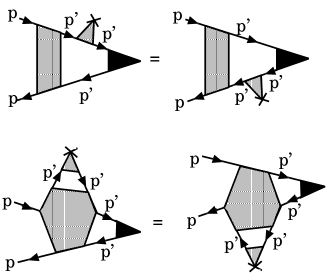
Figure 7: Diagrams representing $\lim_{q\rightarrow 0}\nabla_{q}\hat{\mathcal{T}}^{\nu}(p+q/2,p-q/2)$. The gray quadrangle is the four-point vertex irreducible with respect to particle-hole pairs. The black triangle represents $\hat{\mathcal{T}}^{\nu}$. The gray triangle with a cross is a three-point vertex generated by $q$-derivative. The gray hexagon is a six-point vertex irreducible with respect to particle-hole pairs.

By using (73) and (90), $K^{\rm SHE}(i\omega_{n})$ is recast into,

$$\sum_{p}{\rm tr}[\hat{\Lambda}^{sz}_{x}(p+q,p)\hat{G}(p)\hat{v}_{ky}\hat{G}(p+q)].$$ (91)

A straightforward calculation leads,

$$\sigma^{\rm SHE}_{xy}=e\mu_{\rm B}\sum_{k}\sum_{\tau=\pm}\frac{-\tau f(\varepsilon_{k\tau}^{*})\hat{t}_{x}(\varepsilon_{k\tau}^{*},\mbox{\boldmath$k$})\tilde{v}_{x\tau}\partial_{k_{y}}t_{0y}}{2\alpha|{\rm Re}~{}\mbox{\boldmath$t$}(\varepsilon_{k\tau}^{*},\mbox{\boldmath$k$})|^{2}},$$ (92)

where

$$\tilde{v}_{\mu\tau}=\partial_{k_{\mu}}(\varepsilon_{k}+\Sigma_{0}^{R}(\varepsilon,\mbox{\boldmath$k$}))|_{\varepsilon=\varepsilon_{k\tau}^{*}}.$$ (93)

In the expression of the spin Hall conductivity (92), the factors $\tilde{v}_{x\tau}$ and $\mbox{\boldmath$t$}(p)$ are not substantially affected by electron correlation effects, because the main effect of the electron correlation on these factors appears only through the deformation of the Fermi surface. Thus, the spin Hall conductivity $\sigma_{xy}^{\rm SHE}$ is not renormalized by electron correlation effects, but determined solely by the band structure.

II.4.4 Magnetoelectric effect

The existence of the spin-orbit interaction of the form $(\mbox{\boldmath t}_{0k}\times\nabla V)\cdot\mbox{\boldmath$\sigma$}$ gives rise to nontrivial coupling between charge and spin degrees of freedom, which results in interesting magnetoelectric effects. For example, there exists the bulk magnetization induced by the charge current flow, as pointed out by Levitov et al. many years ago.lev To argue this phenomenon, we consider the Rashba-type system with $\nabla V$ along the $z$-axis. The magnetization along the $x$-direction is generated by an electric field applied in the $y$-direction,

$$M_{x}=\Upsilon_{xy}E_{y}.$$ (94)

The inverse effect is also possible; i.e. an AC-magnetic field can yield the charge current flow,

$$J_{x}=-2\Upsilon_{xy}\frac{\partial B_{y}}{\partial t}.$$ (95)

The prefactor $2$ in (95) is due to the fact that in addition to the current directly induced by $\dot{B}$, there is a magnetization current $c(\nabla\times M)$. It is noted that analogous effects in the superconducting state, i.e. the supercurrent flow induced by the Zeeman magnetic field, and its inverse effect, are also argued by Edelstein, Yip, and the present author.ede1 ; ede2 ; yip ; fuji2

The formula of the magnetoelectric coefficient $\Upsilon_{xy}$ in the case without electron-electron interaction was obtained by Levitov et al.lev ; ede0 Here we consider effects of electron correlation on $\Upsilon_{xy}$, which may be important in the application to heavy fermion superconductors. In the normal state, the magnetoelectric coefficient $\Upsilon_{xy}$ is a non-equilibrium transport coefficient, to which the Fermi liquid corrections are obtained by the method developed by Eliashberg for the calculation of the electric conductivity.eli

According to the Kubo formula, the magnetoelectric coefficient is given by,

$$\Upsilon_{xy}(\omega)=\frac{1}{i\omega}K_{xy}^{\rm ME}(i\omega_{n})|_{i\omega_{n}\rightarrow\omega+i0},$$ (96)

$$K_{xy}^{\rm ME}(i\omega_{n})=\int^{1/T}_{0}d\tau\langle T_{\tau}\{S^{x}(\tau)J_{y}(0)\}\rangle e^{i\omega_{n}\tau}.$$ (97)

Applying the Eliashberg’s method,eli we can express this correlation function in terms of the Green functions and the three-point vertex functions for the spin density and the charge current density. The spin density vertex function required for the calculation of (97) is obtained from the Ward identity (42). Taking the limit of $\mbox{\boldmath$q$}\rightarrow 0$ of the Ward identity (42), we have the equation satisfied by the fully-dressed three-point vertex function of the spin density,

$$i\omega\hat{\Lambda}^{s\nu}_{0}(p+\frac{q}{2},p-\frac{q}{2})=\frac{\sigma_{\nu}}{2}[i\omega-\Sigma_{0}(p+\frac{q}{2})+\Sigma_{0}(p-\frac{q}{2})]$$

$$-\frac{\alpha}{2}[\mathcal{L}_{\nu}(p+\frac{q}{2})-\mathcal{L}_{\nu}(p-\frac{q}{2})]$$

$$+\frac{i\alpha}{2}(\{\mbox{\boldmath$\mathcal{L}$}(p+\frac{q}{2})+\mbox{\boldmath$\mathcal{L}$}(p-\frac{q}{2})\}\times\mbox{\boldmath$\sigma$})\cdot\mbox{\boldmath$n$}_{\nu}$$

$$-\hat{\mathcal{T}}^{\nu}(p+\frac{q}{2},p-\frac{q}{2}).$$ (98)

In the above expression, $q=(i\omega,\mbox{\boldmath$0$})$. Using Eq.(47), we extract $\omega$-linear terms of the right-hand side of (98) and take the limit $\omega\rightarrow 0$ arriving at,

$$\hat{\Lambda}^{s\nu}_{0}(p,p)=\frac{\sigma_{\nu}}{2}\left(1-\frac{\partial\Sigma_{0}(p)}{\partial(i\varepsilon_{n})}\right)-\frac{\alpha}{2}\frac{\partial\mathcal{L}_{\nu}(p)}{\partial(i\varepsilon_{n})}$$

$$-\frac{\partial\hat{\mathcal{T}}^{\nu}(p+q/2,p-q/2)}{\partial(i\omega)}\biggr{|}_{i\omega\rightarrow 0}.$$ (99)

Then, using Eqs.(99) and (74) for the spin density and charge velocity vertex functions, respectively, and extracting the factor $G^{R}_{\tau}(p)G^{A}_{\tau}(p)=2\pi iz_{k\tau}^{2}\delta(\varepsilon-\varepsilon_{k\tau}^{*})/(\omega+2i\gamma_{k\tau})$ after the analytical continuation to the real frequency, we have for small $\omega$,

$$\Upsilon_{xy}(\omega)=e\mu_{\rm B}\sum_{k}\sum_{\tau=\pm}\frac{\tau z_{k\tau}^{2}\Pi_{k\tau}}{4T\cosh^{2}(\frac{\varepsilon_{k\tau}^{*}}{2T})}\frac{i}{\omega+2i\gamma_{k\tau}},$$ (100)

$$\Pi_{k\tau} = \biggl{(}1-\frac{\partial\Sigma_{0}^{R}(\varepsilon_{k\tau}^{*},\mbox{\boldmath$k$})}{\partial\varepsilon}-\frac{\partial(\mathcal{T}^{x}_{\uparrow\downarrow}+\mathcal{T}^{x}_{\downarrow\uparrow})}{2\partial\omega}\biggr{|}_{\omega\rightarrow 0}\biggr{)}\mathcal{J}_{y\tau}$$ (101)

$$- \tau\biggl{(}\frac{\partial\Sigma_{x}(\varepsilon_{k\tau}^{*},\mbox{\boldmath$k$})}{\partial\varepsilon}+\frac{\partial(\mathcal{T}^{x}_{\uparrow\uparrow}+\mathcal{T}^{x}_{\downarrow\downarrow})}{2\partial\omega}\biggr{|}_{\omega\rightarrow 0}\biggr{)}\mathcal{I}_{y\tau},$$

with,

$$\mathcal{J}_{y\tau}=\hat{t}_{y}\tilde{v}_{y\tau}+\tau\alpha\partial_{k_{y}}t_{y\tau}+\Delta\mathcal{J},$$ (102)

$$\mathcal{I}_{y\tau}=\tilde{v}_{y\tau}+\tau(\partial_{k_{y}}t_{y\tau}\hat{t}_{y}+\partial_{k_{y}}t_{x\tau}\hat{t}_{x})+\Delta\mathcal{I}.$$ (103)

Here $\Delta\mathcal{J}$ and $\Delta\mathcal{I}$ are the contributions from the vertex corrections to the charge current which are required for preserving the momentum conservation law, and related to the quasiparticle damping $\gamma_{k\tau}$ by the Ward identity for the charge degrees of freedom.yy In the following we are not concerned with the explicit form of these vertex corrections, but merely assume that umklapp processes or impurity scattering break the momentum conservation, leading to a finite value of the dissipative transport coefficient.

In the expression of Eq.(100), the mass renormalization factor $z_{k\tau}$ cancels after carrying out the momentum sum $\sum_{k}$ in the DC limit $\omega\rightarrow 0$, and thus electron correlation effects appear only through $\Pi_{k\tau}$ and the factor $\gamma_{k\tau}/z_{k\tau}={\rm Im}\Sigma_{0}(\mbox{\boldmath$k$},\varepsilon_{k\tau}^{*})$. This factor is related to the resistivity $\rho\sim{\rm Im}\Sigma_{0}\sim c_{0}+AT^{2}$, where the constant $c_{0}$ is a residual resistivity due to impurity scattering. In heavy fermion systems, the coefficient of the $T$-square term of the resistivity $A$ is almost proportional to the square of the specific heat coefficient $\gamma^{2}$, which are much enhanced by electron correlation. The factor $\Pi_{k\tau}$ (101) is enhanced like the specific heat coefficient $\gamma$ because of the term proportional to $-\partial\Sigma_{0}^{R}(p)/\partial\varepsilon$. The other terms in $\Pi_{k\tau}$ are smaller than this term by a factor $\alpha|\mbox{\boldmath$t$}(p)|/E_{F}\ll 1$. Thus,

$$\Upsilon_{xy}\sim\frac{\gamma}{c_{0}+{\rm const.}\gamma^{2}T^{2}},$$ (104)

at low temperatures. In the temperature region where the resistivity exhibits $T^{2}$-dependence, $\Upsilon_{xy}$ behaves like $\sim 1/(\gamma T^{2})$, while in the zero temperature limit $\Upsilon_{xy}$ is enhanced by the factor $\gamma$.

III Superconducting state

III.1 Basic equations

The Fermi liquid theory in the normal state developed in the previous section can be straightforwardly extended to the superconducting state as in the case with inversion symmetry.leg ; mig ; fuji This task for the case of the Rashba interaction was done by the author in ref.fuji2 . Here we present the formalism for general forms of the spin-orbit interaction $\alpha\mbox{\boldmath$\mathcal{L}$}_{0}(k)\cdot\mbox{\boldmath$\sigma$}$. We add a pairing interaction to the model Hamiltonian (1), which may be originated from higher order interaction processes caused by the on-site Coulomb term $U$, or any other interactions.

In the conventional Nambu representation,sch the inverse of the single-particle Green’s function is defined as,

$$\hat{\mathcal{G}}^{-1}(p)=$$

$$\left(\begin{array}[]{cc}i\varepsilon_{n}-\hat{H}(p)+\mu_{\rm B}\mbox{\boldmath$\sigma$}\cdot\mbox{\boldmath$H$}&-\hat{\Delta}(p)\\ -\hat{\Delta}^{\dagger}(p)&i\varepsilon_{n}+\hat{H}^{t}(-p)-\mu_{\rm B}\mbox{\boldmath$\sigma$}^{t}\cdot\mbox{\boldmath$H$}\end{array}\right).$$ (107)

Here $\hat{H}(p)$ is given by the same expression as Eq.(6). However, the self-energy $\hat{\Sigma}(p)$ in this case includes both the normal Green function $\hat{G}(p)$ and the anomalous Green function $\hat{F}(p)$ presented below as internal lines.

$i\varepsilon_{n}-\hat{H}(p)+\mu_{\rm B}\mbox{\boldmath$\sigma$}\cdot\mbox{\boldmath$H$}$ and $i\varepsilon_{n}+\hat{H}^{t}(-p)-\mu_{\rm B}\mbox{\boldmath$\sigma$}^{t}\cdot\mbox{\boldmath$H$}$ in $\hat{\mathcal{G}}^{-1}(p)$ are diagonalized by the transformation $\hat{\mathcal{A}}(p)\hat{\mathcal{G}}^{-1}(p)\hat{\mathcal{A}}_{+}(p)$ with,

$$\hat{\mathcal{A}}(p)=\left(\begin{array}[]{cc}\hat{U}(p)&0\\ 0&\hat{U}^{t}_{+}(-p)\end{array}\right),$$ (110)

$$\hat{\mathcal{A}}_{+}(p)=\left(\begin{array}[]{cc}\hat{U}_{+}(p)&0\\ 0&\hat{U}^{t}(-p)\end{array}\right),$$ (113)

Here $\hat{U}(p)$ and $\hat{U}_{+}(p)$ have the same forms as in the normal state given by (15) and (18), respectively.

To diagonalize the superconducting gap $\hat{\Delta}(p)$, we need the assumption that ${\rm Im}\Sigma_{x}$ and ${\rm Im}\Sigma_{y}$ (and thus ${\rm Im}\mathcal{L}_{x,y}$) are negligible, which implies $\hat{U}_{+}(p)=\hat{U}^{\dagger}(p)$, and is justified in the absence of magnetic fields, i.e. $\mbox{\boldmath$H$}=0$. Under this condition, $\hat{\Delta}(p)$ and $\hat{\Delta}^{\dagger}(p)$ in $\hat{\mathcal{G}}^{-1}(p)$ are diagonalized by the transformation $\hat{\mathcal{A}}\hat{\mathcal{G}}^{-1}(p)\hat{\mathcal{A}}_{+}$ if and only if the gap function has the form,

$$\hat{\Delta}(p)=\Delta_{s}(k)i\sigma_{y}+\Delta_{t}(k)\mbox{\boldmath$\mathcal{L}$}(p)\cdot\mbox{\boldmath$\sigma$}i\sigma_{y}.$$ (114)

Eq.(114) implies that there is no Cooper pair between electrons on different Fermi surfaces $\varepsilon_{k+}$ and $\varepsilon_{k-}$, of which the existence gives rise to pair-breaking effects.

The inverse of Eq.(107) is readily obtained as,

$$\hat{\mathcal{G}}(p)=\left(\begin{array}[]{cc}\hat{G}(p)&\hat{F}(p)\\ \hat{F}^{\dagger}(p)&-\hat{G}^{t}(-p)\end{array}\right),$$ (117)

where

$$\hat{G}(p)=\sum_{\tau=\pm 1}\frac{1+\tau\hat{\mbox{\boldmath$\mathcal{L}$}}(p)\cdot\mbox{\boldmath$\sigma$}}{2}G_{\tau}(p),$$ (118)

$$\hat{F}(p)=\sum_{\tau=\pm 1}\frac{1+\tau\hat{\mbox{\boldmath$\mathcal{L}$}}(p)\cdot\mbox{\boldmath$\sigma$}}{2}i\sigma_{y}F_{\tau}(p),$$ (119)

and,

$$G_{\tau}(p)=\frac{\Xi_{\tau}^{(-)}(p)}{\Xi_{\tau}^{(+)}(p)\Xi_{\tau}^{(-)}(p)-\tilde{\Delta}_{k\tau}^{2}},$$ (120)

$$F_{\tau}(p)=\frac{\tilde{\Delta}_{k\tau}}{\Xi_{\tau}^{(+)}(p)\Xi_{\tau}^{(-)}(p)-\tilde{\Delta}_{k\tau}^{2}},$$ (121)

$$\Xi_{\tau}^{(\pm)}(p)=i\varepsilon\mp[\varepsilon_{k}-\mu+\Sigma_{0}(\pm p)+\tau\alpha|\mbox{\boldmath$\mathcal{L}$}(\pm p)|],$$ (122)

with $\tilde{\Delta}_{k\tau}=\Delta_{s}(k)+\tau|\mbox{\boldmath$\mathcal{L}$}(k)|\Delta_{t}(k)$. When the quasiparticle approximation is applicable,

$$G_{\tau}(p)=\frac{z_{k\tau}(i\varepsilon+\varepsilon_{k\tau}^{*})}{(i\varepsilon+i\gamma_{k\tau}{\rm sgn}\varepsilon)^{2}-E^{2}_{k\tau}},$$ (123)

$$F_{\tau}(p)=\frac{z_{k\tau}\Delta_{k\tau}}{(i\varepsilon+i\gamma_{k\tau}{\rm sgn}\varepsilon)^{2}-E^{2}_{k\tau}},$$ (124)

with $E_{k\tau}=\sqrt{\varepsilon_{k\tau}^{*2}+\Delta^{2}_{k\tau}}$ and $\Delta_{k\tau}=z_{k\tau}\tilde{\Delta}_{k\tau}$. The mass renormalization factor $z_{k\tau}$ is also given by the same expression as Eq.(31) with the self-energy $\hat{\Sigma}(p)$ replaced with that in the superconducting state.

Occasionally, some physical quantities for inversion-symmetry-broken systems are governed by electrons occupying the momentum space region between the spin-orbit splitted Fermi surfaces, as argued in the previous sections. In such cases, when the spin-orbit splitting is sufficiently large, the quasiparticle approximation cannot be generally justified, and it may be required to use the complicated expressions Eqs.(120) and (121). However, fortunately, for the noncentrosymmetric heavy fermion superconductors CePt₃Si and CeRhSi₃, the spin-orbit splitting is much larger than the superconducting gap, and thus any physical quantities governed by electrons occupying the momentum space region between the spin-orbit splitted Fermi surfaces are safely approximated by the quantities in the normal state, of which the calculation is much easier.

III.2 Paramagnetic properties

We now argue the paramagnetism of this system on the basis of the formalism presented above. The uniform spin susceptibility is calculated from the $\nu$-component of the magnetization

$$M_{\nu}=\frac{T}{2}\sum_{p}{\rm tr}\left[\left(\begin{array}[]{cc}\sigma_{\nu}&0\\ 0&-\sigma_{\nu}^{t}\\ \end{array}\right)\hat{\mathcal{G}}(p)\right].$$ (127)

In the derivation of the spin susceptibility, we ignore the magnetic-field-dependence of the superconducting gap, because the contributions from $\partial\Delta_{k\tau}/\partial H_{\nu}$ to the spin susceptibility is vanishingly small when the energy dependence of the density of states is nearly particle-hole symmetric.

In the case with cubic symmetry, the uniform spin susceptibility in the superconducting state is calculated as,

$$\chi_{zz}(T)=\mu_{\rm B}^{2}\sum_{\tau=\pm}\sum_{k}\frac{z_{k\tau}}{4T\cosh^{2}(\frac{E_{k\tau}}{2T})}\Lambda_{\rm P}^{\rm cub}(E_{k\tau},\mbox{\boldmath$k$})$$

$$-2\mu_{\rm B}^{2}T\sum_{\varepsilon_{n}}\sum_{k}[G_{+}(p)G_{-}(p)+F_{+}(p)F_{-}(p)]$$

$$\times\Lambda^{\rm cub}_{\rm V}(i\varepsilon_{n},\mbox{\boldmath$k$}).$$ (128)

The first and second terms of the right-hand side of (128) are, respectively, the Pauli and van-Vleck-like contributions. The three-point vertex functions $\Lambda^{\rm cub}_{\rm P}$ and $\Lambda^{\rm cub}_{\rm V}$ in Eq.(128) are slightly different from those appeared in the normal state (57) and (58) because the anomalous Green function $\hat{F}(p)$ also contributes to the self-energy $\hat{\Sigma}(p)$. However, as long as there is no strong spin fluctuation, the corrections to $\Lambda^{\rm cub}_{\rm P,V}$ due to the existence of the superconducting gap are small.leg In the case of $|\Delta_{k\tau}|\ll\alpha|\mbox{\boldmath$\mathcal{L}$}(p)|$, the quasiparticle approximation (123) and (124) is not applicable to the van-Vleck-like term. Thus, we will not write down its explicit form in Eq.(128). As a matter of fact, in this case, the van Vleck term is well approximated by the formula for the normal state (56). In the case of a spherical Fermi surface without electron-electron interaction, and $\mbox{\boldmath$\mathcal{L}$}_{0}(k)=(k_{x}(k_{y}^{2}-k_{z}^{2}),k_{y}(k_{z}^{2}-k_{x}^{2}),k_{z}(k_{x}^{2}-k_{y}^{2})$, if the condition $|\Delta_{k\tau}|\ll\alpha|\mbox{\boldmath$\mathcal{L}$}(p)|\ll E_{F}$ is satisfied, the spin susceptibility at zero temperature is $\chi_{zz}(0)\approx\frac{2}{3}\chi_{zz}(T_{c})$, since the van-Vleck-like term remains finite.

In the Rashba case, for a magnetic field perpendicular to the plane, the uniform spin susceptibility is given by,

$$\chi_{zz}(T) = -2\mu_{\rm B}^{2}T\sum_{\varepsilon_{n}}\sum_{k}[G_{+}(p)G_{-}(p)+F_{+}(p)F_{-}(p)]$$ (129)

$$\times\Lambda^{sz}(i\varepsilon_{n},\mbox{\boldmath$k$}).$$

For an in-plane magnetic field,fuji3

$$\chi_{xx}(T) = \mu_{\rm B}^{2}\sum_{\tau=\pm}\sum_{k}\frac{z_{k\tau}}{4T\cosh^{2}(\frac{E_{k\tau}}{2T})}\hat{t}_{y}\Lambda_{\tau}^{sx}(E_{k\tau},\mbox{\boldmath$k$})$$ (130)

$$- 2\mu_{\rm B}^{2}T\sum_{\varepsilon_{n}}\sum_{k}[G_{+}(p)G_{-}(p)+F_{+}(p)F_{-}(p)]$$

$$\times\hat{t}_{x}\Lambda^{sx}_{+-}(i\varepsilon_{n},\mbox{\boldmath$k$}).$$

Here we have ignored the corrections to the three-point vertex functions due to the superconducting gap again assuming that there is no strong ferromagnetic fluctuation. We are concerned with the case that the typical size of the spin-orbit splitting $2\alpha|\mbox{\boldmath$t$}(p)|$ is much larger than $|\Delta_{k}|$; i.e. the situation relevant to CePt₃Si and CeRhSi₃. In this case, the second term of the right-hand side of (130), which is the van-Vleck-like contribution, is approximated by the expression for the normal state $\chi_{xx}^{\rm VV}$ (62), and not affected by the superconducting transition, while the Pauli term, i.e. the first term of (130), vanishes at zero temperature. When the energy dependence of the density of states is sufficiently small, e.g. the case of the spherical Fermi surface $\varepsilon=k^{2}/(2m)$, we have $\chi_{xx}^{\rm SC}(T=0)/\chi_{xx}^{\rm SC}(T=T_{c})=1/2$, as pointed out by Edelstein, and Gorkov and Rashba.ede1 ; gor We would like to stress that the nonzero $\chi$ at zero temperature in the superconducting state is not due to the admixture of the spin singlet and triplet pairs, but rather attributed to the existence of the van-Vleck-like term caused by the spin-orbit interaction.

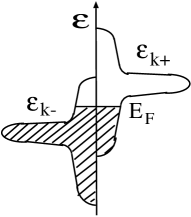
Figure 8: A schematic figure of an example of the density of states which is significantly enhanced in the energy region sandwiched by the spin-orbit splitted two bands $\varepsilon_{k+}$ and $\varepsilon_{k-}$.

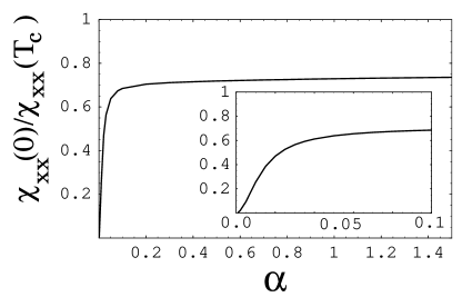
Figure 9: $\chi_{xx}(T=0)/\chi_{xx}(T=T_{c})$ in the superconducting state versus $\alpha$ for the model defined by Eqs.(1), (67), and (68) with $U=0$. Inset: the enlarged plot for small $\alpha$

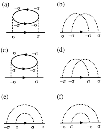
Figure 10: Diagrams for the self-energy on the order of $U^{2}$. Up to this order, the diagram (a) gives the most prominent electron correlation effects. The contributions from the other diagrams are suppressed by factors of order $\sim O(\alpha|\mbox{\boldmath$t$}_{0k}|/E_{F})$

.

Figure 11: $\chi_{xx}(T=0)/\chi_{xx}(T=T_{c})$ in the superconducting state versus $U/W$ with $\alpha=0.5$ (open circles) and $\alpha=1.0$ (crosses) calculated by the second order perturbative expansion with respect to $U$ for the model defined by Eqs.(1), (67), and (68).

III.3 Implication for the Knight shift measurement of CePt₃Si

Here we would like to argue an implication of (130) for CePt₃Si. There are strong pieces of experimental evidence suggesting the realization of an unconventional pairing state in CePt₃Si.yogi ; yogi2 ; matsu ; pene Nevertheless, the symmetry of the Cooper pair has not yet been clarified so far. According to the Knight shift measurements done by Yogi et al.yogi ; yogi2 for this system, both $\chi_{xx}$ and $\chi_{zz}$ does not show any significant change even below the superconducting transition temperature $T_{c}$. The absence of the substantial decrease of $\chi_{xx}$ for $T<T_{c}$ seems not to be consistent with Eq.(130), which indicates the decrease of the Pauli term both in the spin singlet and triplet superconducting states. To resolve this point, we note that the magnitude of the ratio $\chi_{xx}(T=0)/\chi_{xx}(T=T_{c})$ in the superconducting state crucially depends on the details of the electronic structure. For instance, when the density of states has the strong energy-dependence as shown in FIG.7, the value of $\chi_{xx}(T=0)/\chi_{xx}(T=T_{c})$ may deviate from 1/2. To demonstrate this, we use the model considered in Sec.II.C., given by the Hamiltonian (1) with Eqs.(67) and (68) at the half-filling. This model has the density of states similar to that depicted in FIG.7 because of the existence of the van Hove singularity. We chose the magnitude of the superconducting gap as $\Delta_{\pm}\approx 0.01$, and calculate the spin susceptibility at zero temperature from Eq.(130). In FIG.8, we show the plot of $\chi_{xx}(T=0)/\chi_{xx}(T=T_{c})$ versus the strength of the spin-orbit interaction $\alpha$ for the non-interacting case $U=0$. It is seen that, for small $\alpha$, $\chi_{xx}(T=0)/\chi_{xx}(T=T_{c})$ is nearly equal to zero. As $\alpha$ increases, the value of the ratio becomes larger, and eventually goes over $1/2$, because of the enhancement of the density of states due to the van Hove singularity. The maximum value of the ratio is still smaller than the experimentally observed value for CePt₃Si, i.e. $\chi_{xx}(T=0)/\chi_{xx}(T=T_{c})\approx 1$. However, it is expected that if electron correlation effects are included, the van-Vleck-like term enjoys the enormous enhancement caused by the contributions from the van Hove singularity, which is absent for the Pauli term if the spin-orbit splitted Fermi surfaces are sufficiently away from the van Hove points. To confirm this prediction, we carry out the perturbative calculation of the electron correlation effects by expanding the self-energy in terms of the Coulomb interaction $U$ up to the second order. We consider the case where the spin-orbit splitting is much larger than the superconducting gap. Then, $\chi_{xx}(T=0)$ can be well approximated by the van-Vleck-like susceptibility in the normal state. Using the expressions in the normal state Eqs.(61) and (62), we compute numerically the ratio $\chi_{xx}(T=0)/\chi_{xx}(T=T_{c})$ for $\alpha=0.5$ and $\alpha=1.0$. Since the spin-orbit splitting is still much smaller than the band width $W\approx 8$, we neglect corrections of order $O(\alpha|\mbox{\boldmath$t$}_{0k}|/W)$, preserving only the contribution from the diagram FIG.9(a). This amounts to considering only the term proportional to $\partial\Sigma_{x}/\partial(\mu_{\rm B}H_{x})$ in Eqs.(64) and (65). Since the numerical computation of the derivative of the self-energy with respect to a magnetic field is somewhat difficult, we use the approximation $\partial\Sigma_{x}/\partial(\mu_{\rm B}H_{x})\approx\partial\Sigma/\partial(i\varepsilon)$, which is justified when a particular mode of spin fluctuation is not developed, as in the case of CePt₃Si.yy The calculated results of the ratio plotted against $U/W$ are shown in FIG.10. Here $W$ is defined by the average of the band widths of $\varepsilon_{k+}$ and $\varepsilon_{k-}$. As $U/W$ increases, the enhancement of the van-Vleck-like susceptibility due to electron correlation overcomes that of the Pauli term, and the ratio $\chi_{xx}(T=0)/\chi_{xx}(T=T_{c})$ approaches 1.0. Although the strength of the electron-electron interaction for which the ratio is nearly equal to 1.0 is considerably large, we believe that the result obtained by the perturbative calculation may be qualitatively correct, and will be improved by including higher order corrections as long as the system is in the Fermi liquid state. Actually, CePt₃Si is a Fermi liquid with the mass enhancement factor of order $\sim 60$, in which the spin susceptibility is also substantially enhanced. Since we cannot derive such a large mass enhancement from ab initio calculations, we regard the parameter $U$ as an effective interaction renormalized by correlation effects in the above calculations.

Thus, it is possible that for CePt₃Si, the absence of the decrease of $\chi_{xx}(T)$ below $T_{c}$ observed by the NMR experiment may be attributed to a specific energy dependence of the density of states, which leads the existence of the van-Vleck-like term much larger than the Pauli term. Unfortunately, the LDA calculations of the electronic structure of this system done by some groups are restricted within the case without the antiferromagnetic phase transition, which occurs at $T_{N}\sim 2{\rm K}$ in CePt₃Si.hari ; sam Because of this reason, it is difficult to clarify from first principle calculations whether such a strong energy dependence of the density of states exists or or not for CePt₃Si. Experimental studies which directly probe the energy dependence of the density of states for this system are desirable.

III.4 Magnetoelectric effect: Paramagnetic supercurrent

In the absence of inversion symmetry, an intriguing magnetoelectric effect exists in the superconducting state as well as in the normal state, as extensively argued by Edelstein, Yip, and the present author.ede1 ; ede2 ; yip ; fuji2 In the case of the Rashba interaction with a potentail gradient along $\mbox{\boldmath$n$}=(0,0,1)$, an in-plane magnetic field $B$ induces a paramagnetic supercurrent, $\mbox{\boldmath$J$}=\mathcal{K}(\mbox{\boldmath$n$}\times\mbox{\boldmath$B$})$. Here $\mathcal{K}$ is the magnetoelecric effect coefficient, of which the explicit expression including electron correlation effects is presented in ref.fuji2 . The inverse effect is also possible; i.e. the diamagnetic supercurrent flow gives rise to a magnetization.ede2 In the case of the Dresselhaus interaction with $\mbox{\boldmath$\mathcal{L}$}_{0}(k)=(k_{x}(k_{y}^{2}-k_{z}^{2}),k_{y}(k_{z}^{2}-k_{x}^{2}),k_{z}(k_{x}^{2}-k_{y}^{2}))$, a similar effect exists, but the paramagnetic supercurrent flows parallel to the applied magnetic field, $\mbox{\boldmath$J$}=\mathcal{K}\mbox{\boldmath$B$}$, in contrast to the Rashba case where the current flows perpendicular to the magnetic field. The magnetoelectric coefficient $\mathcal{K}$ is also directly related to the stability of the helical vortex phase considered by Kaur et al., and determines the magnitude of the center of mass momentum for inhomogeneous Cooper pairs.kau

Recently, it was pointed out by Yip that the paramagnetic supercurrent is exactly canceled with the magnetization current $\mbox{\boldmath$J$}_{M}=c\nabla\times\mbox{\boldmath$M$}$ in the complete Meissner state in a semi-infinite system.yip2 However, in finite systems, this cancellation is imperfect, and thus the paramagnetic supercurrent gives nonzero contributions to the bulk current. Moreover, in the mixed state, the cancellation is not complete generally. Here we would like to re-examine electron correlation effects on the paramagnetic supercurrent taking into account the partial cancellation with the magnetization current in the case of the Rashba interaction.

Following Yip, we start from the following relations for the supercurrent density $\mbox{\boldmath$J$}_{s}$ and the magnetization density $M$,yip2

$$\mbox{\boldmath$J$}_{s}=\frac{1}{2e\Lambda}(\hbar\nabla\phi-\frac{2e}{c}\mbox{\boldmath$A$})+\mathcal{K}(\mbox{\boldmath$n$}\times\mbox{\boldmath$B$}),$$ (131)

$$\mbox{\boldmath$M$}=\frac{\mathcal{K}}{2e}[\mbox{\boldmath$n$}\times(\hbar\nabla\phi-\frac{2e}{c}\mbox{\boldmath$A$})]+\mbox{\boldmath$M$}_{\rm Zee}.$$ (132)

Here the first term of the right-hand side of Eq.(131) is the diamagnetic supercurrent density which is denoted by $\mbox{\boldmath$J$}^{\rm dia}=(J_{x}^{\rm dia},J_{y}^{\rm dia},J_{z}^{\rm dia})$ in the following. The second term of the right-hand side of (131) is the paramagnetic supercurrent induced by the inversion-symmetry-breaking spin-orbit interaction. The coefficient $1/\Lambda$ of the diamagnetic supercurrent is related to the superfluid density, and equivalent to the Drude weight at zero temperature. The first term of the right-hand side of Eq.(132) is the magnetization induced by the magnetoelectric effect, and the second term $\mbox{\boldmath$M$}_{\rm Zee}$ is a magnetization caused by the usual Zeeman effect. For small $B$, $\mbox{\boldmath$M$}_{\rm Zee}=\chi\mbox{\boldmath$B$}$. Eqs.(131) and (132) are obtained from the free energy in the absence of inversion symmetry as argued by several authors.yip2 ; ede3 ; sam2 ; kau

In addition to the supercurrent $\mbox{\boldmath$J$}_{s}$, there exists the magnetization current density $\mbox{\boldmath$J$}_{M}=c\nabla\times\mbox{\boldmath$M$}$, which is derived by adding the term

$$-\int d\mbox{\boldmath$r$}\mbox{\boldmath$M$}\cdot\mbox{\boldmath$B$}=-\int d\mbox{\boldmath$r$}(\nabla\times\mbox{\boldmath$M$})\cdot\mbox{\boldmath$A$}$$ (133)

to the free energy. Using Eqs.(131), (132), and the relation $\nabla\times\mbox{\boldmath$J$}^{\rm dia}=-\mbox{\boldmath$B$}/(c\Lambda)$, we havevc

$$\mathcal{K}(\mbox{\boldmath$n$}\times\mbox{\boldmath$B$})=-c\nabla\times(\mbox{\boldmath$M$}-\mbox{\boldmath$M$}_{\rm Zee})$$

$$+c\mathcal{K}\Lambda(-\partial_{x}J_{z}^{\rm dia},\partial_{y}J_{z}^{\rm dia},\partial_{x}J_{x}^{\rm dia}+\partial_{y}J_{y}^{\rm dia}).$$ (134)

Then, the total current density $\mbox{\boldmath$J$}_{\rm tot}$ is recast into

$$\mbox{\boldmath$J$}_{\rm tot} = \mbox{\boldmath$J$}_{s}+\mbox{\boldmath$J$}_{M}$$ (135)

$$= \mbox{\boldmath$J$}^{\rm dia}+c\nabla\times\mbox{\boldmath$M$}_{\rm Zee}$$

$$+ c\mathcal{K}\Lambda(-\partial_{x}J_{z}^{\rm dia},\partial_{y}J_{z}^{\rm dia},\partial_{x}J_{x}^{\rm dia}+\partial_{y}J_{y}^{\rm dia}).$$

The second term of the right-hand side of Eq.(135) is the magnetization current caused by the usual Zeeman effect. The last term of Eq.(135) is the paramagnetic supercurrent due to the magnetoelectric effect with which we are concerned. Apparently, this paramagnetic term vanishes in the thermodynamic limit in the complete Meissner state in an infinite $x$-$y$ planar system, as was pointed out by Yip.yip2 Nevertheless, it still plays a crucial role in finite systems in the Meissner state, or generically in the mixed state. Using Eq.(135), we can discuss electron correlation effects on the paramagnetic supercurrent partly canceled with the magnetization current. According to the analysis presented in ref.fuji2 ; add , $\mathcal{K}$ is given by

$$\frac{\mathcal{K}}{e\mu_{\rm B}}=$$

$$\sum_{k}\sum_{\tau=\pm 1}\tau v_{0y\tau}\frac{z_{k\tau}\Delta_{k\tau}^{2}}{E_{k\tau}^{2}}\left[\frac{{\rm ch}^{-2}\frac{E_{k\tau}}{2T}}{2T}-\frac{{\rm th}\frac{E_{k\tau}}{2T}}{E_{k\tau}}\right]\Lambda^{sx}_{\tau}(E_{k\tau},\mbox{\boldmath$k$})$$

$$+2\alpha\sum_{k}\frac{\Delta_{k+}\Delta_{k-}}{E_{k+}^{2}-E_{k-}^{2}}\left[z_{k-}\frac{{\rm th}\frac{E_{k+}}{2T}}{E_{k+}}-z_{k+}\frac{{\rm th}\frac{E_{k-}}{2T}}{E_{k-}}\right]$$

$$\times\hat{t}_{x}\Lambda^{sx}_{+-}(E_{k\tau},\mbox{\boldmath$k$}),$$ (136)

which is enhanced by the factor $1/z_{k\tau}$, when the Wilson ratio is nearly equal to 2, as in the case of typical heavy fermion systems. On the other hand, the coefficient of the diamagnetic supercurrent $1/\Lambda$ is suppressed by the factor $z_{k\tau}$. This fact indicates that the last term of the right-hand side of (135) is enhanced by the factor $1/z_{k\tau}^{2}$ compared to the first term $\mbox{\boldmath$J$}^{\rm dia}$. Thus, even when the partial cancellation with the magnetization current takes place. the paramagnetic supercurrent induced by the magnetoelectric effect is still amplified in strongly correlated electron systems with large mass enhancement. This observation is quite important for the experimental detection of the magnetoelectric effect in heavy fermion superconductors such as CePt₃Si, CeRhSi₃, UIr, and CeIrSi₃.

IV Summary

In this paper, we have explored magnetic properties and transport phenomena in interacting electron systems without inversion symmetry in the normal state as well as in the superconducting state on the basis of the general framework of the Fermi liquid theory, taking into account electron correlation effects in a formally exact way. We have obtained the formulae for the transport coefficients related to the anomalous Hall effect, the thermal anomalous Hall effect, the spin Hall effect, and the magnetoelectric effect, which are the results of the parity violation. It is found that the spin Hall conductivity is not renormalized by electron correlation effects, and is determined solely by the band structure. Also, it is pointed out that in the superconducting state, the thermal anomalous anomalous Hall conductivity divided by the temperature and the magnetic field $\kappa_{xy}^{\rm AHE}/(TH_{z})$ remains finite even in the zero temperature limit, despite the absence of Bogoliubov quasiparticles carrying heat currents. This intriguing property is due to the fact that the anomalous Hall conductivity in the absence of inversion symmetry is dominated by electrons occupying the momentum space sandwiched between the spin-orbit splitted two Fermi surfaces, which are not affected by the superconducting transition. We have also examined electron correlation effects on the paramagnetic supercurrent caused by the magnetoelectric effect taking account of the partial cancellation with the magnetization current. The experimental detection of these effects in the recently discovered noncentrosymmetric heavy fermion superconductors CePt₃Si, UIr, CeRhSi₃, and CeIrSi₃. is an important future issue.

Furthermore, we have demonstrated that in the normal state the temperature dependence of the van-Vleck-like spin susceptibility behaves like the Pauli susceptibility, in contrast to the usual van Vleck orbital susceptibility, and that the ratio of the van-Vleck-like term to the Pauli term depends crucially on the details of the electronic structure and electron correlation effects. This result leads us a possible explanation for the recent NMR experimental data of CePt₃Si, which indicates no change of the Knight shift below $T_{c}$ for any directions of a magnetic field, contrary to previous theoretical predictions.yogi2 It is suggested that the strong energy dependence of the density of states and electron correlation effects may strongly enhance the van-Vleck-like susceptibility compared to the Pauli term, and thus the total spin susceptibility is not much affected by the superconducting transition.

- (1) E. Bauer, G. Hilscher, H. Michor, Ch. Paul, E. W. Scheidt, A. Gribanov, Yu. Seropegin, H. Noël, M. Sigrist, and P. Rogl: Phys. Rev. Lett. 92 (2004) 027003.
- (2) T. Akazawa, H. Hidaka, H. Kotegawa, T. Kobayashi, T. Fujiwara, E. Yamamoto, Y. Haga, R. Settai, and Y. nuki: J. Phys. Soc. Jpn. 73 (2004) 3129.
- (3) N. Kimura, K. Ito, K. Saitoh, Y. Umeda, H. Aoki, and T. Terashima: Phys. Rev. Lett. 95 (2005) 247004.
- (4) I. Sugitani, Y. Okuda, H. Shishido, T. Yamada, A. Thamizhavel, E. Yamamoto, T. D. Matsuda, Y. Haga, T. Takeuchi, R. Settai, and Y. Onuki: J. Phys. Soc. Jpn. 75 (2006) 043703.
- (5) K. Togano, P. Badica, Y. Nakamori, S. Orimo, H. Takeya, and K. Hirata: Phys. Rev. Lett. 93 (2004) 247004.
- (6) P. Badica, T. Kondo, and K. Togano: J. Phys. Soc. Jpn: 74 (2005) 1014.
- (7) V. M. Edelstein: Sov. Phys. JETP 68 (1989) 1244.
- (8) L. P. Gor’kov and E. Rashba: Phys. Rev. Lett. 87 (2001) 037004.
- (9) P. A. Frigeri, D. F. Agterberg, A. Koga, and M. Sigrist: Phys. Rev. Lett. 92 (2004) 097001.
- (10) I. A. Sergienko and S. H. Curnoe: Phys. Rev. B70 (2004) 214510.
- (11) V. M. Edelstein: Phys. Rev. Lett. 75 (1995) 2004.
- (12) V. M. Edelstein: J. Phys. Condens. Matter 8 (1996) 339.
- (13) S. K. Yip: Phys. Rev. B 65 (2002) 144508.
- (14) S. K. Yip: J. Low Temp. Phys. 140 (2005) 67.
- (15) K. Samokhin: Phys. Rev. B70 (2004) 104521.
- (16) R. P. Kaur, D. F. Agterberg, and M. Sigrist: Phys. Rev. Lett.94 (2005) 137002.
- (17) S. Fujimoto: Phys. Rev. B72 (2005) 024515.
- (18) N. Hayashi, K. Wakabayashi, P.A. Frigeri, and M. Sigrist: Phys. Rev. B73 (2006) 092508; ibid 73 (2006) 024504.
- (19) T. Yokoyama, Y. Tanaka, and J. Inoue: Phys. Rev. B 72 (2006) 220504(R).
- (20) M. Oka, M. Ichioka, and K. Machida, Phys. Rev. B73 (2006) 214509.
- (21) L. S. Levitov, Yu. V. Nazarov, an G. M. Eliashberg: Sov. Phys. JETP 61 (1985) 133.
- (22) V. M. Edelstein: Solid State Commun.73 (1990) 233.
- (23) S. Murakami, N. Nagaosa, and S. C. Zhang: Science 301 (2003) 1348.
- (24) J. Sinova, D. Culcer, Q. Niu, N. A. Sinitsyn, T. Jungwirth, and A. H. MacDonald: Phys. Rev. Lett. 92 (2004) 126603.
- (25) R. Karplus and J. M. Luttinger: Phys. Rev. 95 (1954) 1154; J. M. Luttinger: Phys. Rev. 112 (1958) 739.
- (26) T. Jungwirth, Qian Niu, and A. H. MacDonald: Phys. Rev. Lett. 88 (2002) 207208.
- (27) M. Yogi, Y. Kitaoka, S. Hashimoto, T. Yasuda, R. Settai, T. D. Matsuda, Y. Haga, Y. nuki, P. Rogl, and E. Bauer: Phys. Rev. Lett. 93 (2004) 027003.
- (28) M. Yogi, H. Mukuda, Y. Kitaoka, S. Hashimoto, T. Yasuda, R. Settai, T. D. Matsuda, Y. Haga, Y. Onuki, P. Rogl, and E. Bauer: J. Phys. Soc. Jpn. 75 (2006) 013709.
- (29) E. I. Rashba: Sov. Phys. Solid State 2 (1960) 1109.
- (30) G. Dresselhaus: Phys. Rev. 100 (1955) 580.
- (31) M. I. D’Yakonov and V. I. Perel: Sov. Phys. JETP 33 (1971) 1053.
- (32) E. A. de Andrada e Silva: Phys. Rev. B46 (1992) 1921.
- (33) see, e.g., J. R. Schrieffer,Theory of Superconductivity (Addison Wesley, Reading, 1983).
- (34) S. Hashimoto, T. Yasuda, T. Kubo, H. Shishido, T. Ueda, R. Settai, T. D. Matsuda, Y. Haga, H. Harima, and Y. nuki: J. Phys.: Condens. Matter 16 (2004) L287.
- (35) K. V. Samokhin, E. S. Zijlstra, and S. K. Bose, Phys. Rev. B69 (2004) 094514.
- (36) T. Takeuchi, S. Hashimoto, T. Yasuda, H. Shishido, T. Ueda, M. Yamda, Y. Obiraki, M. Shiimoto, H. Kohara, T. Yamamoto, K. Sugiyama, K. Kindo, T. D. Matsuda, Y. Haga, Y. Aoki, H. Sato, R. Settai, and Y. nuki: J. Phys.: Condens. Matter 16 (2004) L333.
- (37) N. Metoki, K. Kaneko, T. D. Matsuda, A. Galatanu, T. Takeuchi, S. Hashimoto, T. Ueda, R. Settai, Y. nuki, and N. Berngoeft: J. Phys.: Condens. Matter 16 (2004) L207.
- (38) M. Hadzic-Leroux, A. Hamzic, A. Fert, P. Haen, F. Lapierre, and O. Laborde: Europhys. Lett. 1 (1986) 579.
- (39) P. Coleman, P. W. Anderson, and T. V. Ramakrishnan: Phys. Rev. Lett. 55 (1985) 414.
- (40) A. Fert and P. M. Levy: Phys. Rev. B36 (1987) 1907.
- (41) H. Kohno and K. Yamada: J. Magn. & Magn. Mater. 90&91 (1990) 431.
- (42) H. Kontani and K. Yamada: J. Phys. Soc. Jpn. 63 (1994) 2627.
- (43) K. Yamada and K. Yosida: Prog. Thoer. Phys. 76 (1986) 621.
- (44) G. M. Eliashberg: Sov. Phys. JETP 14 (1962) 886.
- (45) N. Kimura, Y. Umeda, T. Asai, T. Terashima, and H. Aoki: Physica B294-295 (2001) 280.
- (46) A. J. Leggett: Phys. Rev. 140 (1965) 1869; Phys. Rev. 147 (1966) 119.
- (47) A. I. Larkin and A. B. Migdal: Sov. Phys. JETP 17 (1963) 1146.
- (48) S. Fujimoto: J. Phys. Soc. Jpn.61 (1992) 765.
- (49) The expression of given in ref.fuji2 should be amended as Eq.(130) in the present paper.
- (50) K. Izawa, Y. Kasahara, Y. Matsuda, K. Behnia, T. Yasuda, R. Settai, and Y. nuki: Phys. Rev. Lett. 94 (2005) 197002.
- (51) I. Bonalde, W. Brämer-Escamilla, and E. Bauer: Phys. Rev. Lett. 94 (2005) 207002.
- (52) In the case of the mixed state, naturally, this argument is applied only to the region outside of vortex cores.
- (53) In ref.fuji2 , the final expression of (Eq.(36) in ref.fuji2 ) should be amended as Eq.(136) in the present paper, because, in ref.fuji2 , the quasiparticle approximation was erroneously applied to the energy region away from the Fermi level. This correction does not flaw the main conclusion of ref.fuji2 , but rather justifies its validity.