A theory of the electric quadrupole contribution to resonant x-ray scattering:
Application to multipole ordering phases in Ce_1-xLa_xB₆

Abstract

We study the electric quadrupole ($E$2) contribution to resonant x-ray scattering (RXS). Under the assumption that the rotational invariance is preserved in the Hamiltonian describing the intermediate state of scattering, we derive a useful expression for the RXS amplitude. One of the advantages the derived expression possesses is the full information of the energy dependence, lacking in all the previous studies using the fast collision approximation. The expression is also helpful to classify the spectra into multipole order parameters which are brought about. The expression is suitable to investigate the RXS spectra in the localized $f$ electron systems. We demonstrate the usefulness of the formula by calculating the RXS spectra at the Ce $L_{2,3}$ edges in Ce_1-xLa_xB₆ on the basis of the formula. We obtain the spectra as a function of energy in agreement with the experiment of Ce_0.7La_0.3B₆. Analyzing the azimuthal angle dependence, we find the sixfold symmetry in the $\sigma$-$\sigma^{\prime}$ channel and the threefold one in the $\sigma$-$\pi^{\prime}$ channel not only in the antiferrooctupole (AFO) ordering phase but also in the antiferroquadrupole (AFQ) ordering phase, which behavior depends strongly on the domain distribution. The sixfold symmetry in the AFQ phase arises from the simultaneously induced hexadecapole order. Although the AFO order is plausible for phase IV in Ce_1-xLa_xB₆, the possibility of the AFQ order may not be ruled out on the basis of azimuthal angle dependence alone.

I Introduction

Resonant x-ray scattering (RXS) has recently attracted much attention, since strong x-ray intensities have become available from the synchrotron radiation. It is described by a second-order process that a core electron is excited into unoccupied states by absorbing incident x-rays and that electron is recombined with the core hole by emitting x-rays. The RXS has been recognized as a useful probe to investigate spatially varying multipole orderings, which the conventional neutron scattering is usually difficult to detect.

For probing the spacial variation of order parameters, x-ray wavelengths need to be order of the variation period. In transition metals, the $K$ edges in the dipole ($E$1) transition are just fitting for this purpose. Actually, by using the $K$ edge, the possibility of the orbital ordering has already been explored in transition-metal compounds. Murakami et al. (1998a, b) The RXS intensities are observed at superlattice Bragg spots, which are interpreted as originating from the modulation in the $4p$ band, since the process involves the excitation of a $1s$ electron to unoccupied $4p$ states.

Because the ordering pattern is usually controlled by electrons in the $3d$ band, the mechanism which causes the modulation is not necessarily trivial. Actually, for most of transition-metal compounds, both experimental studies and theoretical studies based on electronic structure calculations have revealed that the RXS intensities are brought about by the hybridization between the $4p$ band and the $2p$ band of the neighboring anions rather than the direct Coulomb interaction between the electron in the $4p$ band and electrons in the $3d$ band.Ohsumi et al. (2003); Igarashi and Takahashi (2005) This result is reasonable because of the extended nature of the $4p$ state.

On rare earth metal compounds such as CeB₆, DyB₂C₂, the $L_{2,3}$ edges in the $E$1 transition are used because of the requirement for x-ray wavelength. Nakao et al. (2001); Yakhou et al. (2001); Hirota et al. (2000); Tanaka et al. (1999) The RXS spectra in the $E$1 transition from the antiferroquadrupole (AFQ) phase of CeB₆ were studied both experimentallyNakao et al. (2001) and theoretically.Nagao and Igarashi (2001); Igarashi and Nagao (2002) Although the experiments and the theory give sufficiently consistent results, the relation to the multipole orderings which $4f$ electrons mainly involve is rather indirect, since the resonance is caused by the excitation of a $2p$ electron to $5d$ states. This shortcoming may be overcome by using the quadrupole ($E$2) transition at the $L_{2,3}$ edges, where a $2p$ electron is promoted to partially filled $4f$ states. Using the $E$2 transition has another merit that octupole and hexadecapole orderings are directly detectable. This contrasts with the $E$1 transition, where only dipole and quadrupole orderings are detectable. Of course, intensities in the $E$2 transition are usually much smaller than those in the $E$1 transition.

In this paper, we derive a general formula of the RXS amplitudes in the localized electron picture, in which the electronic structure at each atom is assumed to be well described by an atomic wavefunction under the crystal electric field (CEF). Historically, the research in such a direction was started by using the framework borrowed from resonant $\gamma$-ray scattering.Trammel (1962) Starting from the works by Blume and GibbsBlume and Gibbs (1988) and by Hannon et al.Hannon et al. (1989), the form of the RXS amplitude had been investigated in several works.Luo et al. (1993); Carra and Thole (1994); Lovesey and Balcar (1996); Hill and McMorrow (1996) The RXS amplitude can be summarized into an elegant form by using vector spherical harmonics. Unfortunately, it has little practical usage because it is difficult to deduce meaningful information when there is no restriction on the intermediate state of the scattering process. A widely-adopted approximation for practical use is the so-called ”fast collision (FC) approximation”. This replaces the intermediate state energy in the energy denominator of the RXS amplitude by an averaged value, allowing the denominator out of the summation. Hannon et al. (1989); Luo et al. (1993); Carra and Thole (1994); Lovesey and Balcar (1996); Hill and McMorrow (1996) Thereby, the multiplet splitting of the intermediate state is neglected, leading to an assumed form (usually a Lorentzian form) for the energy profile.

However, recent experiments show deviation from the Lorentzian form in several materials.Paixão et al. (2002); Wilkins et al. (2004) We improve the situation by taking the energy dependence of the intermediate state under the assumption that the intermediate Hamiltonian describing the scattering process preserves spherical symmetry. This assumption is justified when the CEF energy and the intersite interaction are much smaller than the multiplet energy in the intermediate state as is expected in many localized electron materials. We have already reported the formula for the $E$1 transition, having successfully applied to the analysis of the $E$1 RXS spectra in URu₂Si₂ and NpO₂.Nagao and Igarashi (2005a, b, ) This paper is an extension of those works to the $E$2 transition. The obtained formula makes it possible to analyze the energy profiles of the spectra in contrast with the FC approximation. In addition, the formula is suitable to discuss the relation of the RXS spectra to multipole order parameters, Isaacs et al. (1990); Paixão et al. (2002); Bernhoeft et al. (2003); Wilkins et al. (2004); Mannix et al. (2005); Wilkins et al. (2006) because it is expressed by means of the expectation values of the multipole order parameters.

We demonstrate the usefulness of the formula by calculating the RXS spectra in multipole ordering phases of Ce_1-xLa_xB₆. First, we investigate the $E$2 RXS spectra at the Ce $L_{2,3}$ edges from the AFQ ordering phase (phase II) in the non-diluted material CeB₆. Analysis utilizing our formula reveals that the $E$2 RXS spectra in phase II consist of a mixture of the quadrupole and hexadecapole energy profiles. The calculated intensities suggest the possibility that he $E$2 signal at the Ce $L_{2,3}$ edges can be detectable in this material.

For the intermediate doping range $x\approx 0.3\sim 0.5$, Ce_1-xLa_xB₆ falls into a new phase (phase IV) whose primary order parameter is not well established yet.Tayama et al. (1997) Recently, the $E$2 RXS signals at the Ce $L_{2}$ edge have been detected for an $x=0.3$ sample.Mannix et al. (2005) From the azimuthal angle ($\psi$) dependence of the peak intensity, it was claimed that the antiferrooctupole (AFO) ordering phase is the most probable candidate because the symmetry of the $\psi$-dependence, sixfold and threefold in the $\sigma$-$\sigma^{\prime}$ and $\sigma$-$\pi^{\prime}$ channels respectively, is deduced from the theory in good agreement with the experiment.Mannix et al. (2005); Kusunose and Kuramoto (2005) However, the relative intensity between two channels depends strongly on the domain distribution, and deviates about factor two from the experimental one if the contribution from four domains are added with equal weight. The origin of this discrepancy is still unanswered. It will be pointed out that the RXS peak intensity from the AFQ phase concomitant with the induced hexadecapole contribution also gives rise to the same symmetry of the $\psi$-dependence as obtained from the AFO phase. Thus, although the AFO order is plausible in many respects, it seems difficult to rule out the AFQ order on the basis of the azimuthal angle dependence alone. In addition, we calculate the energy dependence of the RXS spectra at the Ce $L_{2,3}$ edges. Assuming both the AFO and AFQ orders, we obtain the spectral shapes at the $L_{2}$ edge, which agree with the experimental one for Ce_0.7La_0.3B₆.Mannix et al. (2005) On the other hand, the spectral shapes at the $L_{3}$ edge are found slightly different between two phases, with intensities the same order of magnitude of the reported one at the $L_{2}$ edge.

The present paper is organized as follows. A general expression for RXS amplitudes is obtained in Sec. II. Analysis of RXS spectra in Ce_1-xLa_xB₆ are presented in Sec. III. Section IV is devoted to concluding remarks. In Appendix, we show several expressions required to obtain the RXS amplitude formula.

II Theoretical Framework of RXS

II.1 a second-order optical process

The RXS is described by a second-order optical process, where a core electron is excited to unoccupied states by absorbing x-rays and that electron is recombined with the core hole by emitting x-rays. Since the wavefunction of core electron is well localized, the RXS amplitude may be given by a sum of contributions from individual ions. Using a geometrical arrangement shown in Fig. 1, we express the RXS amplitude $f(\mbox{\boldmath{$\epsilon$}},\mbox{\boldmath{$\epsilon$}}^{\prime},{\textbf{k}},{\textbf{k}}^{\prime},\omega)$ for the incident x-ray with momentum k, polarization $\epsilon$, and the scattered x-ray with momentum ${\textbf{k}}^{\prime}$, polarization $\mbox{\boldmath{$\epsilon$}}^{\prime}$ as

$$f(\mbox{\boldmath{$\epsilon$}},\mbox{\boldmath{$\epsilon$}}^{\prime},{\textbf{k}},{\textbf{k}}^{\prime},\omega) = \sum_{n=1}f^{(n)}(\mbox{\boldmath{$\epsilon$}},\mbox{\boldmath{$\epsilon$}}^{\prime},{\textbf{k}},{\textbf{k}}^{\prime},\omega),$$ (1)

$$f^{(n)}(\mbox{\boldmath{$\epsilon$}},\mbox{\boldmath{$\epsilon$}}^{\prime},{\textbf{k}},{\textbf{k}}^{\prime},\omega) \propto \frac{1}{\sqrt{N}}\sum_{j}{\textrm{e}}^{-i{\textbf{G}}\cdot{\textbf{r}}_{j}}$$ (2)

$$\times M_{j}^{(n)}(\mbox{\boldmath{$\epsilon$}},\mbox{\boldmath{$\epsilon$}}^{\prime},{\textbf{k}},{\textbf{k}}^{\prime},\omega),$$

with

$$M_{j}^{(1)}(\mbox{\boldmath{$\epsilon$}},\mbox{\boldmath{$\epsilon$}}^{\prime},\omega) = \sum_{\mu,\mu^{\prime}}\epsilon^{\prime}_{\mu}\epsilon_{\mu^{\prime}}$$ (3)

$$\times \sum_{\Lambda}\frac{\langle\psi_{0}|x_{\mu,j}|\Lambda\rangle\langle\Lambda|x_{\mu^{\prime},j}|\psi_{0}\rangle}{\hbar\omega-(E_{\Lambda}-E_{0})+i\Gamma},$$

$$M_{j}^{(2)}(\mbox{\boldmath{$\epsilon$}},\mbox{\boldmath{$\epsilon$}}^{\prime},{\textbf{k}},{\textbf{k}}^{\prime},\omega) = \frac{k^{2}}{9}\sum_{\mu,\mu^{\prime}}q_{\mu}(\hat{\bf k}^{\prime},\mbox{\boldmath{$\epsilon$}}^{\prime})q_{\mu^{\prime}}(\hat{\bf k},\mbox{\boldmath{$\epsilon$}})$$ (4)

$$\times \sum_{\Lambda}\frac{\langle\psi_{0}|\tilde{z}_{\mu,j}|\Lambda\rangle\langle\Lambda|\tilde{z}_{\mu^{\prime},j}|\psi_{0}\rangle}{\hbar\omega-(E_{\Lambda}-E_{0})+i\Gamma},$$

where G ($={\textbf{k}}^{\prime}-{\textbf{k}}$) is the scattering vector, and $N$ is the number of sites $j$’s. The $|\psi_{0}\rangle$ represents the ground state with energy $E_{0}$, while $|\Lambda\rangle$ represents the intermediate state with energy $E_{\Lambda}$. The $\Gamma$ describes the life-time broadening width of the core hole. Equation (3) describes the $E$1 transition, where the dipole operators $x_{\mu,j}$’s are defined as $x_{1,j}=x_{j}$, $x_{2,j}=y_{j}$, and $x_{3,j}=z_{j}$ in the coordinate frame fixed to the crystal axes with the origin located at the center of site $j$. Equation (4) describes the $E$2 transition, where the quadrupole operators are defined by $\tilde{z}_{1,j}=\frac{\sqrt{3}}{2}(x_{j}^{2}-y_{j}^{2})$, $\tilde{z}_{2,j}=\frac{1}{2}(3z_{j}^{2}-r_{j}^{2})$, $\tilde{z}_{3,j}=\sqrt{3}y_{j}z_{j}$, $\tilde{z}_{4,j}=\sqrt{3}z_{j}x_{j}$ and $\tilde{z}_{5,j}=\sqrt{3}x_{j}y_{j}$. Factors $q_{\mu}(\hat{\bf k},\mbox{\boldmath{$\epsilon$}})$ and $q_{\mu}(\hat{\bf k}^{\prime},\mbox{\boldmath{$\epsilon$}}^{\prime})$ with $\hat{\textbf{k}}={\textbf{k}}/|{\textbf{k}}|$ and $\hat{\textbf{k}}^{\prime}={\textbf{k}}^{\prime}/|{\textbf{k}}^{\prime}|$ are defined as a second-rank tensor,

$$q_{\mu}({\textbf{A}},{\textbf{B}})\equiv\left\{\begin{array}[]{ll}\frac{\sqrt{3}}{2}\left(A_{x}B_{x}-A_{y}B_{y}\right)&\textrm{for}\ \mu=1,\\ \frac{1}{2}\left(3A_{z}B_{z}-{\textbf{A}}\cdot{\textbf{B}}\right)&\textrm{for}\ \mu=2,\\ \frac{\sqrt{3}}{2}\left(A_{y}B_{z}+A_{z}B_{y}\right)&\textrm{for}\ \mu=3,\\ \frac{\sqrt{3}}{2}\left(A_{z}B_{x}+A_{x}B_{z}\right)&\textrm{for}\ \mu=4,\\ \frac{\sqrt{3}}{2}\left(A_{x}B_{y}+A_{y}B_{x}\right)&\textrm{for}\ \mu=5.\\ \end{array}\right.$$ (5)

Note that the quadrupole operators $\tilde{z}_{\mu,j}$ are expressed as $\tilde{z}_{\mu,j}=q_{\mu}({\textbf{r}}_{j},{\textbf{r}}_{j})$.

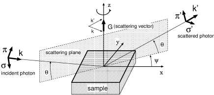
Figure 1: Geometry of the RXS experiment. Photon with polarization $\sigma$ or $\pi$ is scattered into the state of polarization $\sigma^{\prime}$ or $\pi^{\prime}$ at the Bragg angle $\theta$. The azimuthal angle $\psi$ describes the rotation of the sample around the scattering vector G. The $(11\overline{2})$ surface is in the scattering plane at $\psi=0$.

II.2 Energy profiles

In localized electron systems, the ground state and the intermediate state are described in terms of the eigenfunctions of the angular momentum operator, $|J,m\rangle$, at each site. At the ground state, the CEF and the intersite interaction usually lift the degeneracy with respect to $m$. We write the ground state at site $j$ as

$$|\psi_{0}\rangle_{j}=\sum_{m}c_{j}(m)|J,m\rangle.$$ (6)

In the intermediate state, however, the CEF and the intersite interaction may be neglected in a good approximation, since their magnitudes of energy are much smaller than those of the intra-atomic Coulomb interaction and the spin-orbit interaction (SOI) which give rise to the multiplet structure. Thus the Hamiltonian describing the intermediate state is approximated as preserving the spherical symmetry. In such a circumstance, the intermediate states are characterized by the total angular momentum at the core-hole site, that is, $|\Lambda\rangle=|J^{\prime},M,i\rangle$ with the magnitude $J^{\prime}$ and the magnetic quantum number $M$. The corresponding energy is denoted by $E_{J^{\prime},i}$, where we introduce the index $i$ in order to distinguish multiplets having the same $J^{\prime}$ value but having different energy.

In the following, we discuss only on the $E$2 transition (Eq. (4)), because the $E$1 transition has been fully analyzed in our previous paper.Nagao and Igarashi (2005b) First, we rewrite Eq. (4) as

$$M_{j}^{(2)}(\mbox{\boldmath{$\epsilon$}},\mbox{\boldmath{$\epsilon$}}^{\prime},{\textbf{k}},{\textbf{k}}^{\prime},\omega) = \frac{k^{2}}{9}\sum_{\mu,\mu^{\prime}}q_{\mu}(\hat{\textbf{k}}^{\prime},\mbox{\boldmath{$\epsilon$}}^{\prime})q_{\mu^{\prime}}(\hat{\textbf{k}},\mbox{\boldmath{$\epsilon$}})M_{\mu\mu^{\prime}}^{(2)}(\omega,j),$$

$$M_{\mu\mu^{\prime}}^{(2)}(\omega,j) \equiv \sum_{J^{\prime},M,i}E_{i}(\omega,J^{\prime})\langle\psi_{0}|\tilde{z}_{\mu,j}|J^{\prime},M,i\rangle$$ (8)

$$\times \langle J^{\prime},M,i|\tilde{z}_{\mu^{\prime},j}|\psi_{0}\rangle,$$

with

$$E_{i}(\omega,J^{\prime})=\frac{1}{\hbar\omega-(E_{J^{\prime},i}-E_{0})+i\Gamma}.$$ (9)

Then, inserting Eq. (6) for the ground state into Eq. (8), we obtain

$${M}_{\mu\mu^{\prime}}^{(2)}(j,\omega)=\sum_{m,m^{\prime}}c^{\ast}_{j}(m)c_{j}(m^{\prime}){M}_{\mu\mu^{\prime}}^{(2)m,m^{\prime}}(\omega),$$ (10)

with

$${M}_{\mu\mu^{\prime}}^{(2)m,m^{\prime}}(\omega) = \sum_{J^{\prime}}\sum_{i=1}^{N_{J^{\prime}}}E_{i}(\omega,J^{\prime})$$ (11)

$$\times\sum_{M=-J^{\prime}}^{J^{\prime}}\langle J,m|\tilde{z}_{\mu}|J^{\prime},M,i\rangle\langle J^{\prime},M,i|\tilde{z}_{\mu^{\prime}}|J,m^{\prime}\rangle.$$

We have suppressed the index $j$ specifying the core-hole site. The number of the multiplets having the value $J^{\prime}$ is denoted by $N_{J^{\prime}}$. The selection rule for the $E$2 transition confines the range of the summation over $J^{\prime}$ to $J^{\prime}=J,J\pm 1,J\pm 2$.

Now we analyze the matrix element of the type $\langle J,m|\tilde{z}_{\mu}|J^{\prime},M\rangle$ by utilizing the Wigner-Eckart (WE) theorem for a tensor operator,Messiah (1962)

$$\langle J,m|s_{\mu}|J^{\prime}M\rangle = (-1)^{J^{\prime}+m-2}\sqrt{2J+1}$$ (14)

$$\times \left(\begin{array}[]{ccc}J^{\prime}&2&J\\ M&\mu&-m\end{array}\right)(J||V_{2}||J^{\prime}),$$

with $s_{\pm 2}=(\tilde{z}_{1}\pm{\textrm{i}}\tilde{z}_{5})/\sqrt{2}$, $s_{\pm 1}=\mp(\tilde{z}_{4}\pm{\textrm{i}}\tilde{z}_{3})/\sqrt{2}$ and $s_{0}=\tilde{z}_{2}$. The symbol $(J||V_{2}||J^{\prime})$ denotes the reduced matrix element of the set of irreducible tensor operator of the second rank. Because of the nature of the quadrupole operators, a condition $|m-m^{\prime}|\leq 4$ has to be satisfied for non-vanishing ${M}_{\mu\mu^{\prime}}^{(2)m,m^{\prime}}(\omega)$. After a straightforward but tedious calculation with the help of the WE theorem, we obtain non-zero ${M}^{(2)m,m^{\prime}}(\omega)$’s. Then, we perform the summation over $m$ and $m^{\prime}$ in Eq. (10). The result is summarized by introducing the expectation values of the components of the multipole operators as follows:

$$M_{\mu,\mu^{\prime}}^{(2)}(j,\omega)=\sum_{\nu=0}^{4}\alpha_{E2}^{(\nu)}(\omega)\sum_{\lambda=1}^{2\nu+1}[M_{\lambda}^{(\nu)}]_{\mu,\mu^{\prime}}\langle\psi_{0}|z_{\lambda}^{(\nu)}|\psi_{0}\rangle,$$ (15)

where the $\lambda$ th component of rank $\nu$ tensor $z_{\lambda}^{(\nu)}$ in real basis ($1\leq\lambda\leq 2\nu+1$) is defined in Table 1. The $z_{\lambda}^{(\nu)}$ is constructed from the irreducible spherical tensor $T_{\lambda}^{(n)}$ through the unitary transformation $U^{(\nu)}$. The definitions of $T_{n}^{(\nu)}$ and $U^{(\nu)}$ as well as the energy profile $\alpha_{E2}^{(\nu)}(\omega)$ are given in Appendix A. The matrix element of $M_{\lambda}^{(\nu)}$ is expressed as

$$[M_{\lambda}^{(\nu)}]_{\mu,\mu^{\prime}} = \frac{(-)^{\nu}}{(2||T_{\nu}||2)}\sqrt{\frac{2\nu+1}{5}}\sum_{\ell=-2}^{2}\sum_{\ell^{\prime}=-2}^{2}U_{\mu\ell}^{(2)}$$ (18)

$$\times \sum_{n=-\nu}^{\nu}U_{\lambda n}^{(\nu)}([T_{n}^{(\nu)}]_{\ell\ell^{\prime}})^{\ast}[U^{(2)\dagger}]_{\ell^{\prime}\mu^{\prime}}$$

$$= (-)^{\nu}\sqrt{2\nu+1}\sum_{\ell=-2}^{2}\sum_{\ell^{\prime}=-2}^{2}(-)^{\ell}U_{\mu\ell}^{(2)}$$

$$\times \sum_{n=-\nu}^{\nu}U_{\lambda n}^{(\nu)}\left(\begin{array}[]{ccc}2&\nu&2\\ \ell^{\prime}&n&-\ell\\ \end{array}\right)[U^{(2)\dagger}]_{\ell^{\prime}\mu^{\prime}},$$

with

$$(2||T_{\nu}||2)=\frac{1}{2^{\nu}}\sqrt{\frac{(5+\nu)!}{5(4-\nu)!}}.$$ (20)

Table 1: Definition of the operator equivalence of the multipole order components. The overline denotes the symmetrization, for instance, $\overline{X^{2}Y}=X^{2}Y+XYX+YX^{2}$.

$z_{1}^{(1)}=J_{x}$

$z_{2}^{(1)}=J_{y}$

$z_{3}^{(1)}=J_{z}$

$z_{1}^{(2)}=O_{x^{2}-y^{2}}=\frac{\sqrt{3}}{2}[J_{x}^{2}-J_{y}^{2}]$

$z_{2}^{(2)}=O_{3z^{2}-r^{2}}=\frac{1}{2}[3J_{z}^{2}-J(J+1)]$

$z_{3}^{(2)}=O_{yz}=\frac{\sqrt{3}}{2}[J_{y}J_{z}+J_{z}J_{y}]$

$z_{4}^{(2)}=O_{zx}=\frac{\sqrt{3}}{2}[J_{z}J_{x}+J_{x}J_{z}]$

$z_{5}^{(2)}=O_{xy}=\frac{\sqrt{3}}{2}[J_{x}J_{y}+J_{y}J_{x}]$

$z_{1}^{(3)}=T_{xyz}=\frac{\sqrt{15}}{6}\overline{J_{x}J_{y}J_{z}}$

$z_{2}^{(3)}=T_{x}^{\alpha}=\frac{1}{2}[2J_{x}^{3}-\overline{J_{x}(J_{y}^{2}+J_{z}^{2})}]$

$z_{3}^{(3)}=T_{y}^{\alpha}=\frac{1}{2}[2J_{y}^{3}-\overline{J_{y}(J_{z}^{2}+J_{x}^{2})}]$

$z_{4}^{(3)}=T_{z}^{\alpha}=\frac{1}{2}[2J_{z}^{3}-\overline{J_{z}(J_{x}^{2}+J_{y}^{2})}]$

$z_{5}^{(3)}=T_{x}^{\beta}=\frac{\sqrt{15}}{6}\overline{J_{x}(J_{y}^{2}-J_{z}^{2})}$

$z_{6}^{(3)}=T_{y}^{\beta}=\frac{\sqrt{15}}{6}\overline{J_{y}(J_{z}^{2}-J_{x}^{2})}$

$z_{7}^{(3)}=T_{z}^{\beta}=\frac{\sqrt{15}}{6}\overline{J_{z}(J_{x}^{2}-J_{y}^{2})}$

$z_{1}^{(4)}=H_{4}^{0}=\frac{5}{4}\sqrt{\frac{7}{3}}\left[J_{x}^{4}+J_{y}^{4}+J_{z}^{4}-\frac{3}{5}J(J+1)\left\{J(J+1)-\frac{1}{3}\right\}\right]$

$z_{2}^{(4)}=H_{4}^{2}=-\frac{\sqrt{5}}{4}\left[\frac{7}{6}\overline{(J_{x}^{2}-J_{y}^{2})J_{z}^{2}}-\left\{J(J+1)-\frac{5}{6}\right\}(J_{x}^{2}-J_{y}^{2})\right]$

$z_{3}^{(4)}=H_{4}^{4}=\frac{\sqrt{5}}{48}\left[35J_{z}^{4}-30J(J+1)J_{z}^{2}+3J(J+1)[J(J+1)-2]\right.$

$\left.+25J_{z}^{2}-7[J_{x}^{4}+J_{y}^{4}-\overline{J_{x}^{2}J_{y}^{2}}]\right]$

$z_{4}^{(4)}=H_{x}^{\alpha}=\frac{\sqrt{35}}{8}[\overline{J_{y}^{3}J_{z}}-\overline{J_{y}J_{z}^{3}}]$

$z_{5}^{(4)}=H_{y}^{\alpha}=\frac{\sqrt{35}}{8}[\overline{J_{z}^{3}J_{x}}-\overline{J_{z}J_{x}^{3}}]$

$z_{6}^{(4)}=H_{z}^{\alpha}=\frac{\sqrt{35}}{8}[\overline{J_{x}^{3}J_{y}}-\overline{J_{x}J_{y}^{3}}]$

$z_{7}^{(4)}=H_{x}^{\beta}=\frac{\sqrt{5}}{8}[2\overline{J_{x}^{2}J_{y}J_{z}}-(\overline{J_{y}^{3}J_{z}}+\overline{J_{y}J_{z}^{3}})]$

$z_{8}^{(4)}=H_{y}^{\beta}=\frac{\sqrt{5}}{8}[2\overline{J_{y}^{2}J_{z}J_{x}}-(\overline{J_{z}^{3}J_{x}}+\overline{J_{z}J_{x}^{3}})]$

$z_{9}^{(4)}=H_{z}^{\beta}=\frac{\sqrt{5}}{8}[2\overline{J_{z}^{2}J_{x}J_{y}}-(\overline{J_{z}^{3}J_{y}}+\overline{J_{x}J_{y}^{3}})]$

Finally, inserting Eq. (15) into Eq. (LABEL:eq.amplitude.E2.1.5) and using Eq. (LABEL:eq.m.matrix), we obtain the final expression,

$$M_{j}^{(2)}(\mbox{\boldmath{$\epsilon$}},\mbox{\boldmath{$\epsilon$}}^{\prime},{\textbf{k}},{\textbf{k}}^{\prime},\omega)$$

$$= \frac{k^{2}}{9}\sum_{\nu=0}^{4}\alpha_{E2}^{(\nu)}(\omega)\sum_{\lambda=1}^{2\nu+1}P_{\lambda}^{(\nu)}(\mbox{\boldmath{$\epsilon$}},\mbox{\boldmath{$\epsilon$}}^{\prime},\hat{\textbf{k}},\hat{\textbf{k}}^{\prime})\langle\psi_{0}|z_{\lambda}^{(\nu)}|\psi_{0}\rangle,$$

where $P_{\lambda}^{(\nu)}$’s are the geometrical factors defined as

$$P_{\lambda}^{(\nu)}(\mbox{\boldmath{$\epsilon$}},\mbox{\boldmath{$\epsilon$}}^{\prime},\hat{\textbf{k}},\hat{\textbf{k}}^{\prime})$$ (24)

$$= \sqrt{2\nu+1}\sum_{n=-\nu}^{\nu}(-)^{n}U_{\lambda n}^{(\nu)}\sum_{m=-\nu}^{\nu}\left(\begin{array}[]{ccc}2&2&\nu\\ m&n-m&-n\\ \end{array}\right)$$

$$\times q_{m}(\mbox{\boldmath{$\epsilon$}}^{\prime},\hat{\textbf{k}}^{\prime})q_{n-m}(\mbox{\boldmath{$\epsilon$}},\hat{\textbf{k}}).$$ (25)

Those for $\nu=0,1$ and $2$ are expressed as relatively simple forms:

$$P_{1}^{(0)}(\mbox{\boldmath{$\epsilon$}},\mbox{\boldmath{$\epsilon$}}^{\prime},{\textbf{k}},{\textbf{k}}^{\prime}) = \frac{1}{\sqrt{5}}\left[(\hat{\textbf{k}}^{\prime}\cdot\hat{\textbf{k}})(\mbox{\boldmath{$\epsilon$}}^{\prime}\cdot\mbox{\boldmath{$\epsilon$}})+(\hat{\textbf{k}}^{\prime}\cdot\mbox{\boldmath{$\epsilon$}})(\mbox{\boldmath{$\epsilon$}}^{\prime}\cdot\hat{\textbf{k}})\right],$$

$$P_{\mu}^{(1)}(\mbox{\boldmath{$\epsilon$}},\mbox{\boldmath{$\epsilon$}}^{\prime},\hat{\textbf{k}},\hat{\textbf{k}}^{\prime})$$ (27)

$$=-{\textrm{i}}\frac{1}{\sqrt{10}}\left[(\mbox{\boldmath{$\epsilon$}}^{\prime}\cdot\mbox{\boldmath{$\epsilon$}})(\hat{\textbf{k}}^{\prime}\times\hat{\textbf{k}})_{\mu}+(\hat{\textbf{k}}^{\prime}\cdot\hat{\textbf{k}})(\mbox{\boldmath{$\epsilon$}}^{\prime}\times\mbox{\boldmath{$\epsilon$}})_{\mu}\right.$$

$$\left.+({\textrm{k}}^{\prime}\cdot\mbox{\boldmath{$\epsilon$}})(\mbox{\boldmath{$\epsilon$}}^{\prime}\times\hat{\textbf{k}})_{\mu}+(\mbox{\boldmath{$\epsilon$}}^{\prime}\cdot\hat{\textbf{k}})(\hat{\textbf{k}}^{\prime}\times\mbox{\boldmath{$\epsilon$}})_{\mu},\right],$$

$$P_{\mu}^{(2)}(\mbox{\boldmath{$\epsilon$}},\mbox{\boldmath{$\epsilon$}}^{\prime},\hat{\textbf{k}},\hat{\textbf{k}}^{\prime}) = -\frac{3}{2}\frac{1}{\sqrt{14}}\left[(\mbox{\boldmath{$\epsilon$}}^{\prime}\cdot\mbox{\boldmath{$\epsilon$}})q_{\mu}(\hat{\textbf{k}},\hat{\textbf{k}}^{\prime})\right.$$ (28)

$$\left.+(\hat{\textbf{k}}^{\prime}\cdot\hat{\textbf{k}})q_{\mu}(\mbox{\boldmath{$\epsilon$}},\mbox{\boldmath{$\epsilon$}}^{\prime})+q_{\mu}(\hat{\textbf{k}}^{\prime}\times\hat{\textbf{k}},\mbox{\boldmath{$\epsilon$}}^{\prime}\times\mbox{\boldmath{$\epsilon$}})\right].$$

For $\nu=1$, indices $\mu=1,2$ and $3$ serve as the Cartesian components $x,y$ and $z$, respectively. The corresponding expression of $P_{\mu}^{(\nu)}$’s for $\nu=3,4$ have complicated forms, which are summarized in Appendix B.

An expression similar to Eq. (LABEL:eq.amplitude.E2.final) has been derived by the FC approximation. Hannon et al. (1989); Luo et al. (1993); Carra and Thole (1994); Hill and McMorrow (1996); Lovesey and Balcar (1996) However, this scheme has to put by hand the energy dependence. The present theory gives an explicit expression of the energy dependence, which is separated from the factor relating to the order parameter. Thus, the choice of the CEF parameters in the ground state does not affect the shape of energy profiles $\alpha_{E2}^{(\nu)}(\omega)$.

III Application to multipole ordering phases in Ce_1-xLa_xB₆

In this section, we demonstrate the usefulness of Eq.(LABEL:eq.amplitude.E2.final) by analyzing the RXS spectra in the $E$2 transition at the Ce $L_{2,3}$ edges from Ce_1-xLa_xB₆.

III.1 Phase II in CeB₆

The parent material CeB₆ experiences two-step phase transitions. It undergoes the first transition from paramagnetic (phase I) to an AFQ state (phase II) at $T_{\textrm{Q}}=3.2$ K and the second transition to an antiferromagnetic (AFM) state (phase III) at $T_{\textrm{N}}=2.4$ K under no external magnetic field. The AFQ order is known to be a Néel-type with a propagating vector ${\bf Q}_{0}=\left(\frac{1}{2}\frac{1}{2}\frac{1}{2}\right)$.

These phase transitions have been theoretically studied in a localized electron scheme, where each Ce ion is assumed to be trivalent in the $4f^{1}$ configuration. Its ground multiplet is a $\Gamma_{8}$ quartet confined within the $J=\frac{5}{2}$ subspace under the cubic symmetry. Using states $\{|J_{z}=m\rangle\}$, the four bases $|\pm,\sigma\rangle$ ($\sigma=\uparrow,\downarrow$) may be expressed as

$$\left|+,\uparrow\right\rangle = \sqrt{\frac{5}{6}}\left|+\frac{5}{2}\right\rangle+\sqrt{\frac{1}{6}}\left|-\frac{3}{2}\right\rangle,$$ (29)

$$\left|-,\uparrow\right\rangle = \left|+\frac{1}{2}\right\rangle,$$ (30)

and $|\pm,\downarrow\rangle$ by replacing $|m\rangle$ with $|-m\rangle$. The intersite interaction may lift the fourfold degeneracy, leading to multipole orderings. Shiina et al. have derived such interaction from a microscopic model and obtained the phase diagram in agreement with experiments.Shiina et al. (1997); Shiba et al. (1999)

Instead of pursuing this direction, we simply assume the ordering pattern, and calculate the RXS spectra. The assumed ordering pattern selects a particular energy profile according to Eq. (LABEL:eq.amplitude.E2.final). Note that the quartet $\Gamma_{8}$ consists of 16 degrees of freedom, which are exhausted by three components of dipole, five components of quadrupole and seven components of octupole operators as well as an identical operator. Thereby the hexadecapole operators $H_{4}^{0},H_{4}^{2},H_{4}^{4},H_{x}^{\beta},H_{y}^{\beta}$ and $H_{z}^{\beta}$ are equivalent to identical operator, $O_{x^{2}-y^{2}},O_{3z^{2}-r^{2}},O_{yz},O_{zx}$ and $O_{xy}$, respectively, while $H_{x,y,z}^{\alpha}=0$. Therefore, as long as a contribution from $\alpha_{E2}^{(2)}(\omega)$ exists, that from $\alpha_{E2}^{(4)}(\omega)$ automatically exists.

The order parameter in phase II is believed to be the $O_{xy}$-type. Operator $O_{xy}$ has two degenerate eigenstates of eigenvalue $-1$ and two degenerate eigenstates of eigenvalue $+1$, that is,

$$O_{xy} = \left(\begin{array}[]{cccc}-1&0&0&0\\ 0&-1&0&0\\ 0&0&1&0\\ 0&0&0&1\\ \end{array}\right),$$ (35)

within the bases of eigenfunctions. The AFQ phase may be constructed by assigning two degenerate eigenstates with eigenvalue $-1$ to one sublattice and those with eigenvalue $+1$ to the other sublattice. The degeneracy of the Kramers doublet would be lifted in the AFM phase with further reducing temperatures. Within the same bases in order, typical dipole and octupole operators are represented by

$$J_{z} = \left(\begin{array}[]{cccc}-\frac{7}{6}&0&0&-\frac{2}{3}\\ 0&\frac{7}{6}&-\frac{2}{3}&0\\ 0&-\frac{2}{3}&\frac{7}{6}&0\\ -\frac{2}{3}&0&0&-\frac{7}{6}\\ \end{array}\right),$$ (40)

$$T_{z}^{\beta} = \left(\begin{array}[]{cccc}0&0&0&{\textrm{i}}3\sqrt{5}\\ 0&0&-{\textrm{i}}3\sqrt{5}&0\\ 0&{\textrm{i}}3\sqrt{5}&0&0\\ -{\textrm{i}}3\sqrt{5}&0&0&0\\ \end{array}\right).$$ (45)

These forms indicate that the $O_{xy}$ order could accompany neither the $J_{z}$ order nor the $T_{z}^{\beta}$ order. Therefore, the $O_{xy}$ order selects the energy profiles $\alpha^{(2)}_{E2}(\omega)$ and $\alpha^{(4)}_{E2}(\omega)$ according to Eq. (LABEL:eq.amplitude.E2.final).

In the actual calculation of energy profile, we take into account full Coulomb interactions between $2p$ and $4f$ electrons, between $2p$ electrons, and between $4f$ electrons in the configuration $(2p)^{5}(4f)^{2}$. The spin-orbit interaction (SOI) of $2p$ and $4f$ electrons are considered too. The Slater integrals necessary for the Coulomb interactions and the SOI parameters are evaluated within the Hartree-Fock approximation.Cowan (1981); com

Figure 2 shows the RXS spectra as a function of photon energy, calculated with the core-hole lifetime width $\Gamma=2.0$ eV and 1.0 eV. The energy of the Ce $2p$-core level is chosen such that the peak of the RXS spectra at the Ce L₃ edge coincides with the experiment for CeB₆. We find that the absolute value of $\alpha^{(4)}_{E2}(\omega)$ is much smaller than that of $\alpha^{(2)}_{E2}(\omega)$. However, the smallness is compensated by a large value of $\langle\psi_{0}|z_{\lambda}^{(4)}|\psi_{0}\rangle$, and thereby both terms contribute to the intensity. The calculated spectra show asymmetry and some structures, which depend on the $\Gamma$ value. It may be appropriate to use $\Gamma=2.0$ eV.Chen et al. (1981)

Figure 2: The RXS spectra at the Ce $L_{3}$ (top) and $L_{2}$ (bottom) absorption edges from the AFQ phase (phase II). $\Gamma=2.0$ eV and $1.0$ eV, ${\textbf{G}}=\left(\frac{3}{2}\frac{3}{2}\frac{3}{2}\right)$, and $\psi=0$. Only the spectra in the $\sigma$-$\sigma^{\prime}$ channel are displayed.

When the $O_{xy}$ order is realized, the $O_{yz}$ and $O_{zx}$ orders are also possible to be realized. In actual crystals, three orders may constitute domains, whose structure affects the azimuthal angle dependence of the RXS spectra. Figure 3 shows the peak intensity as a function of $\psi$ for the scattering vector ${\bf G}=\left(\frac{3}{2}\frac{3}{2}\frac{3}{2}\right)$. The origin of $\psi$ is defined such that the scattering plane includes the $a$-axis. It depends strongly on domains. An incoherent addition over the contributions from three domains is performed. In the $\sigma$-$\sigma^{\prime}$ channel, the term of $\nu=2$ in Eq. (LABEL:eq.amplitude.E2.final) is independent of $\psi$ so that the sixfold symmetry comes from the term of $\nu=4$. On the other hand, the threefold symmetry in the $\sigma$-$\pi^{\prime}$ channel arises from both the term of $\nu=2$ and that of $\nu=4$.

Figure 3: The peak intensities of RXS as functions of azimuthal angle at the Ce $L_{3}$ edge from the AFQ pahse (phase II). $\Gamma=2.0$ eV. Three domains are assumed to have equal volumes. The solid and broken lines represent the $\sigma$-$\sigma^{\prime}$ and $\sigma$-$\pi^{\prime}$ channels, respectively.

III.2 Phase IV in Ce_1-xLa_xB₆

The La diluted material Ce_1-xLa_xB₆ with $x\simeq 0.3\sim 0.5$ has an additional phase IV whose order parameter is not well understood yet.Tayama et al. (1997) Although a large discontinuity in the specific heat curve suggests the existence of the long range order,Furuno et al. (1985) no neutron scattering experiment has found an evidence of long range magnetic order.Takigawa et al. (2002); Fischer et al. (2005) It is suggestedKubo and Kuramoto (2003, 2004) that the AFO order characterizes phase IV, which is supported by the observation of the trigonal distortion.Akatsu et al. (2003) Recently, Mannix et al. measured the RXS spectra at the $L_{2}$ edge in the $E$2 transition in Ce_0.7La_0.3B₆, claiming that the signal arises from the AFO order.Mannix et al. (2005) The analysis of the azimuthal angle dependence by Kusunose and Kuramoto supports the AFO order in phase IV.Kusunose and Kuramoto (2005) However, there exists at least one prominent discrepancy between the experiment and the theory about the azimuthal angle dependence which we shall address later.

Keeping two possibilities, the quadrupole and octupole orders, for phase IV, we analyze the spectra on the basis of Eq. (LABEL:eq.amplitude.E2.final). Since the trigonal distortion is observed along the body-diagonal direction, we assume that the order parameter is of $T^{\beta}_{111}$ type ($T_{111}^{\beta}\equiv(T_{x}^{\beta}+T_{y}^{\beta}+T_{z}^{\beta})/\sqrt{3}$) or $O_{111}$ type ($O_{111}\equiv(O_{xy}+O_{yz}+O_{zx})/\sqrt{3}$). The $T^{\alpha}$ type can be ruled out because this type carries a substantial antiferromagnetic moment, which is against the experimental finding. Since $[T^{\beta}_{111},O_{111}]=0$, both operators are simultaneously diagonalized. Within the bases of eigenfunctions, they are represented as

$$T_{111}^{\beta} = \left(\begin{array}[]{cccc}-3\sqrt{10}&0&0&0\\ 0&3\sqrt{10}&0&0\\ 0&0&0&0\\ 0&0&0&0\\ \end{array}\right),$$ (50)

$$O_{111} = \left(\begin{array}[]{cccc}-1&0&0&0\\ 0&-1&0&0\\ 0&0&1&0\\ 0&0&0&1\\ \end{array}\right).$$ (55)

Within the same bases, the dipole operator $J_{111}$ ($\equiv(J_{x}+J_{y}+J_{z})/\sqrt{3}$) is represented as

$$J_{111}=\left(\begin{array}[]{cccc}0&z_{1}&0&0\\ z_{1}^{\ast}&0&0&0\\ 0&0&-\frac{7}{6}&0\\ 0&0&0&\frac{7}{6}\\ \end{array}\right),$$ (56)

where $z_{1}=\frac{\sqrt{3}}{18}(1+{\textrm{i}}11\sqrt{2})$.

III.2.1 AFO order

The AFO order may be constructed by assigning the eigenstate of the $T_{111}^{\beta}$ with eigenvalue $-3\sqrt{10}$ to one sublattice and that with $3\sqrt{10}$ to the other sublattice. Then, the order parameter vector $(\langle T_{x}^{\beta}\rangle,\langle T_{y}^{\beta}\rangle,\langle T_{z}^{\beta}\rangle)$ is pointing to the $(111)$ direction. Equation (56) indicates that the AFO order could carry no magnetic moment, which is consistent with the experiment. Equation (55) indicates that the AFO order accompanies the ferroquadrupole order, not the AFQ order. Therefore, according to Eq. (LABEL:eq.amplitude.E2.final), the RXS energy dependence is purely characterized by $|\alpha_{E2}^{(3)}(\omega)|^{2}$.

Figure 4 shows the calculated $|\alpha_{E2}^{(3)}(\omega)|^{2}$ as functions of the incident photon energy $\omega$ at the Ce $L_{2}$ and $L_{3}$ absorption edges with $\Gamma=2.0$ eV and $1.0$ eV, in comparison with the experiment of Mannix et al (the non-resonant contribution is subtracted from the data). Mannix et al. (2005) In the calculation, we use the same Slater integrals and the SOI parameters as in phase II. The spectral shapes depend strongly on the absorption edge they are observed. In particular, the tail part of the spectra at the $L_{3}$ edge is drastically different from that at the $L_{2}$ edge. This fact might be helpful to identify the character of the ordering pattern if the spectrum at the $L_{3}$ edge is experimentally available. Since the peak intensity at the $L_{3}$ edge is about 20 % of that at the $L_{2}$ edge, it can be said that experimental observation has a legitimate chance at the former edge. The $L_{2}$ spectral shape reproduces well the experimental one showing broad single peak structure with a hump in the high energy region.

The energy profile $|\alpha_{E2}^{(3)}(\omega)|^{2}$ looks similar to the spectral shape in phase II (Fig. 2) for $\Gamma=2$ eV. One difference is a dip found at the $L_{3}$ edge in $|\alpha_{E2}^{(3)}(\omega)|^{2}$, which is absent in Fig. 2. If the $\Gamma$ is as small as $1$ eV, the differences are emphasized around the tail part of the high energy region, because multiplet structures of the intermediate state are emphasized. Nagao and Igarashi (2005a) Note that, although $|\alpha_{E2}^{(3)}(\omega)|^{2}$ is about two order of magnitude smaller than $|\alpha_{E2}^{(2)}(\omega)|^{2}$, the smallness is compensated by the large factor of $|\langle T_{x,y,z}^{\beta}\rangle|^{2}\simeq 90$, resulting in the same order of magnitude of the spectral intensity as in phase II (Fig. 2).

Figure 4: Energy profile $|\alpha_{E2}^{(3)}(\omega)|^{2}$ at the Ce $L_{3}$ (top) and $L_{2}$ (bottom) absorption edges at ${\textbf{G}}=\left(\frac{3}{2}\frac{3}{2}\frac{3}{2}\right)$. Curves with $\Gamma=1.0$ eV (broken lines) are multiplied by factors 0.29 at the $L_{3}$ edge and … at the $L_{2}$ edge to have the same peak intensities as those with $\Gamma=2.0$ eV (solid lines). Open circles are experimental data in Ce_0.7La_0.3B₆, in which non-resonant contributions are subtracted as explained by the authors. Mannix et al. (2005)

If the octupole order parameter vector $(\langle T_{x}^{\beta}\rangle,\langle T_{y}^{\beta}\rangle,\langle T_{z}^{\beta}\rangle)$ can point to the $(111)$ direction, it is also possible to point to the $(1\overline{11})$, $(\overline{1}1\overline{1})$, and $(\overline{11}1)$ directions. These four orders usually constitute domains. The azimuthal angle dependence is different for different domains, as shown in Figs. 5(a) and (b). If you collect the contributions from domains with equal weight, the maximum intensity in the $\sigma$-$\pi^{\prime}$ channel become nearly equal to that in the $\sigma$-$\sigma^{\prime}$ channel. The experimental data show that the maximum intensity in the $\sigma$-$\pi^{\prime}$ channel is about the half of that in the $\sigma$-$\sigma^{\prime}$ channel, as shown in Fig. 5(c). This may be attributed to the slightly different setup for different polarizations and/or to the extrinsic background from the non-resonant contribution, as discussed by Kusunose and Kuramoto.Kusunose and Kuramoto (2005) They reduced the intensity in the $\sigma$-$\pi^{\prime}$ channel by simply multiplying a factor $0.6$. Another possibility is that domain volumes are different among four domains. Collecting up the contributions with ratio $3:1:1:1$ from the $(111)$, $(1\overline{11})$, $(\overline{1}1\overline{1})$, and $(\overline{11}1)$ domains, we have the result similar to that simply multiplying a factor $0.6$ to the intensity in the $\sigma$-$\pi^{\prime}$ channel, as shown in Fig. 5(c). Thus, the sixfold and threefold symmetries in the $\sigma$-$\sigma^{\prime}$ and $\sigma$-$\pi^{\prime}$ channels are well reproduced in comparison with the experiment.

Figure 5: Peak intensities of the RXS spectra at the Ce $L_{2}$ edges in the AFO phase as functions of azimuthal angle. Panels (a) and (b) display the peak intensities in the $\sigma$-$\sigma^{\prime}$ and the $\sigma$-$\pi^{\prime}$ channels, respectively, where the solid (D1), broken (D2), dotted (D3), and broken-dotted (D4) lines represent the peak intensity of the domains $(111)$, $(1\overline{11})$, $(\overline{1}1\overline{1})$, and $(\overline{11}1)$, respectively. Panel (c) shows the intensities collecting the contributions from the domains $(111)$, $(1\overline{11})$, $(\overline{1}1\overline{1})$, and $(\overline{11}1)$ with ratio 3:1:1:1. The solid and broken lines represent the intensities in the $\sigma$-$\sigma^{\prime}$ and $\sigma$-$\pi^{\prime}$ channels, respectively. Filled and open circles are the experimental data for Ce_0.7La_0.3B₆. Mannix et al. (2005)

III.2.2 AFQ order

The AFQ order may be constructed by assigning the eigenstates of $O_{111}$ with eigenvalue $-1$ to one sublattice and those with $+1$ to the other sublattice. The AFQ order accompanies no AFO order. The difference from phase II is that the order parameter $(\langle O_{yz}\rangle,\langle O_{zx}\rangle,\langle O_{xy}\rangle)$ is pointing to the $(111)$ direction. Therefore, the spectral shape as a function of energy is nearly the same as in phase II. The azimuthal angle dependence depends strongly on domains, which is shown in Figs.  6(a) and (b). The sixfold symmetry in the $\sigma$-$\sigma^{\prime}$ channel mainly comes not from the $(111)$ domain but from the other domains, since the contribution from the former domain is constant with varying the azimuthal angle. Collecting the contributions from four domains with equal weight, and reducing the intensity in the $\sigma$-$\pi^{\prime}$ channel by multiplying a factor $0.6$ in the same way as Kusunose and Kuramoto adopted,Kusunose and Kuramoto (2005) we obtain the result in agreement with the experiment at least in a symmetrical point of view. Although the amplitude of the oscillation in the $\sigma$-$\sigma^{\prime}$ channel is too small compared with the experimental one, the situation may be changed if the subtraction of the non-resonant contribution in the $\sigma$-$\sigma^{\prime}$ channel and/or that of the enigmatic $E$1 contribution in the $\sigma$-$\pi^{\prime}$ channel are/is reevaluated. Actually, the discrepancy about the relative intensity between two channel may be attributed to the consequence of these subtraction process.

We now turn to our attention to the energy dependence of the spectra. Owing to our formula Eq. (LABEL:eq.amplitude.E2.final), the spectral shapes from the AFQ phase with $O_{111}$ type in phase IV are the same as those with $O_{xy}$ type in phase II (Fig. 2). Therefore, the energy dependence at the $L_{2}$ edge is similar to that obtained from the AFO phase. On the other hand, the energy dependence at the $L_{3}$edge from the AFQ phase is different from that obtained from the AFO phase, which may help the identification of the ordering pattern realized in this material.

Figure 6: Peak intensities at the Ce $L_{2}$ edges in the AFQ phase, as functions of azimuthal angle. Panels (a) and (b) display the peak intensities in the $\sigma$-$\sigma^{\prime}$ and the $\sigma$-$\pi^{\prime}$ channels, respectively, where the solid (D1), broken (D2), dotted (D3), and broken-dotted (D4) lines represent the peak intensity of the domains $(111)$, $(1\overline{11})$, $(\overline{1}1\overline{1})$, and $(\overline{11}1)$, respectively. Panel (c) shows the result collecting the contributions from the domains with equal weight. The solid and broken lines represent the $\sigma$-$\sigma^{\prime}$ and $\sigma$-$\pi^{\prime}$ channels, respectively. The curve in the latter channel is multiplied by a factor 0.6. Filled and open circles are the experimental data for Ce_0.7La_0.3B₆.Mannix et al. (2005)

IV Concluding remarks

We have derived a general formula of the RXS amplitude in the $E$2 transition. The derivation is based on the assumption that the Hamiltonian describing the intermediate state of the scattering process preserves the spherical symmetry. The obtained formula is applicable to many $f$ electron systems where a localized scheme gives a good description. Although similar formulae have already been obtained,Hannon et al. (1989); Luo et al. (1993); Carra and Thole (1994); Hill and McMorrow (1996); Lovesey and Balcar (1996) the present formula has two prominent advantages. One is that it is able to calculate the energy profile of the RXS spectra, because our treatment is free from the fast collision approximation adopted in the previous works. The other is that it is conveniently applicable to the systems possessing multipole order parameters.

We have demonstrated the usefulness of the derived formula by calculating the $E$2 RXS spectra in Ce_1-xLa_xB₆. Phase II is believed to be an AFQ order of $O_{xy}$ type, and our formula dictates that the energy dependence is given by a combination of $\alpha_{E2}^{(2)}(\omega)$ and $\alpha_{E2}^{(4)}(\omega)$. We have obtained the RXS intensity in the same order of intensity as obtained by assuming the AFO order. This suggests that the $E$2 signal is detectable from phase II, although only the $E$1 signal has been reported in phase II of CeB₆.Nakao et al. (2001); Yakhou et al. (2001) Subsequently, we have calculated the RXS spectra by assuming the $T_{111}^{\beta}$-type AFO order, in order to clarify the order parameter of phase IV. The energy dependence $|\alpha_{E2}^{(3)}(\omega)|^{2}$ has been obtained at the $L_{2}$ edge in agreement with the experiment in Ce_0.7La_0.3B₆.Mannix et al. (2005) Unfortunately this is not used to discriminate between the AFO and AFQ orders, because the spectral shapes are nearly the same in the two ordering phases. On the other hand, the spectral shape at the $L_{3}$ edge has been found slightly different from the $L_{2}$ edge, which might help the identification of the ordering pattern. For the azimuthal angle dependence, we have reproduced the sixfold and threefold symmetries by assuming the AFO order, in agreement with the previous theoretical analysis and the experiment.Mannix et al. (2005); Kusunose and Kuramoto (2005) The intensity in the $\sigma$-$\pi^{\prime}$ channel becomes nearly equal to that in the $\sigma$-$\sigma^{\prime}$ channel with the equal volume for four domains, while in the experiment the intensity in the former channel is found nearly half of that in the latter. This discrepancy may be removed by assuming uneven volumes among four domains. We have also analyzed the azimuthal angle dependence by assuming the $O_{111}$-type AFQ order. It is found that the simultaneously induced hexadecapole order gives rise to the sixfold and threefold symmetries. Although the agreement with the experiment is quantitatively not good, it may be difficult to rule out the AFQ order from phase IV on the basis of the azimuthal angle dependence alone. Since it depends strongly on the domain distribution, experiments controlling the domain distribution, if possible, might be useful to clarify the situation.

Appendix A Definitions of some quantities used in Sec. II

Let us define irreducible tensor operator of rank $\nu$ with the spherical basis. The $n$-th component ($-\nu\leq n\leq\nu$) $T_{n}^{(\nu)}$ is defined recurrently as

$$T_{\nu}^{(\nu)} = (-)^{\nu}\sqrt{\frac{(2\nu-1)!!}{(2\nu)!!}}J_{+}^{\nu},$$ (57)

$$\ [J_{-},T_{n}^{(\nu)}] = \sqrt{(\nu+n)(\nu-n+1)}T_{n-1}^{(\nu)}.$$ (58)

Table 2: Irreducible tensor operator $T_{n}^{(\nu)}$ with the spherical basis.

rank
$\nu$	$n$	$T_{n}^{(\nu)}$
1	$\pm$ 1	$\mp\frac{1}{\sqrt{2}}J_{\pm}$
	0	$J_{z}$
2	$\pm$ 2	$\frac{1}{2}\sqrt{\frac{3}{2}}J_{\pm}^{2}$
	$\pm$ 1	$\mp\frac{1}{2}\sqrt{\frac{3}{2}}J_{\pm}(2J_{z}\pm 1)$
	0	$\frac{1}{2}[3J_{z}^{2}-J(J+1)]$
3	$\pm$ 3	$\mp\frac{\sqrt{5}}{4}J_{\pm}^{3}$
	$\pm$ 2	$\frac{\sqrt{15}}{2\sqrt{2}}J_{\pm}^{2}(J_{z}\pm 1)$
	$\pm$ 1	$\mp\frac{1}{4\sqrt{3}}J_{\pm}[15J_{z}^{2}\pm 15J_{z}-3J(J+1)+6]$
	0	$\frac{1}{2}[5J_{z}^{3}-3J(J+1)J_{z}+J_{z}]$
4	$\pm$ 4	$\frac{\sqrt{35}}{8\sqrt{2}}J_{\pm}^{4}$
	$\pm$ 3	$\mp\frac{\sqrt{35}}{8}J_{\pm}^{3}(2J_{z}\pm 3)$
	$\pm$ 2	$\frac{\sqrt{5}}{4\sqrt{2}}J_{\pm}^{2}[7J_{z}^{2}\pm 14J_{z}-J(J+1)+9]$
	$\pm$ 1	$\mp\frac{\sqrt{5}}{8}J_{\pm}[14J_{z}^{3}\pm 21J_{z}^{2}+19J_{z}$
		$-6J(J+1)J_{z}\mp 3J(J+1)\pm 6]$
	0	$\frac{1}{8}[35J_{z}^{4}-30J(J+1)J_{z}^{2}+25J_{z}^{2}$
		$+3J^{2}(J+1)^{2}-6J(J+1)]$

Expressions for $T_{n}^{(\nu)}$’s are listed in Table 2 up to rank four. We can find $(2\nu+1)\times(2\nu+1)$ unitary matrix which connects the tensor operator with the spherical component $T_{n}^{(\nu)}$ and that with the Cartesian component $z_{\lambda}^{(\nu)}$ which satisfies

$$z_{\lambda}^{(\nu)}=\sum_{n=\nu}^{\nu}U_{\lambda n}^{(\nu)}T_{n}^{(\nu)},$$ (59)

and inversely,

$$T_{n}^{(\nu)}=\sum_{\lambda=1}^{2\nu+1}[U^{(\nu)\dagger}]_{n\lambda}z_{\lambda}^{(\nu)}.$$ (60)

Explicit form of $U^{(\nu)}$ is summarized in Table 3.

Table 3: Unitary matrix which connects the tensor operator with the Cartesian basis and that with the spherical basis.

$U^{(0)}$	1
$U^{(1)}$	$\left(\begin{array}[]{ccc}-\frac{1}{\sqrt{2}}&0&\frac{1}{\sqrt{2}}\\ \frac{\rm i}{\sqrt{2}}&0&\frac{\rm i}{\sqrt{2}}\\ 0&1&0\\ \end{array}\right)$
$U^{(2)}$	$\left(\begin{array}[]{ccccc}\frac{1}{\sqrt{2}}&0&0&0&\frac{1}{\sqrt{2}}\\ 0&0&1&0&0\\ 0&\frac{\rm i}{\sqrt{2}}&0&\frac{\rm i}{\sqrt{2}}&0\\ 0&-\frac{1}{\sqrt{2}}&0&\frac{1}{\sqrt{2}}&0\\ -\frac{\rm i}{\sqrt{2}}&0&0&0&\frac{\rm i}{\sqrt{2}}\\ \end{array}\right)$
$U^{(3)}$	$\left(\begin{array}[]{ccccccc}0&-\frac{\rm i}{\sqrt{2}}&0&0&0&\frac{\rm i}{\sqrt{2}}&0\\ -\frac{\sqrt{5}}{4}&0&\frac{\sqrt{3}}{4}&0&-\frac{\sqrt{3}}{4}&0&\frac{\sqrt{5}}{4}\\ -\frac{\sqrt{5}}{4}{\rm i}&0&-\frac{\sqrt{3}}{4}{\rm i}&0&-\frac{\sqrt{3}}{4}{\rm i}&0&-\frac{\sqrt{5}}{4}{\rm i}\\ 0&0&0&1&0&0&0\\ \frac{\sqrt{3}}{4}&0&\frac{\sqrt{5}}{4}&0&-\frac{\sqrt{5}}{4}&0&-\frac{\sqrt{3}}{4}\\ -\frac{\sqrt{3}}{4}{\rm i}&0&\frac{\sqrt{5}}{4}{\rm i}&0&\frac{\sqrt{5}}{4}{\rm i}&0&-\frac{\sqrt{3}}{4}{\rm i}\\ 0&\frac{1}{\sqrt{2}}&0&0&0&\frac{1}{\sqrt{2}}&0\\ \end{array}\right)$
$U^{(4)}$	$\left(\begin{array}[]{ccccccccc}\frac{\sqrt{30}}{12}&0&0&0&\frac{\sqrt{21}}{6}&0&0&0&\frac{\sqrt{30}}{12}\\ 0&0&-\frac{1}{\sqrt{2}}&0&0&0&-\frac{1}{\sqrt{2}}&0&0\\ -\frac{\sqrt{42}}{12}&0&0&0&\frac{\sqrt{15}}{6}&0&0&0&-\frac{\sqrt{42}}{12}\\ 0&-\frac{\rm i}{4}&0&-\frac{\sqrt{7}}{4}{\rm i}&0&-\frac{\sqrt{7}}{4}{\rm i}&0&-\frac{\rm i}{4}&0\\ 0&\frac{1}{4}&0&-\frac{\sqrt{7}}{4}&0&\frac{\sqrt{7}}{4}&0&-\frac{1}{4}&0\\ -\frac{\rm i}{\sqrt{2}}&0&0&0&0&0&0&0&\frac{\rm i}{\sqrt{2}}\\ 0&\frac{\sqrt{7}}{4}{\rm i}&0&-\frac{\rm i}{4}&0&-\frac{\rm i}{4}&0&\frac{\sqrt{7}}{4}{\rm i}&0\\ 0&\frac{\sqrt{7}}{4}&0&\frac{1}{4}&0&-\frac{1}{4}&0&-\frac{\sqrt{7}}{4}&0\\ 0&0&-\frac{\rm i}{\sqrt{2}}&0&0&0&\frac{\rm i}{\sqrt{2}}&0&0\\ \end{array}\right)$

Finally, we show the explicit forms of the functions $\alpha_{E2}^{(\nu)}(\omega)$, which give the energy profiles coupled to the expectation value of the rank-$\nu$ multipole operator.

$$\alpha_{E2}^{(4)}(\omega) = 8\sqrt{\frac{2}{35}}\sum_{J^{\prime}=J-2}^{J+2}F_{J^{\prime}}(\omega),$$ (61)

$$\alpha_{E2}^{(3)}(\omega) = 4\sqrt{\frac{2}{5}}\left[-(2J-3)F_{J-2}-(J-2)F_{J-1}\right.$$ (62)

$$\left.+2F_{J}+(J+3)F_{J+1}+(2J+5)F_{J+2}\right],$$

$$\alpha_{E2}^{(2)}(\omega) = 2\sqrt{\frac{2}{7}}\left[4(2J-3)(J-1)F_{J-2}\right.$$ (63)

$$+(J-5)(J-1)F_{J-1}$$

$$-\frac{1}{3}(2J-3)(2J+5)F_{J}+(J+2)(J+6)F_{J+1}$$

$$\left.+4(2J+5)(J+2)F_{J+2}\right],$$

$$\alpha_{E2}^{(1)}(\omega) \equiv -\sqrt{\frac{2}{5}}[4(J-1)(2J-1)(2J-3)F_{J-2}$$ (64)

$$-(J-1)(2J-1)(J+3)F_{J-1}$$

$$+(2J-1)(2J+3)F_{J}$$

$$+(J+2)(J-2)(2J+3)F_{J+1}$$

$$-4(J+2)(2J+3)(2J+5)F_{J+2}],$$

$$\alpha_{E2}^{(0)}(\omega) \equiv \frac{2}{3\sqrt{5}}\left[6J(J-1)(2J-1)(2J-3)F_{J-2}\right.$$

$$-3J(J-1)(J+1)(2J-1)F_{J-1}$$

$$+J(J+1)(2J-1)(2J+3)F_{J}$$

$$-3J(J+1)(J+2)(2J+3)F_{J+1}$$

$$\left.+6(J+1)(J+2)(2J+3)(2J+5)F_{J+2}\right].$$

The energy dependence is contained in the functions $F_{J^{\prime}}(\omega)$ as

$$F_{J^{\prime}}(\omega) = {}_{4}{\textrm{C}}_{J-J^{\prime}+2}\sqrt{(2J+1)(2J^{\prime}+1)}\frac{(J+J^{\prime}-2)!}{(J+J^{\prime}+3)!}$$ (66)

$$\times |(J||V_{2}||J^{\prime})|^{2}\sum_{i=1}^{N_{J^{\prime}}}E_{i}(\omega,J^{\prime}),$$

where ${}_{n}{\textrm{C}}_{m}=\frac{n!}{m!(n-m)!}$ represents combination.

Appendix B Geometrical factors

The geometrical factors $P_{\mu}^{(\nu)}$ for $\nu=3$ and $4$ in Eq. (LABEL:eq.amplitude.E2.final) have rather complicated forms. For $\nu=3$, they are summarized as follows:

$$P_{1}^{(3)} \equiv {\textit{i}}\frac{1}{3\sqrt{2}}\left[[\hat{\textbf{k}}^{\prime}\times\hat{\textbf{k}}]\cdot{\textbf{q}}(\mbox{\boldmath{$\epsilon$}}^{\prime},\mbox{\boldmath{$\epsilon$}})+[\mbox{\boldmath{$\epsilon$}}^{\prime}\times\mbox{\boldmath{$\epsilon$}}]\cdot{\textbf{q}}(\hat{\textbf{k}}^{\prime},\hat{\textbf{k}})\right.$$ (67)

$$\left.+[\hat{\textbf{k}}^{\prime}\times\mbox{\boldmath{$\epsilon$}}]\cdot{\textbf{q}}(\mbox{\boldmath{$\epsilon$}}^{\prime},\hat{\textbf{k}})+[\mbox{\boldmath{$\epsilon$}}^{\prime}\times\hat{\textbf{k}}]\cdot{\textbf{q}}(\hat{\textbf{k}}^{\prime},\mbox{\boldmath{$\epsilon$}})\right],$$

$$P_{\mu}^{(3)} = \frac{\textit{i}}{2}\sqrt{\frac{5}{2}}\left[[\hat{\textbf{k}}^{\prime}\times\hat{\textbf{k}}]_{\mu}\epsilon_{\mu}^{\prime}\epsilon_{\mu}+[\mbox{\boldmath{$\epsilon$}}^{\prime}\times\mbox{\boldmath{$\epsilon$}}]_{\mu}\hat{k}_{\mu}^{\prime}\hat{k}_{\mu}\right.$$ (68)

$$\left.+[\hat{\textbf{k}}^{\prime}\times\mbox{\boldmath{$\epsilon$}}]_{\mu}\epsilon_{\mu}^{\prime}\hat{k}_{\mu}+[\mbox{\boldmath{$\epsilon$}}^{\prime}\times\hat{\textbf{k}}]_{\mu}\hat{k}_{\mu}^{\prime}\epsilon_{\mu}\right]$$

$$+ \frac{\textit{i}}{2\sqrt{10}}P_{\mu}^{(1)}\quad\quad\textrm{for}\ \mu=2,3,\ \textrm{and}\ 4,$$

$$P_{\mu}^{(3)} = \frac{\textit{i}}{4}\sqrt{\frac{3}{2}}(\hat{\textbf{k}}^{\prime}\times\hat{\textbf{k}})_{\mu}\sum_{\mu^{\prime},\mu^{\prime\prime}=5}^{7}\epsilon_{\mu\mu^{\prime}\mu^{\prime\prime}}(\epsilon_{\mu^{\prime}}^{\prime}\epsilon_{\mu^{\prime}}-\epsilon_{\mu^{\prime\prime}}^{\prime}\epsilon_{\mu^{\prime\prime}})$$ (69)

$$+ \frac{\textit{i}}{4}\sqrt{\frac{3}{2}}(\mbox{\boldmath{$\epsilon$}}^{\prime}\times\mbox{\boldmath{$\epsilon$}})_{\mu}\sum_{\mu^{\prime},\mu^{\prime\prime}=5}^{7}\epsilon_{\mu\mu^{\prime}\mu^{\prime\prime}}(\hat{k}_{\mu^{\prime}}^{\prime}\hat{k}_{\mu^{\prime}}-\hat{k}_{\mu^{\prime\prime}}^{\prime}\hat{k}_{\mu^{\prime\prime}})$$

$$+ \frac{\textit{i}}{4}\sqrt{\frac{3}{2}}(\hat{\textbf{k}}^{\prime}\times\mbox{\boldmath{$\epsilon$}})_{\mu}\sum_{\mu^{\prime},\mu^{\prime\prime}=5}^{7}\epsilon_{\mu\mu^{\prime}\mu^{\prime\prime}}(\epsilon_{\mu^{\prime}}^{\prime}\hat{k}_{\mu^{\prime}}-\epsilon_{\mu^{\prime\prime}}^{\prime}\hat{k}_{\mu^{\prime\prime}})$$

$$+ \frac{\textit{i}}{4}\sqrt{\frac{3}{2}}(\mbox{\boldmath{$\epsilon$}}^{\prime}\times\hat{\textbf{k}})_{\mu}\sum_{\mu^{\prime},\mu^{\prime\prime}=5}^{7}\epsilon_{\mu\mu^{\prime}\mu^{\prime\prime}}(\hat{k}_{\mu^{\prime}}^{\prime}\epsilon_{\mu^{\prime}}-\hat{k}_{\mu^{\prime\prime}}^{\prime}\epsilon_{\mu^{\prime\prime}})$$

$$\hskip 85.35826pt\textrm{for}\ \mu=5,6,\ \textrm{and}\ 7.$$

Note that $\mu=2,3$, and $4$ work as $x,y$, and $z$, respectively. Similarly, $\mu=5,6$, and $7$ work as $x,y$, and $z$, respectively. The Levi-Civita tensor density $\epsilon_{\mu\mu^{\prime}\mu^{\prime\prime}}$ is introduced.

For $\nu=4$, the results are as follows.

$$P_{1}^{(4)} = \sqrt{\frac{2}{15}}[5(\hat{k}_{x}^{\prime}\hat{k}_{x}\epsilon_{x}^{\prime}\epsilon_{x}+\hat{k}_{y}^{\prime}\hat{k}_{y}\epsilon_{y}^{\prime}\epsilon_{y}+\hat{k}_{z}^{\prime}\hat{k}_{z}\epsilon_{z}^{\prime}\epsilon_{z})$$ (70)

$$- P_{1}^{(0)}],$$

$$P_{2}^{(4)} = \sqrt{14}(\hat{k}_{x}^{\prime}\hat{k}_{x}\epsilon_{x}^{\prime}\epsilon_{x}-\hat{k}_{y}^{\prime}\hat{k}_{y}\epsilon_{y}^{\prime}\epsilon_{y})$$ (71)

$$- 2\sqrt{\frac{2}{21}}\left[[\hat{\textbf{k}}^{\prime}\cdot\hat{\textbf{k}}]q_{1}(\mbox{\boldmath{$\epsilon$}}^{\prime},\mbox{\boldmath{$\epsilon$}})+[\mbox{\boldmath{$\epsilon$}}^{\prime}\cdot\mbox{\boldmath{$\epsilon$}}]q_{1}(\hat{\textbf{k}}^{\prime},\hat{\textbf{k}})\right.$$

$$\left.+[\hat{\textbf{k}}^{\prime}\cdot\mbox{\boldmath{$\epsilon$}}]q_{1}(\mbox{\boldmath{$\epsilon$}}^{\prime},\hat{\textbf{k}})+[\mbox{\boldmath{$\epsilon$}}^{\prime}\cdot\hat{\textbf{k}}]q_{1}(\hat{\textbf{k}}^{\prime},\mbox{\boldmath{$\epsilon$}})\right],$$

$$P_{3}^{(4)} = -\sqrt{14}[\hat{k}_{x}^{\prime}\hat{k}_{x}\epsilon_{x}^{\prime}\epsilon_{x}+\hat{k}_{y}^{\prime}\hat{k}_{y}\epsilon_{y}^{\prime}\epsilon_{y}-2\hat{k}_{z}^{\prime}\hat{k}_{z}\epsilon_{z}^{\prime}\epsilon_{z}]$$ (72)

$$- 2\sqrt{\frac{2}{7}}\left[[\hat{\textbf{k}}^{\prime}\cdot\hat{\textbf{k}}]q_{2}(\mbox{\boldmath{$\epsilon$}}^{\prime},\mbox{\boldmath{$\epsilon$}})+[\mbox{\boldmath{$\epsilon$}}^{\prime}\cdot\mbox{\boldmath{$\epsilon$}}]q_{2}(\hat{\textbf{k}}^{\prime},\hat{\textbf{k}})\right.$$

$$\left.+[\hat{\textbf{k}}^{\prime}\cdot\mbox{\boldmath{$\epsilon$}}]q_{2}(\mbox{\boldmath{$\epsilon$}}^{\prime},\hat{\textbf{k}})+[\mbox{\boldmath{$\epsilon$}}^{\prime}\cdot\hat{\textbf{k}}]q_{2}(\hat{\textbf{k}}^{\prime},\mbox{\boldmath{$\epsilon$}})\right],$$

$$P_{\mu}^{(4)} = \frac{1}{2\sqrt{6}}q_{\mu+1}(\hat{\textbf{k}}^{\prime},\hat{\textbf{k}})\sum_{\mu^{\prime},\mu^{\prime\prime}=4}^{6}\epsilon_{\mu\mu^{\prime}\mu^{\prime\prime}}(\epsilon_{\mu^{\prime}}^{\prime}\epsilon_{\mu^{\prime}}-\epsilon_{\mu^{\prime\prime}}^{\prime}\epsilon_{\mu^{\prime\prime}})$$ (73)

$$+ \frac{1}{2\sqrt{6}}q_{\mu+1}(\mbox{\boldmath{$\epsilon$}}^{\prime},\mbox{\boldmath{$\epsilon$}})\sum_{\mu^{\prime},\mu^{\prime\prime}=4}^{6}\epsilon_{\mu\mu^{\prime}\mu^{\prime\prime}}(\hat{k}_{\mu^{\prime}}^{\prime}\hat{k}_{\mu^{\prime}}-\hat{k}_{\mu^{\prime\prime}}^{\prime}\hat{k}_{\mu^{\prime\prime}})$$

$$+ \frac{1}{2\sqrt{6}}q_{\mu+1}(\hat{\textbf{k}}^{\prime},\mbox{\boldmath{$\epsilon$}})\sum_{\mu^{\prime},\mu^{\prime\prime}=4}^{6}\epsilon_{\mu\mu^{\prime}\mu^{\prime\prime}}(\epsilon_{\mu^{\prime}}^{\prime}\hat{k}_{\mu^{\prime}}-\epsilon_{\mu^{\prime\prime}}^{\prime}\hat{k}_{\mu^{\prime\prime}})$$

$$+ \frac{1}{2\sqrt{6}}q_{\mu+1}(\mbox{\boldmath{$\epsilon$}}^{\prime},\hat{\textbf{k}})\sum_{\mu^{\prime},\mu^{\prime\prime}=4}^{6}\epsilon_{\mu\mu^{\prime}\mu^{\prime\prime}}(\hat{k}_{\mu^{\prime}}^{\prime}\epsilon_{\mu^{\prime}}-\hat{k}_{\mu^{\prime\prime}}^{\prime}\epsilon_{\mu^{\prime\prime}})$$

$$\hskip 85.35826pt\textrm{for}\ \mu=4,5,\ \textrm{and}\ 6,$$

$$P_{\mu}^{(4)} = \frac{1}{\sqrt{42}}[7\hat{k}_{\mu}^{\prime}\hat{k}_{\mu}-3(\hat{\textbf{k}}^{\prime}\cdot\hat{\textbf{k}})]q_{\mu-4}(\mbox{\boldmath{$\epsilon$}}^{\prime},\mbox{\boldmath{$\epsilon$}})$$ (74)

$$+ \frac{1}{\sqrt{42}}[7\epsilon_{\mu}^{\prime}\epsilon_{\mu}-3(\mbox{\boldmath{$\epsilon$}}^{\prime}\cdot\mbox{\boldmath{$\epsilon$}})]q_{\mu-4}(\hat{\textbf{k}}^{\prime},\hat{\textbf{k}})$$

$$+ \frac{1}{\sqrt{42}}[7\epsilon_{\mu}^{\prime}\hat{k}_{\mu}-3(\mbox{\boldmath{$\epsilon$}}^{\prime}\cdot\hat{\textbf{k}})]q_{\mu-4}(\hat{\textbf{k}}^{\prime},\mbox{\boldmath{$\epsilon$}})$$

$$+ \frac{1}{\sqrt{42}}[7\hat{k}_{\mu}^{\prime}\epsilon_{\mu}-3(\hat{\textbf{k}}^{\prime}\cdot\mbox{\boldmath{$\epsilon$}})]q_{\mu-4}(\mbox{\boldmath{$\epsilon$}}^{\prime},\hat{\textbf{k}})$$

$$\hskip 85.35826pt\textrm{for}\ \mu=7,8,\ \textrm{and}\ 9,$$

where indices 4, 5, and 6 in the summations in Eq. (73) serve as $x,y$, and $z$, respectively. Similarly, indices 7, 8, and 9 appeared in the brakets in Eq.  (74) serve as $x,y$, and $z$, respectively.

References

• Murakami et al. (1998a) Y. Murakami, H. Kawada, H. Kawata, M. Tanaka, T. Arima, Y. Moritomo, and Y. Tokura, Phys. Rev. Lett. 80, 1932 (1998a).
• Murakami et al. (1998b) Y. Murakami, J. P. Hill, D. Gibbs, M. Blume, I. Koyama, M. Tanaka, H. Kawata, T. Arima, Y. Tokura, K. Hirota, et al., Phys. Rev. Lett. 81, 582 (1998b).
• Ohsumi et al. (2003) H. Ohsumi, Y. Murakami, T. Kiyama, H. Nakao, M. Kubota, Y. Wakabayashi, Y. Konishi, M. Izumi, M. Kawasaki, and Y. Tokura, J. Phys. Soc. Jpn. 72, 1006 (2003).
• Igarashi and Takahashi (2005) J. Igarashi and M. Takahashi, Physica Scripta 72, CC1 (2005), and references therein.
• Nakao et al. (2001) H. Nakao, K. Magishi, Y. Wakabayashi, Y. Murakami, K. Koyama, K. Hirota, Y. Endoh, and S. Kunii, J. Phys. Soc. Jpn. 70, 1857 (2001).
• Yakhou et al. (2001) F. Yakhou, V. Plakhty, H. Suzuki, S. Gavrilov, P. Burlet, L. Paolasini, C. Vettier, and S. Kunii, Phys. Lett. A 285, 191 (2001).
• Hirota et al. (2000) K. Hirota, N. Oumi, T. Matsumura, H. Nakao, Y. Wakabayashi, Y. Murakami, and Y. Endoh, Phys. Rev. Lett. 84, 2706 (2000).
• Tanaka et al. (1999) Y. Tanaka, T. Inami, T. Nakamura, H. Yamauchi, H. Onodera, K. Ohoyama, and Y. Yamaguchi, J. Phys.: Condens. Matter 11, L505 (1999).
• Nagao and Igarashi (2001) T. Nagao and J. Igarashi, J. Phys. Soc. Jpn. 70, 2892 (2001).
• Igarashi and Nagao (2002) J. Igarashi and T. Nagao, J. Phys. Soc. Jpn. 71, 1771 (2002).
• Trammel (1962) G. T. Trammel, Phys. Rev. 126, 1045 (1962).
• Blume and Gibbs (1988) M. Blume and D. Gibbs, Phys. Rev. B 37, 1779 (1988).
• Hannon et al. (1989) J. P. Hannon, G. T. Trammell, M. Blume, and D. Gibbs, Phys. Rev. Lett. 61, 1245 (1988); ibid. 62, 2644(E) (1989).
• Luo et al. (1993) J. Luo, G. T. Trammell, and J. P. Hannon, Phys. Rev. Lett. 71, 287 (1993).
• Carra and Thole (1994) P. Carra and B. T. Thole, Rev. Mod. Phys. 66, 1509 (1994).
• Lovesey and Balcar (1996) S. W. Lovesey and E. Balcar, J. Phys.: Condens. Matter 8, 10983 (1996).
• Hill and McMorrow (1996) J. P. Hill and D. F. McMorrow, Acta Cryst. A 52, 236 (1996).
• Paixão et al. (2002) J. A. Paixão, C. Detlefs, M. J. Longfield, R. Caciuffo, P. Santini, N. Bernhoeft, J. Rebizant, and G. H. Lander, Phys. Rev. Lett. 89, 187202 (2002).
• Wilkins et al. (2004) S. B. Wilkins, J. A. Paixão, R. Caciuffo, P. Javorsky, F. Wastin, J. Rebizant, C. Detlefs, N. Bernhoeft, P. Santini, and G. H. Lander, Phys. Rev. B 70, 214402 (2004).
• Nagao and Igarashi (2005a) T. Nagao and J. Igarashi, J. Phys. Soc. Jpn. 74, 765 (2005a).
• Nagao and Igarashi (2005b) T. Nagao and J. Igarashi, Phys. Rev. B 72, 174421 (2005b).
• (22) T. Nagao and J. Igarashi, cond-mat/0602578, to be published in J. Phys. Soc. Jpn. Suppl.
• Isaacs et al. (1990) E. D. Isaacs, D. B. McWhan, R. N. Kleiman, D. J. Bishop, G. E. Ice, P. Zschack, B. D. Gaulin, T. E. Mason, J. D. Garrett, and W. J. L. Buyers, Phys. Rev. Lett. 65, 3185 (1990).
• Bernhoeft et al. (2003) N. Bernhoeft, G. H. Lander, M. J. Longfield, S. Langridge, D. Mannix, E. Lidström, E. Colineau, A. Hiess, C. Vettier, F. Wastin, et al., Acta. Phys. Pol. B 34, 1367 (2003).
• Mannix et al. (2005) D. Mannix, Y. Tanaka, D. Carbone, N. Bernhoeft, and S. Kunii, Phys. Rev. Lett. 95, 117206 (2005).
• Wilkins et al. (2006) S. B. Wilkins, R. Caciuffo, C. Detlefs, J. Rebizant, E. Colineau, F. Wastin, and G. H. Lander, Phys. Rev. B 73, 060406 (2006).
• Tayama et al. (1997) T. Tayama, T. Sakakibara, K. Tenya, H. Amitsuka, and S. Kunii, J. Phys. Soc. Jpn. 66, 2268 (1997).
• Kusunose and Kuramoto (2005) H. Kusunose and Y. Kuramoto, J. Phys. Soc. Jpn. 74, 3139 (2005).
• Messiah (1962) A. Messiah, Quantum Mechanics (North-Halland, Amsterdam, 1962).
• Shiina et al. (1997) R. Shiina, H. Shiba, and P. Thalmeier, J. Phys. Soc. Jpn. 66, 1741 (1997).
• Shiba et al. (1999) H. Shiba, O. Sakai, and R. Shiina, J. Phys. Soc. Jpn. 68, 1988 (1999).
• Cowan (1981) R. Cowan, The Theory of Atomic Structure and Spectra (University of California Press, Berkeley, 1981).
• (33) In solids, the magnitude of the Slater integrals are known to be reduced due to large screening effect. The isotropic and the anisotropic parts of the Slater integral are used by multiplying factors 0.25 and 0.8, respectively.
• Chen et al. (1981) M. H. Chen, B. Crasemann, and H. Mark, Phys. Rev. A 24, 177 (1981).
• Furuno et al. (1985) T. Furuno, N. Sato, S. Kunii, T. Kasuya, and W. Sasaki, J. Phys. Soc. Jpn. 54, 1899 (1985).
• Takigawa et al. (2002) H. Takigawa, K. Ohishi, J. Akimitsu, W. Higemoto, and R. Kadono, J. Phys. Soc. Jpn. 71, 31 (2002).
• Fischer et al. (2005) P. Fischer, K. Iwasa, K. Kuwahara, M. Kohgi, T. Hansen, and S. Kunii, Phys. Rev. B 72, 014414 (2005).
• Kubo and Kuramoto (2003) K. Kubo and Y. Kuramoto, J. Phys. Soc. Jpn. 72, 1859 (2003).
• Kubo and Kuramoto (2004) K. Kubo and Y. Kuramoto, J. Phys. Soc. Jpn. 73, 216 (2004).
• Akatsu et al. (2003) M. Akatsu, T. Goto, Y. Nemoto, O. Suzuki, S. Nakamura, and S. Kunii, J. Phys. Soc. Jpn. 72, 205 (2003).