Matter-wave solitons in radially periodic potentials

Abstract

We investigate two-dimensional (2D) states of Bose-Einstein condensates (BEC) with self-attraction or self-repulsion, trapped in an axially symmetric optical-lattice potential periodic along the radius. Unlike previously studied 2D models with Bessel lattices, no localized states exist in the linear limit of the present model, hence all localized states are truly nonlinear ones. We consider the states trapped in the central potential well, and in remote circular troughs. In both cases, a new species, in the form of radial gap solitons, are found in the repulsive model (the gap soliton trapped in a circular trough may additionally support stable dark-soliton pairs). In remote troughs, stable localized states may assume a ring-like shape, or shrink into strongly localized solitons. The existence of stable annular states, both azimuthally uniform and weakly modulated ones, is corroborated by simulations of the corresponding Gross-Pitaevskii equation. Dynamics of strongly localized solitons circulating in the troughs is also studied. While the solitons with sufficiently small velocities are stable, fast solitons gradually decay, due to the leakage of matter into the adjacent trough under the action of the centrifugal force. Collisions between solitons are investigated too. Head-on collisions of in-phase solitons lead to the collapse; $\pi$-out of phase solitons bounce many times, but eventually merge into a single soliton without collapsing.

I Introduction

Matter-wave solitons, that can be created in Bose-Einstein condensates (BECs), are a research subject of great interest, both as nonlinear collective excitations in macroscopic quantum matter, and due to the potential they offer in applications to high-precision interferometry, atomic-wave soliton lasers, quantum information processing, and other emerging technologies. Dark and bright matter-wave solitons were experimentally created in nearly one-dimensional (1D) trap configurations denschlag ; khaykovich ; strecker , filled with ⁸⁷Rb and ⁷Li condensate, respectively. In these settings, strong radial confinement freezes transverse dynamics of the condensate, keeping atoms (with mass $m$) in the ground state of the corresponding 2D harmonic-oscillator potential, $m\omega_{\perp}^{2}r^{2}/2$, while a weak axial parabolic trap, $m\omega_{\|}^{2}x^{2}/2$, allows quasi-free motion of the soliton in the axial direction, $x$. New recent experiments with ⁸⁵Rb cornish and related numerical simulations parker have showed the existence of stable solitary waves in a weakly elongated ($\omega_{\bot}/\omega_{x}\simeq 2.5$) trap. These essentially three-dimensional (3D) bright solitons exhibit rich and complex behavior, not present in their nearly-1D counterparts. Notable among the new features, are inelastic collisions between solitons, which are strongly sensitive to phase relations between them and their relative speed.

Adding a periodic optical-lattice (OL) potential in the axial direction of the quasi-1D trap makes it possible to create bright matter-wave solitons of the gap type in repulsive condensates eiermann , which is a particular manifestation of very rich physics of BEC trapped in OLs, as reviewed in Refs. morsch .

Recently, 2D and 3D localized states in the Gross-Pitaevskii equation (GPE, which is the basic mean-field BEC model), that may be sustained and stabilized by cellular potentials, i.e., multidimensional OLs, have attracted a great deal of interest, see review malomed1 . A great challenge to the experiment is creation of multidimensional matter-wave solitons, as well as the making of spatiotemporal solitons in nonlinear optics malomed1 . In particular, multi-dimensional solitons trapped in a low-dimensional OL (i.e., 1D lattice in the 2D space bms2004 , and 2D lattice in the 3D space bms2004 ; Barcelona ), have been predicted bms2004 . As these solitons keep their mobility in the free direction, the latter settings can be used to test head-on and tangential collisions between solitons. Note that the quasi-1D lattice potential cannot stabilize 3D solitons bms2004 (this becomes possible if the quasi-1D lattice is combined with the periodic time modulation of the nonlinearity provided by the Feshbach-resonance-management technique Warszawa ; a general account of the technique of periodic management for solitons can be found in book book ).

The low-dimensional OL can also be implemented as a radial (axially symmetric) lattice in both 2D kartashov -experiment and 3D Bessel3D settings. In both cases, stable solitons in the self-attractive medium were predicted, in the form of a spot trapped either at the central potential well, or (in the 2D case) in a radial potential trough (additionally, the so-called azimuthons were predicted as azimuthally periodic deformations of vortices in the uniform 2D medium azimuthon ; however, they are unstable in the case of the cubic nonlinearity). In the latter case, the spot-shaped soliton may run at a constant angular velocity in the trough (thus being a rotary soliton kartashov ). The circular motion may be more convenient for the experimental study of mobility and collisions of matter-wave solitons (and soliton trains) than the already realized soliton-supporting settings in the cigar-shaped traps khaykovich ; strecker ; parker , as in the circular geometry the motion is not affected by the weak longitudinal trap. This setting is also convenient for studies of patterns in self-repulsive BECs. In particular, dark solitons were, thus far, created in cigar-shaped traps denschlag , where the background density is essentially non-uniform, as it vanishes at edges of the trap. In a circular trough, pairs of dark solitons can be created without this complication. In fact, both axisymmetric (azimuthally uniform) vortices repulsion and dipole and quadrupole states, that may be regarded as stable complexes of two or four dark solitons Ricardo , were predicted in the two-dimensional GPE with the repulsive nonlinearity and Bessel-lattice radial potential. The stable dipole and quadrupole patterns may also rotate at a constant angular velocity Ricardo .

Radial potentials in the form of $-\varepsilon J_{0}\left(kr\right)$ or $-\varepsilon J_{1}^{2}\left(kr\right)$, adopted in Refs. kartashov and repulsion ; Ricardo , respectively ($\varepsilon$ and $k$ are positive constants, and $J_{0}$ and $J_{1}$ are the Bessel functions), can support patterns of most types considered in those works in the linear limit of the model. Indeed, axisymmetric states trapped in the central potential well, as well as azimuthally uniform vortices and dipolar and quadrupolar modes trapped in circular potential troughs, may be found as 2D eigenstates of the quantum-mechanical linear Schrödinger equation in such radial potentials. Accordingly, nonlinear states with the same symmetries found in Refs. kartashov ; repulsion ; Ricardo may be considered as continuations of their linear counterparts. An exception is the spot-shaped soliton in a circular trough (the one that can perform rotary motion along the trough, as mentioned above). On the contrary to that, in this paper we report results for the radially periodic OL potential, $-\varepsilon\cos(2kr)$, which, obviously, cannot support any radially localized state in the linear limit. Therefore, all localized patterns reported in this paper are essentially nonlinear objects, and they may be different from their counterparts found in the Bessel lattices, as concerns their existence and stability conditions. The solitons that we report in this work may be categorized as solitons of the ordinary type in the model with self-attraction, and radial gap solitons (a new species of solitary waves), in the case of self-repulsion. Note that solitons of the gap type cannot exist in the above-mentioned Bessel-lattice potentials.

As for the attractive model, a somewhat similar problem was considered in Refs. LC1 and LC2 , where it was demonstrated that the self-attractive nonlinearity in the 1D and 2D geometry (the latter setting is axisymmetric) can turn a quasi-bound state in a potential well dug on top of a potential hill into a true bound state (including 2D vortices LC2 ). In the 3D setting, the situation is more complicated, but a similar effect is also possible LC1 .

It is relevant to mention that, besides the attractive or repulsive cubic nonlinearity, the radial-lattice potential can also be combined with the self-focusing saturable nonlinearity, characteristic of photorefractive media. It was predicted PLA and very recently experimentally demonstrated experiment that stable solitons are possible in this case too (in fact, Ref. experiment presents the first ever experimental realization of solitons in any radial lattice). Another very recent experimental result is the observation of light localization, in the form of spot-like and ring-like patterns, in a photorefractive medium equipped with a third-order Bessel lattice subjected to azimuthal modulation, which corresponds to a combination of saturable nonlinearity and an effective potential $\sim J_{3}\left(r/r_{0}\right)\cos^{3}\left(3\theta\right)$, where $\theta$ is the angular coordinate n=3 .

A different experimental setup that also leads to a ring-shaped trap for the BEC has been recently reported, based on a specially designed configuration of the external magnetic field that creates a guide for matter waves in the form of a torus torus-experiment . In parallel, nearly-1D solitons in toroidal traps loaded with self-attractive BEC were studied theoretically torus-experiment (in the experiment of Ref. torus-experiment , the condensate was self-repulsive).

The objective of this paper is to investigate various types of matter-wave solitons supported by the periodic radial lattice potential. It should be mentioned that, besides the BEC context, the model and results obtained in it may also be relevant to photonic-crystal fibers with a concentric (rather than usual hexagonal) structure, similar to that in fibers with the multilayer cladding Fink . In that case, the soliton will be a self-trapped beam propagating in the fiber.

The paper is organized as follows. In Section II we formulate the model based on the respective two-dimensional GPE. Section III is dealing with solitons trapped in the center (including the radial gap solitons, in the case of the model with repulsion), for which results are obtained by means of the variational approximation (VA; both static and dynamical variants of the VA are presented), and in direct simulations. Section IV treats solitons trapped in annular channels (potential troughs). By means of the VA, we derive an effective 1D equation for the attractive model, which predicts a possibility of the existence of stable axisymmetric ring-shaped states, and the onset of their instability against azimuthal modulations at a finite density. Exact modulated (cnoidal-wave) solutions, which appear above the instability threshold of the uniform state, are found too, as well as exact solutions for azimuthal solitons. Direct numerical simulations corroborate the existence of stable uniform and modulated ring-shaped patterns, and reveal the radial gap solitons whose central love is trapped in the annular trough (in the repulsive version of the model). Also reported are stable ring-shaped gap solitons carrying a pair of dark solitons on their crests. Section V addresses dynamics of moving two-dimensional solitons, trapped in the circular troughs of the attractive model. It is shown that the slow solitons are stable, while fast ones are destroyed due to leakage of matter into the outer trough, under the action of the centrifugal force. Head-on collisions between in-phase solitons lead to collapse (intrinsic blow-up), while $\pi$-out-of-phase solitons collide many times, and eventually merge into a single soliton (without collapsing); the same happens with in-phase solitons colliding tangentially, as they are trapped in adjacent troughs. Finally, Section VI concludes the paper.

II The model

The starting point is the standard GPE in a normalized form morsch ; book ,

$$i\frac{\partial u}{\partial t}+\left(\frac{\partial^{2}}{\partial r^{2}}+\frac{1}{r}\frac{\partial}{\partial r}+\frac{1}{r^{2}}\frac{\partial^{2}}{\partial\theta^{2}}\right)u-V(r)u+\chi|u|^{2}u=0,$$ (1)

written for the single-atom wave function $u$ in polar coordinates $\left(r,\theta\right)$. Here, $\chi=+1$ and $-1$ correspond to the self-focusing and defocusing nonlinearity, respectively (alias negative and positive scattering length of interatomic collisions), and, as said above, $V(r)=\varepsilon\cos(2kr)$ is the radially periodic potential with strength $\varepsilon$ and wavenumber $2k$ (by dint of obvious rescaling, we set $k\equiv 1$). In terms of OLs, this potential can be created by a cylindrical beam whose amplitude is modulated as $\cos(kr)$ (see further discussion below). Note that the potential with $\varepsilon>0$ gives rise to a local minimum at $r=0$, see an example in Fig. 1.

Together with Eq. (1), we will use its variational representation. Obviously, the equation can be derived from the Lagrangian

$$L = \int_{0}^{\infty}rdr\int_{0}^{2\pi}d\theta\left[\frac{i}{2}\left(\frac{\partial u}{\partial t}u^{\ast}-\frac{\partial u^{\ast}}{\partial t}u\right)-\right.$$ (2)

$$\left.\left(\left|\frac{\partial u}{\partial r}\right|^{2}+\frac{1}{r^{2}}\left|\frac{\partial u}{\partial\theta}\right|^{2}\right)+V(r)|u|^{2}+\frac{1}{2}\chi|u|^{4}\right],$$

where $\ast$ stands for the complex conjugate.

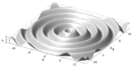
Figure 1: An example of the radially periodic axisymmetric potential, $V(r)=-\cos(2r)$.

Stationary axially symmetric states with chemical potential $\mu$ are looked for as solutions to Eq. (1) in the form of $u=e^{-i\mu t}U(r)$, with a real function $U$ obeying the equation

$$\mu U+\left(\frac{d^{2}}{dr^{2}}+\frac{1}{r}\frac{d}{dr}\right)U-V(r)U+\chi U^{3}=0.$$ (3)

For given potential $V(r)$, solutions to Eq. (3) form families parameterized by $\mu$ or, alternatively, by the norm,

$$N=2\pi\int_{0}^{\infty}\left(U(r)\right)^{2}rdr\equiv N=2\pi\int_{0}^{\infty}|u|^{2}rdr.$$ (4)

Solutions to stationary equation (3) with $\chi=+1$ (self-attraction) were obtained by means of a recently developed spectral-renormalization method for finding self-localized states of nonlinear-Schrödinger (NLS) type equations am . Independently, the same stationary solutions were also generated by dint of the well-known method which uses the integration of GPE (1) in imaginary time chiofalo . Stability of the solitary waves was then tested by adding small perturbations to them and integrating the GPE in real time. A stable perturbed soliton would shed off some radiation, which was absorbed at boundaries of the integration domain, and relax into a slightly different stationary form, corresponding to the smaller norm.

In the case of repulsion ($\chi=-1$), self-localized states were obtained by solving Eq. (1) in real time, with an absorber placed at the boundary of the integration domain. In that case, a localized waveform (e.g., Gaussian) with a suitable norm was chosen as the initial condition. In the course of the evolution, excess norm is radiated away with linear waves, which are absorbed at the boundary, and a self-localized state emerges (see an example in Fig. 4 below). It is obvious that solitons found this way are stable.

The above-mentioned radial lattices of the Bessel type can be naturally generated by a nondiffracting linear optical beam with the cylindrical symmetry (Bessel beams themselves are usually generated by means of axicoms) Durnin . On the other hand, the radial potential of the form $\cos(2kr)$ can be induced, as said above, by a cylindrical beam whose amplitude is modulated as $\cos(kr)$. The modulation can be provided by passing the cylindrical laser beam through a properly shaped plate PLA ; experiment . Unlike the Bessel beam, the one with the $\cos(kr)$ transverse modulation will suffer conical diffraction, but it is not a problem for BEC experiments, as a tight optical trap created in the transverse direction may readily contain a 2D pancake-shaped configuration of the condensate, of the thickness $\simeq 2$ $\mu$m layer . The diffraction of the paraxial beam, with waist diameter $D\sim 100$ $\mu$m, relevant to the experiment, on such a short propagation distance is completely negligible, as the respective diffraction length (alias Rayleigh range) is estimated to be $z_{\mathrm{diffr}}\sim D^{2}/\lambda\sim 10$ mm, where $\lambda\sim 1$ $\mu$m is the beam’s carrier wavelength.

III Solitons trapped at the center

III.1 Numerical solutions

It is known that a radial potential structure can easily trap a soliton in the central potential well kartashov . We start the consideration of the present model with solutions of this type. Typical examples of the solitonic shape in the model with self-attraction ($\chi=+1$) are displayed in Fig. 2. These solutions were obtained by means of both the above-mentioned spectral-renormalization method am and integration in imaginary time chiofalo .

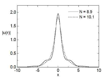
Figure 2: Axial cross sections of two stable solitons with equal chemical potentials, $\mu=-0.5$, trapped (in the model with self-attraction) at the center of the radial structure, $V(r)=\varepsilon\cos(2r)$, with $\varepsilon=1.5$ (in this case, the norm is $N=8.9$; solid line), and $\varepsilon=0.5$ ($N=10.1$, dashed line).

In the repulsive model ($\chi=-1$), numerical solutions were obtained, as said above, by solving Eq. (1) in real time, in the presence of the boundary absorber. An example of the relaxation of an initial Gaussian pulse into a soliton is given in Fig. 3. Full views of the typical stable solitons trapped at the center of the radial structure in the model with self-attraction and self-repulsion are displayed in Fig. 4.

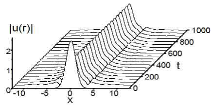
Figure 3: Formation of a self-trapped state (radial gap soliton) in repulsive BEC in the radial lattice with strength $\varepsilon=3$ (in the presence of absorbers at the boundary of the integration domain) from an initial Gaussian with norm $N=6\pi$. The norm of the eventually established state is $N=5.63$, i.e., $\approx 30\%$ of the initial value.

 

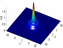
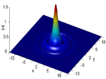
Figure 4: Left panel: The same localized state in the attractive BEC whose axial cross section is shown by the solid curve in Fig. 2 (with $N=8.9$, $\mu=-0.5$, and $\varepsilon=1.5$). Right panel: A localized state in the repulsive BEC, with $N=5.63$, $\mu=1.88$, amplitude $A=1.358$, and $\varepsilon=3$, which was generated as shown in Fig. 3.

As concerns the solitons in the repulsive model ($\chi=-1$), a typical example of which is displayed in the right panel of Fig. 4, they may be clearly classified as solitons of the gap type, since they exist solely due to the interplay of the lattice potential and self-defocusing nonlinearity. The ordinary setting that gives rise to gap solitons is quite similar, with the OL in the 1D, 2D or 3D Cartesian coordinates GS . Slowly decaying fringes, attached to the central core of the soliton and evident in the right panel of Fig. 4 (and absent in the ordinary soliton displayed in the left panel), is a characteristic feature of gap solitons. Thus, this self-trapped state may be naturally called a radial gap soliton.

III.2 Variational approximation

To describe a stationary soliton trapped in the central potential well in an analytical approximation, we adopt a Gaussian ansatz,

$$U(r)=A\exp\left(-\frac{r^{2}}{2a^{2}}\right).$$ (5)

Comparison with Fig. 2 shows that, in the model with attraction ($\chi=+1$), this ansatz is quite adequate for solitons with a larger norm, trapped in a relatively weak lattice, but it may be inaccurate as an approximation for solitons with smaller $N$ trapped in a stronger lattice.

The application of the variational approximation (VA) to stationary equation (3), with the help of the accordingly modified Lagrangian (2), is straightforward (cf. Refs. bms2003 ; bms2004 ; Estoril , where the same Gaussian ansatz was used to predict 2D solitons trapped in quasi-1D and square OLs). Thus we arrive at a set of VA-generated equations that relate the soliton’s size $a$ to its norm and chemical potential:

$$\frac{\chi N}{4\pi}=1-\frac{1}{2}\varepsilon a^{3}\frac{df}{da},\quad\mu=\varepsilon\left[a\frac{df}{da}+f(a)\right]-\frac{1}{a^{2}},$$ (6)

where $f(a)=1-\sqrt{\pi}ae^{-a^{2}}\mathrm{erfi}(a)$, $\mathrm{erfi}(a)\equiv\mathrm{erf}(ia)/i$, and $\mathrm{erf\ }$is the standard error function.

The analysis of dependence $\mu=\mu(N)$ following from Eq. (6) with $\chi=+1$ (self-focusing) predicts the existence of a family of solitons trapped at the center of the radial lattice, which are stable according to the Vakhitov-Kolokolov (VK) stability criterion VK ; berge , $d\mu/dN<0$, as shown in Fig. 5. Although the VK criterion is only necessary for the stability, as it ignores a possibility of oscillatory instability with complex eigenvalues, direct simulations of Eq. (1) confirm the stability of these solutions (see below).

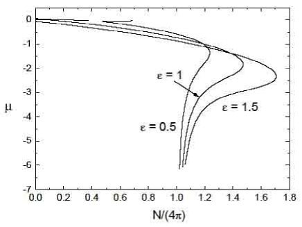
Figure 5: Dependences $\mu=\mu(N)$ following from variational equations (6), for the self-attraction case, $\chi=+1$. According to the VK criterion, $d\mu/dN<0$, stable solutions belong to upper branches of the curves.

Additional evidence for the existence of self-trapped localized states of BEC in the present model can be provided by a more general, time-dependent, version of the VA. To this end, we define a generalized ansatz [cf. Eq. (5)]

$$u(r,t)=A(t)\exp\left[-\frac{r^{2}}{2\left(a(t)\right)^{2}}+\frac{i}{2}b(t)r^{2}+i\phi(t)\right],$$ (7)

where $b\$is a real radial chirp. Applying the standard VA procedure malomed2 , one arrives at the following evolution equation for the width of the localized state,

$$\frac{d^{2}a}{dt^{2}}=\frac{4(1-\chi^{\prime})}{a^{3}}+2\varepsilon\left[2a+\sqrt{\pi}(1-2a^{2})e^{-a^{2}}\mathrm{erfi}(a)\right],$$ (8)

where an effective nonlinearity strength is

$$\chi^{\prime}\equiv\chi N/(4\pi),$$ (9)

and the amplitude is given by

$$A^{2}(t)=N/\left(\pi a^{2}(t)\right).$$ (10)

Equation (8) describes motion of a unit-mass particle with the coordinate $a(t)$ in an effective potential

$$U(a)=\frac{2(1-\chi^{\prime})}{a^{2}}-2\sqrt{\pi}\varepsilon ae^{-a^{2}}\mathrm{erfi}(a).$$ (11)

In Fig. 6 the effective potential (11) is depicted for different values of $\chi^{\prime}$, for the attractive and repulsive versions of the model.

 

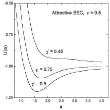
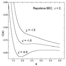
Figure 6: The variational potential, as given by Eq. (11) for different values of $\chi^{{}^{\prime}}=\chi N/(4\pi)$, at fixed strength $\varepsilon$ of the radial optical lattice.

Solitons in the attractive BEC ($\chi=+1$) exist when potential (11) possesses a local minimum. In particular, for $\varepsilon=0.5$ (see Fig. 6), the potential minimum exists provided that $\chi^{\prime}>0.45$. For the norm smaller than that corresponding to $\chi^{\prime}=0.45$ [see Eq. (9)], the self-attraction is too weak to form a soliton, and the matter-wave pulse spreads out through barriers of the radial potential. On the other hand, in the case of attraction, $\chi^{\prime}$ is also limited from above, by the collapse occurring at a critical value, $\chi_{\mathrm{cr}}^{\prime}=N_{\mathrm{cr}}/(4\pi)$. In the absence of the lattice ($\varepsilon=0$), a numerically exact critical norm is $N_{\mathrm{cr}}^{(0)}\simeq 11.7$ (it is equal to the norm of the Townes soliton) berge . For any $\varepsilon$, the VA predicts $\chi_{\mathrm{cr}}^{\prime}=1$, as the value of coefficient $\chi^{\prime}$ at which the first term in effective potential (11) vanishes. According to Eq. (9), this gives $N_{\mathrm{cr}}^{(\mathrm{var})}=4\pi$ Sweden .

Thus, the VA predicts a finite existence region for stable self-trapped localized states in the attractive BEC; for example, it is $0.45<\chi^{\prime}<1$ for $\varepsilon=0.5$. While the upper edge of this region is fixed at $N=N_{\mathrm{cr}}^{(\mathrm{var})}=4\pi$, numerical analysis of expression (11) demonstrates that the lower critical norm necessary for the existence of the self-trapped state almost linearly decreases with the increase of the OL strength $\varepsilon$. Numerically exact solution of the $\theta$-independent version of full GPE (1) demonstrates that, although the collapse sets in at a critical value of the norm which is slightly higher than $N_{\mathrm{cr}}^{(\mathrm{var})}=4\pi$, similar to the case of the 2D soliton stabilized by the quasi-1D or square OL bms2003 ; bms2004 ; Estoril , the dependence of $N_{\mathrm{cr}}$ on $\varepsilon$ is weak. The physical mechanism behind the rise of the collapse threshold in a trapping potential is that the confinement allows the soliton to increase the internal “quantum pressure”, generated by the dispersion term in GPE (1), which counteracts the nonlinear self-focusing of the wave packet.

Predictions of the VA for dynamical regimes can be compared to direct simulations in terms of the time dependence of the amplitude, $A(t)$, in a soliton which was excited by a sudden perturbation [the variational prediction for $A(t)$ is taken as per Eq. (10)]. To display an example, we take the stationary solution from Fig. 2, corresponding to $\varepsilon=0.5$ and $N=10.1$, and suddenly increase the lattice strength to $\varepsilon=0.75$. Comparison of the variational results with simulations of Eq. (1) is presented in Fig. 7. As observed, agreement for absolute values of the amplitude is, at best, qualitative, while the oscillation frequencies coincide much better.

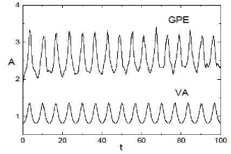
Figure 7: Comparison of a result of the variational approximation (“VA”) with direct simulations of Eq. (1) (“GPE”) with $\chi=+1$, in terms of the soliton’s amplitude as a function of time. Intrinsic vibrations of the soliton were triggered by sudden increase of the lattice strength from $\varepsilon=0.5$ to $\varepsilon=0.75$, for the self-trapped state with $N=10.1$ in Fig. 2.

In the case of the repulsive BEC ($\chi=-1$), the behavior is opposite, as seen in the right panel of Fig. 6. In this case, a larger norm for given OL strength $\varepsilon$ causes spreading of the localized state, because the self-defocusing nonlinearity overcomes the confining effect of the trapping potential. Simulations of Eq. (1) with $\chi=-1$ show that the wave packet sheds off excessive norm in the form of linear waves, which are absorbed at domain boundaries, and relaxes into a stable shape after the norm becomes adequate. For example, at $\varepsilon=2$ stable localized states in the repulsive BEC exist at $|\chi^{\prime}|$ ${}_{\sim}^{<}~{}1$ [i.e., the norm is limited to values $N$ ${}_{\sim}^{<}~{}4\pi$, see Eq. (9)].

IV Ring-shaped solitons

IV.1 Analytical approach

The most essential property of radially periodic potentials is that localized states can self-trap not only in the central potential well, but also in remote circular troughs kartashov . If the trough’s curvature is not significant, these localized states resemble 2D solitons in the quasi-1D OL reported in Ref. bms2004 . Here, we aim to derive an asymptotic 1D equation for patterns trapped in a circular trough, and obtain its relevant solutions. To this end, we adopt the following ansatz for the solution,

$$\psi(r,\theta,t)=\sqrt{2}A(y,t)\mathrm{sech}\left(x/\rho\right),$$ (12)

where $y\equiv r_{0}\theta$ is the coordinate running along the circumference of radius $r_{0}$, $A(y,t)$ is a slowly varying complex amplitude, and the transverse variable is $x\equiv r-\pi m$, with $r_{0}\equiv\pi m$ being a radial potential minimum in a vicinity of which the ring-shaped pattern is trapped. Assuming $m$ to be large enough, we consider the annular pattern placed in a remote circular trough, which may be treated as a quasi-rectilinear potential trap, with negligible curvature. Obviously, the latter condition amounts to $\rho\ll r_{0}$ [recall $\rho$ is the radial size in ansatz (12)].

Neglecting the curvature in Eq. (1), we rewrite it as a 2D equation with $x$ and $y$ treated as local Cartesian coordinates,

$$i\frac{\partial\psi}{\partial t}+\frac{\partial^{2}\psi}{\partial x^{2}}+\frac{\partial^{2}\psi}{\partial y^{2}}+\chi\left|\psi\right|^{2}\psi-\varepsilon\cos\left(2x\right)\psi=0.$$ (13)

The next step is to reduce Eq. (13) to an effectively 1D equation along azimuthal direction $y$. To this end, we note that Eq. (13) corresponds to the Lagrangian [cf. Eq. (2)]

$$L=\int\int dxdy \left[\frac{i}{2}\left(\psi_{t}\psi^{\ast}-\psi\psi_{t}^{\ast}\right)-\left(\left|\psi_{x}\right|^{2}+\left|\psi_{y}\right|^{2}\right)\right.$$ (14)

$$\left.+\frac{1}{2}\chi\left|\psi\right|^{4}-\varepsilon\cos(2x)\left|\psi\right|^{2}\right].$$

In this Lagrangian, we substitute ansatz (12) and integrate the resulting expression in transverse direction $x$. After a straightforward calculation, this yields an effective (averaged) Lagrangian,

$$L_{\mathrm{eff}} = 2\int_{-\infty}^{+\infty}dy\left[i\rho\left(A_{t}A^{\ast}-AA_{t}^{\ast}\right)-2\rho\left|A_{y}\right|^{2}-2I\frac{\rho_{y}^{2}}{\rho}|A|^{2}\right.$$ (15)

$$\left.-\frac{2\left|A\right|^{2}}{3\rho}+\frac{4}{3}\chi\rho\left|A\right|^{4}-\frac{2\pi\varepsilon\rho^{2}\left|A\right|^{2}}{\sinh\left(\pi\rho\right)}\right],$$

where $I\equiv\int_{0}^{+\infty}\left(\mathrm{sech}^{2}x-\mathrm{sech}^{4}x\right)x^{2}dx\approx 0.61$.

The application of the standard variational procedure to averaged Lagrangian (15) gives rise to a cumbersome system of coupled equations for the complex amplitude $A(y,t)$ and real width $\rho(y,t)$. The equations strongly simply if we assume that $A$ and $\rho$ are slowly varying functions of $y$, which, in particular, corresponds to long-wave perturbations that account for the onset of the modulational instability (MI), see below. In particular, in the attractive model ($\chi=+1$) one may first adopt the lowest-order approximation, completely neglecting the $y$-dependence and assumes time-independent $|A|$ and $\rho$, which gives rise to a result previously known from the application of the VA to the NLS equation in 1D with potential $\cos(2kx)$ Wang :

$$|A|=\sqrt{\frac{1}{\rho^{2}}+\frac{3}{2}\varepsilon\pi\rho\left[\pi\rho\frac{\cosh(\pi\rho)}{\sinh^{2}(\pi\rho)}-\frac{1}{\sinh\left(\pi\rho\right)}\right]}.$$ (16)

This relation is cumbersome too, but straightforward analysis demonstrates that it takes a very simple form, $|A|=1/\rho$, when $\varepsilon$ is both small and large [in the latter case, scaling $|A|\sim\rho^{-1}\sim\varepsilon^{-1/2}$ is assumed, to lend the last three term in the Lagrangian density in Eq. (15) the same order of magnitude].

To obtain a closed-form Lagrangian for the amplitude field $A(y,t)$ in the attractive model, one should express $\rho$ in Eq. (15) in terms of $\left|A\right|$, using relation (16). This will lead, in the general case, to a messy result; however, the above-mentioned simplest approximation, $\rho=1/\left|A\right|$, which replaces Eq. (16), yields a tractable expression,

$$L_{\mathrm{eff}} = 2\int_{-\infty}^{+\infty}dy\left\{i\left(A_{t}\sqrt{\frac{A^{\ast}}{A}}-A_{t}^{\ast}\sqrt{\frac{A}{A^{\ast}}}\right)+\frac{4}{3}\left|A\right|^{3}\right.$$ (17)

$$\left.-\frac{I}{2}\left[\frac{\left(A_{y}^{\ast}\right)^{2}}{A^{\ast}}\sqrt{\frac{A}{A^{\ast}}}+\frac{A_{y}^{2}}{A}\sqrt{\frac{A^{\ast}}{A}}\right]\right.$$

$$\left.-\left(2+I\right)\frac{\left|A_{y}\right|^{2}}{\left|A\right|}-2\varepsilon|A|\right\}$$

[the last term in the Lagrangian density should be dropped if $\varepsilon$ is small; if $\varepsilon$ is large, the term is obtained within the framework of the above scaling, that assumes small $\rho$, hence $\sinh(\pi\rho)\approx\pi\rho$]. Finally, the action functional, $S=\int L_{\mathrm{eff}}dt$, as defined by Lagrangian (17), gives rise to the Euler-Lagrange equation, $\delta S/\delta A^{\ast}=0$, in the following form:

$$i\tilde{A}_{t}+(2+I)\tilde{A}_{yy}-\left(1+\frac{3I}{4}\right)\frac{\tilde{A}_{y}^{2}}{\tilde{A}}+I\left[\frac{\tilde{A}}{\tilde{A}^{\ast}}\tilde{A}_{yy}^{\ast}\right.$$

$$\left.+\frac{\left|\tilde{A}_{y}\right|^{2}}{2\tilde{A}^{\ast}}-\frac{3}{4}\frac{\left(\tilde{A}_{y}^{\ast}\right)^{2}\tilde{A}}{\left(\tilde{A}^{\ast}\right)^{2}}\right]+2\left|\tilde{A}\right|^{2}\tilde{A}=0,$$ (18)

where $\tilde{A}(y,t)\equiv A(y,t)e^{-i\varepsilon t}$ [this transformation eliminates a linear term in the equation generated by the last term in Lagrangian (17)].

Formally setting $I=0$ in Eq. (18) recovers an equation known as a model for the propagation of surface waves on a plasma layer with a sharp boundary Gradov . A class of nonpolynomial generalized NLS equations similar to Eq. (18), and some of their fundamental solutions, such as single-soliton ones, were introduced in Ref. Lennart (see also Ref. Nattermann ).

Stationary solutions to Eq. (18) with chemical potential $\mu$ are looked for in the ordinary form, $\tilde{A}(y,t)=\allowbreak e^{-i\mu t}B(y)$, with $B(y)$ satisfying equation $(1+I)\left[2B^{\prime\prime}-(B^{\prime})^{2}/B\right]+2B^{3}+\mu B=0$, where $B^{\prime}\equiv dB/dy$. This equation has its Hamiltonian,

$$H=(2/3)B^{3}+\mu B+(1+I)(B^{\prime})^{2}/B,$$ (19)

Setting $H=0$, one obtains a family of soliton solutions, for any $\mu<0$:

$$B_{\mathrm{sol}}(y)=\sqrt{-\frac{3\mu}{2}}\mathrm{sech}\left(\sqrt{-\frac{\mu}{1+I}}y\right).$$ (20)

For $H<0$ and $\mu<0$, a family of periodic cnoidal-wave solutions is obtained in the form

$$B_{\mathrm{cn}}(y)=\frac{B_{0}B_{1}}{B_{1}+\left(B_{0}-B_{1}\right)\mathrm{cn}^{2}\left(\sqrt{\frac{B_{0}\left(B_{1}+\left|B_{2}\right|\right)}{6\left(1+I\right)}}y,q\right)},$$ (21)

where $\mathrm{cn}(z,q)$ is the Jacobi’s elliptic cosine, with modulus

$$q=\sqrt{\frac{B_{0}-B_{1}}{B_{0}}\cdot\frac{\left|B_{2}\right|}{B_{1}+\left|B_{2}\right|}}<1,$$ (22)

and $B_{2}<0<B_{1}<B_{0}$ are three roots of equation $(2/3)B^{3}+\mu B-H=0$ [it is obtained by setting $B^{\prime}=0$ in Eq. (19)]. Solutions (21) exist, for given $\mu<0$, in a region of $0\leq-H\leq\left(\sqrt{2}/3\right)|\mu|^{3/2}$; as said above, the limit of $H=0$ corresponds to soliton (20), and the opposite limit, $H=-\left(\sqrt{2}/3\right)|\mu|^{3/2}$, corresponds to a uniform CW (continuous-wave) solution, with

$$B_{0}=B_{1}\equiv B(y)=\sqrt{|\mu|/2},~{}B_{2}=-\sqrt{2|\mu|}.$$ (23)

Cnoidal solutions on the ring of radius $r_{0}$ must satisfy the corresponding periodic boundary conditions (b.c.), $\tilde{A}(y,t)=\tilde{A}(y+2\pi r_{0},t)$ (for the ordinary 1D NLS equations with repulsion and attraction, analytical solutions satisfying the periodic b.c. are collected in Refs. Carr-repulsive and Carr-attractive , respectively). Accordingly, parameter $H$ in solutions (21), (22) is not continuous, but rather takes discrete values selected by matching the b.c. to the periodicity of $\mathrm{cn}^{2}$,

$$\frac{\pi r_{0}}{n}=\sqrt{\frac{6\left(1+I\right)}{B_{0}\left(B_{1}+\left|B_{2}\right|\right)}}K(q),$$ (24)

where $K$ is the complete elliptic integral, and $n$ is an arbitrary integer.

Note that Eq. (18) features the Galilean invariance: if $\tilde{A}(y,t)$ is a solution, then its counterpart in the form of a solution moving at an arbitrary velocity $v$ is

$$\tilde{A}_{c}(y,t)=\tilde{A}(y-vt)\exp\left(\frac{i}{4}vy-\frac{i}{2}v^{2}t\right),$$ (25)

hence one can boost solitons (20) and cnoidal waves (21) to a (formally) arbitrary velocity by means of transformation (25). In fact, the velocity is not arbitrary because the factor $\exp\left(ivy/4\right)$ also must satisfy the periodic b.c., which leads to a quantization condition, $v=4n/r_{0}$, with $n=0,\pm 1,\pm 2,\,...$ .

IV.2 Modulational instability of the uniform ring soliton in the model with attraction

In the model with attraction ($\chi=+1$), the existence of uniform ring-shaped solitons trapped in annular troughs of large radii is obvious, while a nontrivial issue is a possibility of finding a stability region for such solutions. In terms of Eq. (18), the ring soliton is represented by a CW (continuous-wave) solution with a constant amplitude $B_{0}$, which was mentioned above as a limit case of the cnoidal solution family, with $\mu=-2B_{0}^{2}$.

It is well known that, while all CW solutions of NLS-like equations with attraction are modulationally unstable [including nonpolynomial equations similar to Eq. (18) Lennart ], periodic b.c. may stabilize them if the CW amplitude is smaller than a certain critical value. This argument suggests a possibility to find a stability region for the uniform ring solitons in the present model with attraction.

A standard analysis of the MI assumes a perturbation of the CW solution,

$$\tilde{A}(y,t)=\left[B_{0}+B_{1}(y,t)\right]\exp\left(2iB_{0}^{2}t+i\chi_{1}(y,t)\right),$$

with infinitesimal amplitude and phase perturbations $B_{1}$ and $\chi_{1}$. Eigenmodes of the perturbations may be looked for assuming that they are proportional to $\exp\left(ipy+\gamma t\right)$, where $p$ is an arbitrary real wavenumber, and $\gamma$ is the corresponding instability growth rate. Straightforward calculations demonstrate that the CW solution to Eq. (18) is subject to the MI under the condition

$$p^{2}\left[2B_{0}^{2}-(1+I)p^{2}\right]>0.$$ (26)

In the annular system that we are dealing with, $p$ is subjected to the geometric quantization, the same way as above, i.e., $p=n/r_{0}$ with integer $n$. Therefore, condition (26) with lowest $|n|=1$ is not satisfied, making the CW solution  modulationally stable, under the condition

$$2B_{0}^{2}r_{0}^{2}\leq 1+I.$$ (27)

In a final form, this stability condition may be expressed in terms of the full norm of the axisymmetric ring soliton. Substituting ansatz (12) in Eq. (4), and making use of the assumptions adopted above, one obtains $N\approx 8\pi r_{0}\rho B_{0}^{2}$. Further, substituting here the above approximation, $\rho=1/B_{0}$, yields

$$N=8\pi r_{0}B_{0}.$$ (28)

With regard to this relation, stability condition (27) amounts to a limitation on $N$:

$$N<N_{\mathrm{thr}}=4\sqrt{2(1+I)}\pi\approx 22.55\text{.}$$ (29)

(note that this result does not contain any parameter).

A natural way to look at these stability conditions is to consider a situation with gradually increasing $N$ (or $B_{0}$). The azimuthally uniform ring solution will loose its stability when the amplitude (or norm) attains the critical value defined by Eq. (27) [or by Eq. (29)]. One may expect that the onset of the MI gives rise to a bifurcation, which creates stable azimuthally modulated solutions, with a modulation depth scaling as $\sqrt{N-N_{\mathrm{thr}}}$ for $0<\left(N-N_{\mathrm{thr}}\right)/N_{\mathrm{thr}}\ll 1$. Alternatively, one may fix the CW amplitude, $B_{0}$, and gradually increase the trough’s radius $r_{0}$; the loss of the CW stability and emergence of the modulated solutions should occur when $r_{0}$ attains a critical value following from Eq. (27),

$$\left(r_{0}\right)_{\mathrm{cr}}=\sqrt{(1+I)/2}B_{0}^{-1}.$$ (30)

In fact, the modulated states generated by the MI onset should be nothing else but the stationary cnoidal wave (21), (22). Indeed, with regard to Eq. (23) and the fact that $K(0)=\pi/2$, it follows form matching condition (24) that, with the increase of $r_{0}$ for fixed $B_{0}$, the cnoidal-wave solution appears, with an infinitely small modulation depth, at $r_{0}=\left(r_{0}\right)_{\mathrm{cr}}$, where the critical value $\left(r_{0}\right)_{\mathrm{cr}}$ is precisely the same as defined by the onset of the MI [i.e., given by Eq. (30)].

A defect of the above approximate analysis is that, with regard to relation $A_{0}=1/\rho$, stability condition (29) may be cast in the form of $\rho/r_{0}>\sqrt{2/(1+I)}\approx\allowbreak 1.\allowbreak 1$, which does not comply with the underlying low-curvature assumption, $\rho_{0}\ll r_{0}$. This fact makes the existence of modulationally stable ring-shaped solitons in the present model with attraction doubtful. In direct simulations of Eq. (1) with $\chi=+1$, we were unable to find modulationally stable annular uniform nonlinear states. In this connection, it is relevant to recall that the linear limit of Eq. (1) with potential $V(r)=\varepsilon\cos(2r)$ does not allow any stationary solution localized in the radial direction, therefore the weak nonlinearity is essential in stabilizing the axisymmetric rings.

Note that localized ring-shaped states may be possible in the linear limit of the Bessel-lattice models considered in Refs. kartashov and repulsion , with potentials $-\varepsilon J_{0}\left(kr\right)$ and $-\varepsilon J_{1}^{2}\left(kr\right)$, respectively; however, the azimuthal (in)stability of such states was not studied in the presence of attraction. On the other hand, stable annular patterns (both static ones and persistent ring-shaped breathers) were recently found in an attractive model with a single circular trough, which was created not by the linear potential, but rather by modulation of the nonlinear coefficient in the radial direction HS . In that model, annular states may only be stable if the annulus is wide enough, with the ratio of its outer and inner radii exceeding $0.47$. Vorticity-carrying rings were found to be unstable in the same setting.

IV.3 Gap Soliton nature of ring shaped states

In this section we investigate the gap soliton nature and the band structure associated with ring shaped states in terms of the following 2D GPE

$$i\psi_{t}=-\Delta_{r}\psi+\varepsilon\cos(2r)\psi+\chi|\psi|^{2}\psi$$ (31)

where $\Delta_{r}$ denotes the spherical 2D laplacian: $\Delta_{r}=\frac{\partial^{2}}{\partial r^{2}}+\frac{2}{r}\frac{\partial}{\partial r}-\frac{\hat{l}^{2}}{r^{2}}$, with $\hat{l}^{2}=-\frac{\partial^{2}}{\partial\varphi^{2}}$ the squared 2D angular momentum. This equation corresponds to the $\theta\rightarrow\frac{\pi}{2}$ limit ($u(r,\pi/2,\varphi)\rightarrow\psi(r,\varphi)$) of the spherically symmetric 3D GPE, with $(r,\theta,\varphi)$ denoting spherical coordinates. Notice that apart for the factor of two in front of the term $\frac{1}{r}\frac{\partial}{\partial r}$, due to spherical rather than cylindrical symmetry, Eq. (31) is the same as Eq. (1). From a physical point of view Eq. (31) is appropriate to describe a condensate trapped in the outer part of the conical region created by a cylindrical beam of light passed through a very short focal distance lens. In the following we shall refer to this setting as the ”pizza” geometry since, in contrast with the pancake geometry, the thickness of the condensate in the axial direction is not uniform and reduces to zero as $r\rightarrow 0$. This geometry could be implemented by combining a cylindrical beam creating the radial lattice with a blue-detuned conical beam (the pizza-shaper)

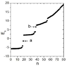
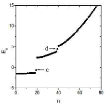
Figure 8: Left Panel: Energy levels of Eq. (34) with $\chi=-1$, $l=10$ and $\varepsilon=10$. Right panel: The same as in the left panel for the repulsive case $\chi=1$ with $l=2$ and $\varepsilon=-4$.

launched in the opposite direction. Notice that at large radial distances (i.e. in the outer part of the pizza) the differences between pancake and pizza geometry become negligible especially if the thickness of the border is very small compared to the radius. Ring shaped states of Eq. (31) located in potential wells far from the center are expected, therefore, to be qualitatively similar to the ones of the pancake setting Eq. (1).

In the following we look for ring gap solitons of Eq. (31) in the form of stationary states $\psi(r,\varphi,t)$ of the form

$$\psi(r,\varphi,t)=\phi(r)e^{-i\mu t}e^{il\varphi}.$$ (32)

By substituting Eq. (32) into Eq.(31) we obtain the following equation for the radial function $\phi(r)$

$$\phi_{rr}+\frac{2}{r}\phi_{r}+(\mu-\varepsilon\cos(2r))\phi-(\chi|\phi|^{2}+\frac{l^{2}}{r^{2}})\phi=0,$$ (33)

where $l$ are integer numbers which allow to satisfy the periodic boundary condition in $\varphi$: $\psi(r,\varphi+2\pi,t)=\psi(r,\varphi,t)$. Equation (33) can be mapped into a 1D eigenvalue problem by means of the transformation $\phi(r)=\frac{\xi(r)}{r}$ leading to the following reduced radial equation

$$\xi_{rr}+[E-\varepsilon\cos(2r)-\frac{l^{2}+\chi|\xi|^{2}}{r^{2}}]\xi=0$$ (34)

which has the form of a 1D Schrödinger equation with periodic potential and nonlinear effective centrifugal barrier: $(l^{2}+\chi|\xi|^{2})/r^{2}$ (here $E\equiv\mu$). For sufficiently large distances $r\gg 1$ and fixed angular momentum and nonlinearity, this equation reduces to the Mathieu equation with the well known band gap structure. The part of the spectrum associated to excitations localized nearby the origin, however, is expected to be strongly influenced by the centrifugal barrier which at short distances enhances the nonlinearity and favors the formation of localized states.

To investigate the band structure and the gap solitons of Eq. (34) we use a self-consistent method developed in Ref. ms05 . The gap solitons obtained with the self-consistent method will then be used as initial conditions for time propagation of the radial 2D GPE in Eq. (1).

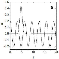
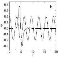
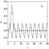
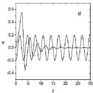
Figure 9: Panels a,b. Attractive radial gap solitons (thick lines) trapped in circular troughs of the potential at $r=1.5\pi$ and corresponding to the energy levels $a,b$ of the left panel of Fig. 8, respectively. Panels c,d. Repulsive radial gap solitons (thick lines) trapped in circular troughs of the potential at $r=1.5\pi$ and corresponding to the energy levels $c,d$ of the right panel of Fig. 8, respectively. The thin lines corresponds to the radial potential $\varepsilon\cos(2r)$ scaled by a factor $50$ in the left panel and by a factor $20$ in the right panel, for graphical convenience.

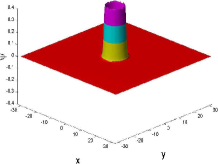
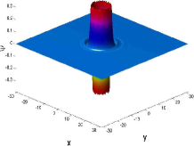
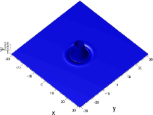
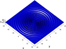
Figure 10: Top panels. 3D view of the gap solitons corresponding to the bound states a (left panel) and b (right panel) of Fig. 8. Bottom panels. 3D view of the gap solitons corresponding to the bound states c (left panel) and d (right panel) of Fig. 8.

As a result we show the existence of radially symmetric gap solitons which correspond to the ring shaped states discussed before.

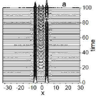
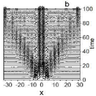
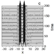
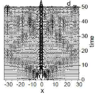
Figure 11: Time evolution ($y=0$) section of $|\psi|^{2}$ obtained from Eq. (1) by taking as initial conditions the localized states depicted in panels a-d of Fig. 9. The norm of the attractive states in panels $a,b$ are $4.85$, $4.81$, respectively, and correspond to bound states a,b, of Fig. 8. Repulsive states in panels $c,d$ have norm $11.47$ and $9.17$, respectively, and correspond to the bound states c,d, of Fig. 8. Parameters are the same as in corresponding panels of Fig. 8.

In Fig. 8 we depict the lower energy part of the spectrum obtained from Eq. (34) in the case of attractive and repulsive interactions. We see in both cases the existence of a series of discrete levels located in the gaps between the bands which correspond to radially symmetric localized states. The wave functions of the energy levels labeled a-d in Fig. 8 are shown in Fig. 9.

The symmetries of these localized states is similar to the ones of intrinsic localized modes of nonlinear lattices and gap solitons of continuous 1D GPE with a periodic potential. Adopting the same terminology introduced for these cases we shall refer to them as the onsite symmetric and the onsite asymmetric ring gap solitons. A 3D plot of these states is reported in Fig. 10 (notice that the asymmetric state gives two rings of matter located in the same trough of the potential in the attractive case and many ring oscillations in the repulsive case ). The stability of these gap solitons has been checked by time propagation under the 2D GPE in Eq. (1). The results are reported in Fig. 11 for the $y=0$ section of of $|\psi(x,y,t)|^{2}$ as a function of time. We see that for the attractive case the gap solitons are always unstable, the onsite symmetric state becomes modulationally unstable at $t\approx 80$ while the asymmetric state decays into a state localized in the center and a series of ring solitons which expand trough the lattice keeping the same symmetry as the initial state. For the repulsive case we see that while the asymmetric state in the second band gap (panel d) is unstable, the onsite symmetric ring gap soliton in the first band gap is quite stable under time evolution. The stability of the onsite symmetric repulsive ring gap solitons and the modulational instability of the repulsive ones has been found also for other parameter values and seems to be a general property of the model. The existence of other types of ring gap solitons (which resemble intersite symmetric and asymmetric intrinsic localized modes of nonlinear lattices) is also possible but they look even more unstable under time evolution than the onsite asymmetric ones for both attractive and repulsive cases. In the following section we shall investigate onsite symmetric gap soliton states in more details.

IV.4 Numerical investigation of ring-shaped states

Generic examples of a ring-shaped soliton in the attractive model, and its counterpart in the repulsive one, found from direct solution of GPE (1) in, respectively, imaginary and real time, are displayed in Fig. 12 (in the latter case, real-time simulations were run with absorbers set at $r=8\pi$ and $r=0$). The latter example represents radial gap solitons with the core trapped in a remote circular trough (cf. the right panel in Fig. 4 that shows a radial gap soliton with the core trapped in the center). The fact that the soliton belongs to the gap type is clearly attested to by conspicuous inner and outer radial fringes attached to the core (the fringes are absent in the ordinary soliton in the left panel of the figure).

 

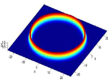
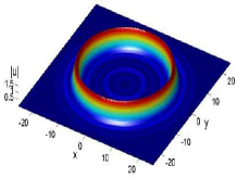
Figure 12: Left panel: An unstable ring-shaped soliton in the attractive model with $\varepsilon=2$, trapped in a circular trough at $r_{0}=6\pi$. The amplitude of this soliton is $1.8$, and its chemical potential and norm are $\mu=-2.3$ and $N\simeq 420$. Note that analytical approximation (28) yields, in this case, $N\simeq 426$, which is very close to the numerically found value, and its modulational instability is definitely predicted by Eq. (29). Right panel: A stable ring-shaped soliton (actually, it is a radial gap soliton) in the repulsive model with $\varepsilon=3$, trapped at $r_{0}=5\pi$. In the latter case, $N=344.3$ and $\mu=0.78$.

The evolution of the unstable axisymmetric ring from Fig. 12 (left panel), and outcome of the evolution are displayed in Fig. 13. It is observed that the system tends to form a stationary necklace-like pattern composed of six peaks towering above the remaining quasi-uniform background.

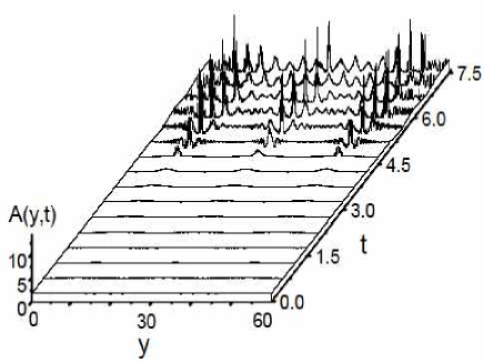
(a)

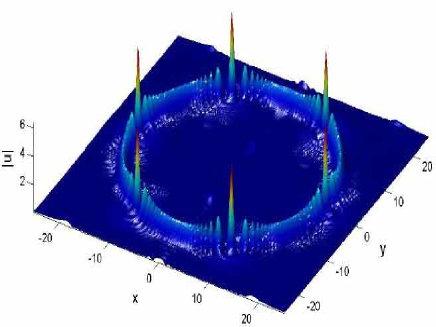
(b)

Figure 13: (a) Development of the modulational instability of the axisymmetric state in Fig. 12 (left panel), triggered by a small azimuthal perturbation, $\delta u=0.02\,\cos(6\phi)\,\exp\left(-(r-r_{0})^{2}/2\right)$. The evolution is shown in terms of the amplitude, $|A(y,t)|$, taken along circumference $y=r_{0}\theta$, with $r_{0}=6\pi$, $\theta$ running from $0$ to $\pi$ (due to the symmetry, only half of the circle is shown). (b) The field profile formed by $t=5$, demonstrating the emergence of a regular necklace-shaped pattern.

In the repulsive model, a stable ring (i.e., the radial gap soliton) may additionally carry, on its crests, pairs of dark solitons. An example of such a pattern is displayed in Fig. 14 (it resembles the dipole-mode ring soliton recently found in the model with repulsion and Bessel lattice in Ref. Ricardo ).

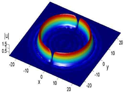
Figure 14: An example of a stable configuration formed by two dark solitons created on top of a ring-shaped soliton in the repulsive model with $\varepsilon=3$, trapped at $r_{0}=5\pi$. This state has norm $N=330.6$ and chemical potential $\mu=0.80$.

Stable static rings with a density modulation in the azimuthal direction, corresponding to analytical solutions (21) for the cnoidal waves, have been found too in the attractive model. A typical example of such a pattern is displayed in Fig. 15; in fact, it was generated as an outcome of the evolution of an unstable axisymmetric ring with the same norm.

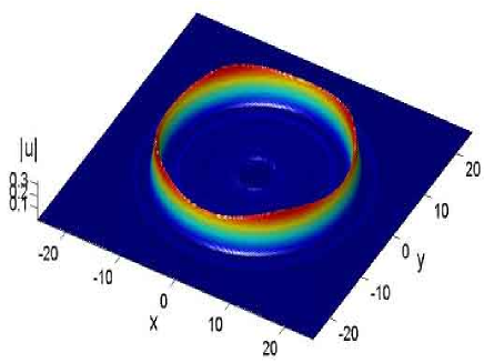
Figure 15: A stable ring-shaped soliton featuring weak azimuthal modulation, in the model with attraction and strong radial lattice ($\varepsilon=10$). The solution’s norm and chemical potential are $N=7.2$ and $\mu=-5.7$.

Increase of the norm leads to a transition from weakly modulated stable patterns to deeply modulated ones. An example of such a stable configuration, generated from four Gaussian pulses, with the phase shifts $\pi$ between them, by integration of Eq. (1) in imaginary time, is displayed in Fig. 16 (note that the total norm of this pattern exceeds that corresponding to Fig. 15 by a factor of $\simeq 3.5$).

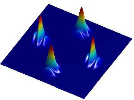
Figure 16: A stable set of four solitons in the attractive model, trapped in a circular trough with $r_{0}=5\pi$ and $\varepsilon=2$. The norm of each soliton is $N=2\pi$, with the phase difference $\pi$ between adjacent ones. The lattice is embedded in an integration domain of size $16\pi\times 16\pi$.

V Rotational dynamics and collisions between solitons

V.1 Stability of rotary solitons

Strongly localized solitary waves of the attractive BEC, self-trapped in a large-radius annular potential channel, like those shown in Fig. 16, can freely move along in the channel. If set in motion with a sufficiently small velocity, the soliton can circulate in the channel indefinitely long, preserving its integrity, as shown in Fig. 17.

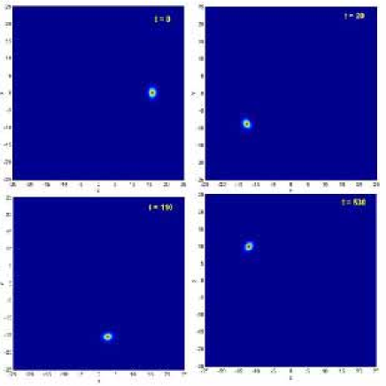
Figure 17: A stable soliton in the attractive model, with norm $N=9.42$, trapped in the circular trough at $r_{0}=5\pi$, was set in motion in the clockwise direction with velocity $v=1$. As illustrated by the sequence of snapshots, the circular motion in the trough continues indefinitely long without any visible loss.

However, when the circulation speed is too large, the centrifugal force acting on the soliton can cause the matter to tunnel into adjacent radial troughs. The loss of the norm (number of atoms) caused by the centrifugal tunneling eventually brings the soliton’s norm below the threshold value necessary for its existence, which leads to disintegration of the soliton, see Fig. 18.

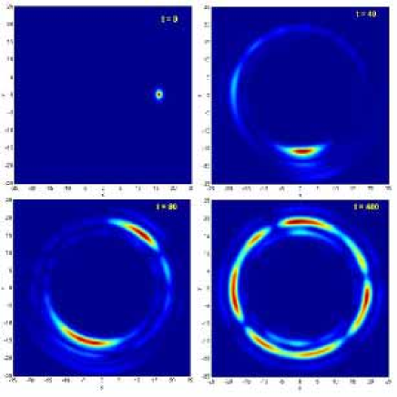
Figure 18: If the same soliton as in Fig. 17 (with initial norm $N=9.42$) is set in motion with a greater velocity, $v=3$, the centrifugal force gives rise to the underbarrier leakage of atoms into the outer circular troughs. As illustrated by the sequence of snapshots, the decaying soliton cannot preserve its shape. The norm remaining within the given radial channel at $t=400$ is $N_{\mathrm{final}}\simeq 0.5$, i.e., $\simeq 5\%$ of the initial value.

If the lattice is weak, and the soliton is strongly self-trapped (with a sufficiently large norm), the centrifugal force can also drive it away from the center, across the lattice. In that case (not shown here), the soliton also suffers the radiation loss, and eventually disintegrates.

V.2 Collisions between solitons

The present model offers unique possibilities for exploring interactions and collisions between matter-wave solitons, as the dynamics in circular channels is free of external perturbations, which are always present in previously reported settings (in the form of the weak longitudinal trap intended to keep the solitons within a finite spatial domain). The same advantage is offered by setups with the toroidal trap torus-experiment ; torus-theory . However, sideline (tangential) collisions, which are possible between solitons moving in adjacent potential troughs of the radial lattice, have no counterparts in the toroidal traps.

In head-on collisions of solitons in the attractive model (in the same circular channel), two competing processes play major roles. The first is the nonlinear self-focusing, which may give rise to intrinsic collapse of a large-norm “lump” temporarily formed by the colliding solitons, and the other is the interference due to coherence of the matter-wave solitons bms2004 ; Estoril . The interference pattern, featuring alternating regions of high and low density, can suppress the collapse. The predominance of either mechanism depends on the time of interaction. If it is small (in the case of large collision speed), solitons can pass trough each other without collapse (although with conspicuous loss, see below, hence the collision cannot be termed quasi-elastic), even if their total norm exceeds the collapse threshold. On the contrary, slow collisions lead to the onset of collapse. These two possible scenarios of the head-on collisions between in-phase (mutually attracting) solitons are shown in Figs. 19 and 20.

Figure 19 presents an example of a relatively fast collision. At the moment of the full overlap between the solitons, $t=4.3$, the interference fringes are evident, and are also seen in the cross section along the circumference of the channel (lower right panel). Although the total norm of the colliding solitons is overcritical ($N_{\mathrm{tot}}=14.9$), and the collision time ($\Delta t\simeq 0.5$) is larger than the collapse time (which is estimated as $t_{\mathrm{collapse}}\sim 1/N_{\mathrm{tot}}$) , the solitons separate without collapse. Nevertheless, the collision is essentially inelastic, the loss being additionally enhanced by the matter leakage under the action of the centrifugal force. On the other hand, Fig. 20 shows that the solitons colliding at a sufficiently small velocity merge together and indeed blow up due to the collapse.

 

 

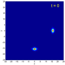
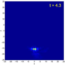
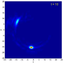
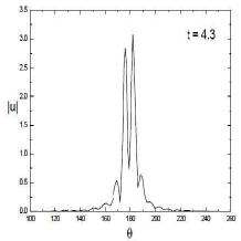
Figure 19: Collision between two solitons with individual norms $N=2.5\pi$ and zero phase difference, in the circular trough at $r_{0}=5\pi$. One of the solitons is set in motion (at $x=5\pi,y=0$) at $t=0$ with speed $v=3$ in the clockwise direction, while the second one (at $x=0,y=-5\pi$) stays quiescent. The norm remaining within the given circular channel at $t=10$ is $N_{\mathrm{final}}=12.75$. The soliton which was originally at rest loses less norm than the moving one.

 

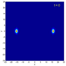
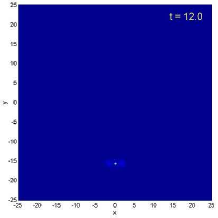
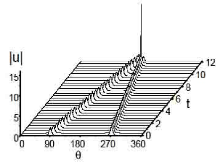
Figure 20: The head-on collision of two in-phase solitons in the attractive model, when both of them were set in motion with relatively small velocities, $v=\pm 1$, in one circular channel ($r_{0}=5\pi$), ends up with collapse. Upper panels: density plots at $t=0$ and the moment of collapse ($t=12$). Lower panel: the evolution of the density profiles in the cross section along the circumference of the potential trough. As in Fig. 19, the initial norm of each soliton is $N=2.5\pi$.

Two $\pi$ out-of-phase solitons colliding in the same potential trough bounce from each other due to repulsion between them. Then, repeated bouncing collisions are observed, which is similar to the dynamics in the Bessel lattice kartashov , as well as in a quasi-1D OL, equipped with a weak longitudinal trap bms2004 . However, in contrast to those works, we have observed that many collisions in the circular trough gradually wash out the phase coherence between the solitons. As a result, the solitons cease to repel each other, and a clear interference pattern disappears. Eventually, the originally repelling solitons merge together, shedding the excessive norm away, as shown in Fig. 21. The intrinsic collapse does not occur in this case, as the loss makes the norm of the finally established single soliton smaller than the critical value at the collapse threshold.

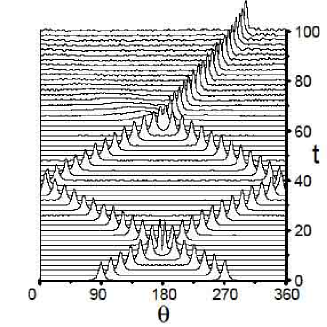
Figure 21: Collision of two solitons with the same parameters as in Fig. 20, but the phase difference of $\pi$ between them. Solitons bounce at $\theta=180^{\mathrm{o}}$ and $\theta=0^{\mathrm{o}}$. Finally, the solitons merge into a single one, without collapse.

Collisions of matter-wave solitons in the attractive BEC is accompanied by strong exchange of matter between them. The present setting makes it possible to investigate related phenomena for solitons moving in adjacent channels of the radial potential, and thus colliding tangentially. The result is that two in-phase solitons are unstable against the flow of matter in this setting, and tend to merge (a similar trend was observed in the model with a quasi-1D lattice in Ref. bms2004 ). Nevertheless, the solitons may avoid collapse and separate, if the collision time is small due to a large relative velocity, as shown in Fig. 22 .

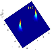
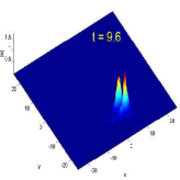
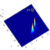
Figure 22: A sequence of snapshots for the collision between solitons with individual norms $N=2\pi$, moving at velocities $v=\pm 1$ in adjacent troughs (at $r_{0}=5\pi$ and $r_{0}=4\pi$) of the radial lattice with $\varepsilon=2$. The solitons survive the collision, and remain localized, although the collision is inelastic, giving rise to radiation loss.

On the other hand, if the solitons are loosely bound (i.e. their norms are small and/or the radial lattice is weak), the slow lateral collision gives rise to merger of the solitons into one, excessive norm being shed off with linear waves, as demonstrated in Fig. 23.

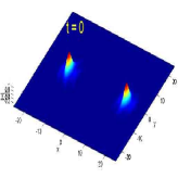
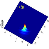
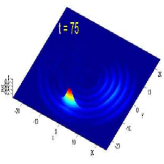
Figure 23: The same as in Fig. 15, but for solitons with smaller norms, $N=1.7\pi$, launched to move at velocities $v=\pm 0.2$.

VI Conclusions

In this work, we have proposed a new setting to explore two-dimensional (2D) localized states in self-attractive and repulsive BECs, in the form of a periodic radial optical lattice. A crucial difference from previously studied 2D models with Bessel lattices is the fact that no localized state may exist in the linear limit of the present model, hence all solitary states in it are “true solitons”, impossible without the nonlinearity. Besides the BEC, the model may also apply to spatial solitons (beams) in photonic crystal fibers with a circular intrinsic structure.

The existence of such objects was demonstrated by means of different variants of the variational approximation, and in direct numerical simulations. We have investigated the localized states trapped in the central potential well and in remote circular potential troughs. In both cases, a new species, namely, stable radial gap solitons, have been identified in the model with self-repulsion (in addition, the radial gap soliton trapped in a circular trough can carry stable pairs of dark solitons on its crest). In remote troughs, we have investigated ring-shaped patterns delocalized in the azimuthal direction, as well as strongly localized azimuthal solitons (including moving ones). In the attractive model, solutions of both types are described by an effective 1D equation supplemented by the periodic boundary conditions (it is a nonpolynomial NLS equation with the coordinate running along the circumference). In particular, a finite threshold of the azimuthal modulational instability (MI) of axisymmetric ring-shaped states was predicted, and exact cnoidal-wave solutions, generated by the MI-induced bifurcation were found in the framework of the 1D equation. Azimuthal solitons were also found as solutions to the same equation. The existence of stable azimuthally uniform and weakly modulated ring-shaped states was corroborated by direct simulations.

Dynamics of completely localized solitons circulating in the annular potential troughs was investigated in the attractive model by means of direct simulations. In particular, the solitons with sufficiently small velocities remain stable indefinitely long, while high velocities give rise to leakage of matter into the adjacent (more remote) trough under the action of the centrifugal force, which eventually destroys the soliton. Collisions between solitary waves running in the same or adjacent circular channels were investigated too. Head-on collisions of the in-phase solitons in one trough lead to the collapse; $\pi$-out of phase solitons bounce from each other many times, but gradually loose their mutual coherence, and eventually merge into a single soliton without collapsing, shedding off excess norm. In-phase solitons colliding in adjacent channels may also merge into a single soliton.

References

- (1) J. Denschlag, J. E. Simsarian, D. L. Feder, C. W. Clark, L. A. Collins, J. Cubizolles, L. Deng, E. W. Hagley, K. Helmerson, W. P. Reinhardt, S. L. Rolston, B. I. Schneider, and W. D. Phillips, Science 287, 97 (2000); S. Burger, K. Bongs, S. Dettmer, W. Ertmer, K. Sengstock, A. Sanpera, G. V. Shlyapnikov, and M. Lewenstein, Phys. Rev. Lett. 83, 5198 (1999);
- (2) L. Khaykovich, F. Schreck, G. Ferrari, T. Bourdel, J. Cubizolles, L. D. Carr, Y. Castin, and C. Salomon, Science 296, 1290 (2002).
- (3) K. E. Strecker, G. B. Partridge, A. G. Truscott, and R. G. Hulet, Nature 417, 150 (2002)
- (4) S. L. Cornish, S. T. Thompson, and C. E. Wieman, cond-mat/0601664.
- (5) N. G. Parker, A. M. Martin, S. L. Cornish and C. S. Adams, cond-mat/0603059.
- (6) B. Eiermann, Th. Anker, M. Albiez, M. Taglieber, P. Treutlein, K. -P. Marzlin, and M. K. Oberthaler, Phys. Rev. Lett. 92, 230401 (2004).
- (7) V. A. Brazhnyi and V. V. Konotop, Mod. Phys. Lett. B 18, 627 (2004); O. Morsch and M. Oberthaler, Rev. Mod. Phys. 78, 179 (2006).
- (8) B. A. Malomed, D. Mihalache, F. Wise, and L. Torner, J. Opt. B: Quantum Semiclass. Opt. 7, R53 (2005).
- (9) B. B. Baizakov, B. A. Malomed, and M. Salerno, Phys. Rev. A 70, 053613 (2004).
- (10) D. Mihalache, D. Mazilu, F. Lederer, Y. V. Kartashov, L.-C. Crasovan, and L. Torner, Phys. Rev. E 70, 055603(R) (2004).
- (11) M. Trippenbach, M. Matuszewski, and B. A. Malomed, Europhys. Lett. 70, 8 (2005); M. Matuszewski, E. Infeld, B. A. Malomed, and M. Trippenbach, Phys. Rev. Lett. 95, 050403 (2005).
- (12) B. A. Malomed, Soliton Management in Periodic Systems (Springer: New York, 2006).
- (13) Y. V. Kartashov, V. A. Vysloukh, and L. Torner, Phys. Rev. Lett. 93, 093904 (2004).
- (14) Y. V. Kartashov, V. A. Vysloukh, and L. Torner, Phys. Rev. Lett. 94, 043902 (2005).
- (15) Y. V. Kartashov, R. Carretero-Gonzalez, B. A. Malomed, V. A. Vysloukh, and L. Torner, Opt. Exp.13, 10703(2005).
- (16) N. Moiseyev, L. D. Carr, B. A. Malomed, and Y. B. Band, J. Phys. B 37, L193 (2004).
- (17) L. D. Carr, M. J. Holland, and B. A. Malomed, J. Phys. B 38, 3217 (2005).
- (18) Q. E. Hoq, P. G. Kevrekidis, D. J. Frantzeskakis, and B. A. Malomed, Phys. Lett. A 341, 145 (2005).
- (19) X. Wang, Z. Chen, and P. G. Kevrekidis, Phys. Rev. Lett. 96, 083904 (2006).
- (20) R. Fischer, D. N. Neshev, S. Lopez-Aguayo, A. S. Desyatnikov, A. A. Sukhorukov, W. Krolikowski, and Y. S. Kivshar, Opt. Exp. 14, 2825 (2006).
- (21) D. Mihalache, D. Mazilu, F. Lederer, B. A. Malomed, Y. V. Kartashov, L.-C. Crasovan, and L. Torner, Phys. Rev. Lett. 95, 023902 (2005).
- (22) A. S. Desyatnikov, A. A. Sukhorukov, and Y. S. Kivshar, Phys. Rev. Lett. 95, 203904 (2005).
- (23) S. Gupta, K. W. Murch, K. L. Moore, T. P. Purdy, and D. M. Stamper-Kurn, Phys. Rev. Lett. 95,143201 (2005).
- (24) A. Parola, L. Salasnich, R. Rota, and L. Reatto, Phys. Rev. A 72, 063612 (2005); R. Kanamoto, H. Saito, and M. Ueda, Phys. Rev. A 73, 033611 (2006).
- (25) E. Lidorikis, M. Soljaćić, M. Ibanescu, Y. Fink, and J. D. Joannopoulos, Opt. Lett. 29, 851(2004).
- (26) Z. H. Musslimani and J. Yang, J. Opt. Soc. Am. B 21, 973 (2004); M. J. Ablowitz, and Z. H. Musslimani, Opt. Lett. 30, 2140 (2005).
- (27) M. L. Chiofalo, S. Succi, and P. Tosi, Phys. Rev. E 62, 7438 (2000).
- (28) B. B. Baizakov, V. V. Konotop and M. Salerno, J. Phys. B: At. Mol. Opt. Phys. 35, 5105 (2002); E. A. Ostrovskaya and Y. S. Kivshar, Phys. Rev. Lett. 90, 160407 (2003).
- (29) J. Durnin, J. J. Miceli, and J. H. Eberly, Phys. Rev. Lett. 58, 1499 (1987).
- (30) A. Görlitz, J. M. Vogels, A. E. Leanhardt, C. Raman, T. L. Gustavson, J. R. Abo-Shaeer, A. P. Chikkatur, S. Gupta, S. Inouye, T. Rosenband, and W. Ketterle, Phys. Rev. Lett. 87, 130402 (2001).
- (31) B. A. Malomed, Progr. Optics 43, 69 (E. Wolf, editor: North Holland, Amsterdam, 2002).
- (32) B. B. Baizakov, B. A. Malomed and M. Salerno, Europhys. Lett., 63, 642 (2003).
- (33) B. B. Baizakov, M. Salerno, and B. A. Malomed, in: Nonlinear Waves: Classical and Quantum Aspects, ed. by F. Kh. Abdullaev and V. V. Konotop, p. 61 (Kluwer Academic Publishers: Dordrecht, 2004); also available at http://rsphy2.anu.edu.au/~asd124/Baizakov_2004_61_Nonlinear Waves.pdf.
- (34) M. G. Vakhitov and A. A. Kolokolov, Radiophys. Quant. Electr. 16, 783 (1973).
- (35) Mario Salerno, Laser Physics 15, 620 (2005).
- (36) L. Bergé, Phys. Rep. 303, 260 (1998).
- (37) M. Desaix, D. Anderson, and M. Lisak, J. Opt. Soc. Am. B 8, 2082 (1991).
- (38) B. A. Malomed, Z. H. Wang, P. L. Chu, and G. D. Peng, J. Opt. Soc. Am. B 16, 1197 (1999).
- (39) L. Stenflo and O. M. Gradov, IEEE Trans. Plasma Sci. PS-14, 554 (1986); L. Stenflo, J. Phys. A 21, L499 (1988).
- (40) B. A. Malomed and L. Stenflo, J. Phys. A 24, L1149 (1991).
- (41) P. Nattermann, Phys. Scripta 50, 609 (1994).
- (42) L. D. Carr, C. W. Clark, and W. P. Reinhardt, Phys. Rev. A 62, 063610 (2000).
- (43) L. D. Carr, C. W. Clark, and W. P. Reinhardt, Phys. Rev. A 62, 063611 (2000).
- (44) H. Sakaguchi and B. A. Malomed, Phys. Rev. E 73, 026601 (2006).