Magnetoresistance of a quantum dot with spin-active interfaces

Abstract

We study the zero-bias magnetoresistance ($\mathrm{MR}$) of an interacting quantum dot connected to two ferromagnetic leads and capacitively coupled to a gate voltage source $V_{g}$. We investigate the effects of the spin-activity of the contacts between the dot and the leads by introducing an effective exchange field in an Anderson model. This spin-activity makes easier negative $\mathrm{MR}$ effects, and can even lead to a giant $\mathrm{MR}$ effect with a sign tunable with $V_{g}$. Assuming a twofold orbital degeneracy, our approach allows to interpret in an interacting picture the $\mathrm{MR}(V_{g})$ measured by S. Sahoo et al. [Nature Phys. 2, 99 (2005)] in single wall carbon nanotubes with ferromagnetic contacts. If this experiment is repeated on a larger $V_{g}-$range, we expect that the $\mathrm{MR}(V_{g})$ oscillations are not regular like in the presently available data, due to Coulomb interactions.

I Introduction

The quantum mechanical spin degree of freedom is now widely exploited to control current transport in electronic devices. For instance, the readout of magnetic hard disks is based on the spin-valve effect, i.e. the tunability of a conductance through the relative orientation of some ferromagnetic polarizations Prinz . However, realizing spin injection in mesoscopic conductors would allow to implement further functionalities, like e.g. a gate control of the spin valve effect Datta ; Schapers . Importantly, electronic interaction effects can occur in mesoscopic structures, due to the electronic confinement. This raises the fundamental question of the interplay between spin-dependent transport and electronic interactions.

Upon scattering on the interface between a ferromagnet (F) and a non-magnetic material, electrons with spin parallel or antiparallel to the magnetization of F can pick up different phase shifts, because they are affected by different scattering potentials. This Spin-Dependence of Interfacial Phase Shifts (SDIPS) can modify significantly the behavior of mesoscopic circuits. First, when a mesoscopic conductor is connected to several F leads with non collinear polarizations, the SDIPS produces an interfacial precession of spins which can modify current transport in the device FNF ; Luttinger ; Wetzels ; Ciuti ; ReviewBraatas . Secondly, in collinear configurations, precession effects are not relevant, but the SDIPS can modify mesoscopic coherence effects. For instance, in superconducting/ferromagnetic hybrid circuits, the SDIPS introduces a phase shift between electron and holes correlated by Andreev reflection SF . References Tokuyasu, and SF2005, have identified signatures of this effect in the experiments of Refs. Tedrow, and Takis, , respectively. In principle, normal systems in collinear configurations can also be affected by the SDIPS. Indeed, from Ref. wire2005, , the SDIPS should produce a spin-splitting of the resonant states in a ballistic interactionless wire contacted with collinearly polarized ferromagnetic leads. However, this has not been confirmed experimentally yet comment .

Figure 1: Mesoscopic element M connected to ferromagnetic leads $L$ and $R$. The magnetic polarizations $\vec{p}_{L}$ and $\vec{p}_{R}$ of leads $L$ and $R$ can be parallel (configuration P) or antiparallel (configuration AP). The element M is capacitively coupled to a gate voltage source $V_{g}$.

Recently, Ref. Sahoo, has reported current measurements in a single wall carbon nanotube (SWNT) connected to two ferromagnetic leads with collinear polarizations. The asymmetries observed in the magnetoresistance ($\mathrm{MR}$) of the SWNT versus gate voltage are strikingly similar to those predicted by Ref. wire2005, for an interactionless wire subject to the SDIPSquestion . However, the SWNT of Ref. Sahoo, showed a quantum dot behavior with strong Coulomb Blockade effects, as demonstrated in a great number of experiments with non-magnetic leads (see e.g. expCB ; Sapmaz ). Therefore, one important question is how interaction effects modify the scheme proposed by Ref. wire2005, . The problem of the effects of interactions on the transport properties of a central region connected to ferromagnetic contacts has already been considered in various regimes, like e.g. the Coulomb blockade regimeWetzels ; CB ; Braun ; Weymann , the Kondo regimeKondo ; Martinek , the Luttinger liquid regimeLuttinger ; Luttinger2 and the marginal Fermi liquid regimeMFL . This article develops an approach suitable for the limit of Ref. Sahoo, and studies, for the first time, the effect of the SDIPS on a quantum dot. We consider a quantum dot coupled to metallic leads through spin-active interfaces. We use an Anderson model to study the $\mathrm{MR}$ of the circuit above the Kondo temperature, but beyond the sequential tunneling limit. The SDIPS is taken into account through an effective spin-splitting of the dot energy levels. This splitting makes easier negative $\mathrm{MR}$ effects. When it is strong enough, it can even lead to a giant $\mathrm{MR}$ with a sign oscillating with the dot gate voltage $V_{g}$, similarly to what has been found in the non-interacting case. In the non-interacting case, assuming that the properties of the contact are constant with energy and that the SDIPS is too weak to split the conductance peaks, one finds that the $\mathrm{MR}(V_{g})$ pattern is similar for all conductance peaks. In contrast, the effect of the SDIPS depends on the occupation of the dot in the interacting case. This is in apparent contradiction with the data of Ref. Sahoo, because, in the $V_{g}-$range presented in this Ref., the $\mathrm{MR}(V_{g})$ oscillations are regular. Using a two-orbitals model, which takes into account the $K-K^{\prime}$ orbital degeneracy commonly observed for SWNTs (see e.g. Refs. Liang, ; Jarillo, ; Sapmaz, ; Moriyama, ; Babic, ; Babic2, ), one can solve this discrepancy. In this framework, we expect non-regular $\mathrm{MR}(V_{g})$ oscillations if the experiment is repeated on a larger $V_{g}-$range.

This article is organized as follows: we start with summarizing the results found for the non-interacting case in section II.1. Then we introduce a model for the interacting case in section II.2. Section III addresses the case of a one-orbital quantum dot circuit, and section IV the case of a two-degenerate-orbitals quantum dot circuit. Finally section V concludes.

II Model

We consider a mesoscopic element M connected to ferromagnetic leads $L$ and $R$ (Fig. 1). The chemical potential of M can be shifted by $e\alpha V_{g}$ using the gate voltage $V_{g}$, with $\alpha$ the ratio between the gate capacitance and the total capacitance of $M$. The magnetic polarizations $\vec{p}_{L}$ and $\vec{p}_{R}$ of leads $L$ and $R$ can be parallel (configuration $c=P$) or antiparallel (configuration $c=$ $AP$).

II.1 Non-interacting case

Before introducing the interacting model investigated in this article, it is useful to reconsider the results obtained by Ref. wire2005, for the case in which M is a non-interacting single-channel ballistic wire of length $L$. In a scattering approachBlanter , the conductance of the circuit depends on the transmission probability $T_{l}^{c,\sigma}$ for electrons with spin $\sigma\in\{\uparrow,\downarrow\}$ through contact $l\in\{L,R\}$, and on the reflection phase $\varphi_{l}^{c,\sigma}$ for electrons with spin $\sigma$ coming from the wire towards contact $l$. The index $c=P[AP]$ denotes the parallel [antiparallel] leads configuration. A spin dependence of $\varphi_{l}^{c,\sigma}$ can occur due to the magnetic properties of the contact materials used to engineer lead $l$. Due to size quantization, the conductance $G^{c}(V_{g})$ of the circuit in configuration $c$ presents Fabry-Perot like resonances for $E_{d,\sigma}^{c}\sim 0$, with $E_{d,\sigma}^{c}=(2\pi d-\varphi_{L}^{c,\sigma}-\varphi_{R}^{c,\sigma})(2\pi N_{F}^{M})^{-1}-e\alpha V_{g}-E_{F}^{M}$ a resonant energy, $d\in\mathbb{Z}$, $E_{F}^{M}$ the wire Fermi energy, $N_{F}^{M}$ the density of orbitals states at the Fermi level in the wire and $\overline{\sigma}$ the spin direction opposite to $\sigma$ (we have used $e\alpha V_{g}\ll E_{F}^{M}$). From this Eq., in configuration $c$, the SDIPS produces a spin-splitting

$$g\mu_{B}h_{SDIPS}^{c}=E_{d,\downarrow}^{c}-E_{d,\uparrow}^{c}=\sum_{l\in\{L,R\}}\frac{\varphi_{l}^{c,\uparrow}-\varphi_{l}^{c,\downarrow}}{\pi N_{F}^{M}}$$ (1)

of the resonant energies. When the effective field $h_{SDIPS}^{c}$ is strong enough to produce a spin-splitting of the conductance peaks, the circuit can display a giant $\mathrm{MR}$ effect with a sign oscillating with $V_{g}$, due to the strong shift of the conductance peaks from the $P$ to the $AP$ configurations. In the opposite case, $\mathrm{MR}$ remains smaller, but the SDIPS can still be detected through characteristic asymmetries in the oscillations of $\mathrm{MR}$ versus $V_{g}$ (see Fig. 2-right of Ref. wire2005, ). Importantly, assuming that $T_{l}^{c,\sigma}$ and $\varphi_{l}^{c,\sigma}$ are constant with $V_{g}$, one has $G^{c}(V_{g})=G^{c}(V_{g}+[2/e\alpha N_{F}^{M}])$ . This implies that when $h_{SDIPS}^{c}$ is not strong enough to produce a spin-splitting of the conductance peaks, the $\mathrm{MR}(V_{g})$ pattern is similar for all the peaks displayed by $G^{P}(V_{g})$.

II.2 Interacting case

We now assume the presence of strong Coulomb interactions inside M, such that we have a quantum dot connected to ferromagnetic leads. Such a system can be realized for instance by using granular filmsgranular , nanoparticlesnanoparticles , carbon nanotubesSahoo ; tubes , or $C_{60}$ moleculesmolecules . In the non-interacting case of section II.1, we have considered that the spin-dependent confinement potential felt by electrons causes the SDIPS, which leads to the spin-splitting of the resonant states. In the interacting case, the scattering approach is not suitable anymore. However, the energy of the quasi-bound single particle states in quantum dot M can depend on spin due to the spin-dependent confinement potential. On this ground, we adopt the effective Anderson hamiltonian

$$H=H_{dot}+H_{leads}+H_{c}$$ (2)

with

$$H_{dot} =\sum\limits_{d,\sigma}\xi_{d\sigma}c_{d\sigma}^{\dagger}c_{d\sigma}+\sum\limits_{\begin{subarray}{c}d,d^{\prime},\sigma,\sigma^{\prime}\\ (d,\sigma)\neq(d^{\prime},\sigma^{\prime})\end{subarray}}\frac{U}{2}n_{d\sigma}n_{d^{\prime}\sigma^{\prime}}$$

$$H_{leads} =\sum\limits_{k,\sigma}\xi_{k\sigma}c_{k\sigma}^{\dagger}c_{k\sigma}$$

$$H_{c} =\sum\limits_{d,k,\sigma}\left(t_{d\sigma}^{k}c_{d\sigma}^{\dagger}c_{k\sigma}+(t_{d\sigma}^{k})^{\ast}c_{k\sigma}^{\dagger}c_{d\sigma}\right)$$

Here, $\xi_{d\sigma}$ refers to the energy of the dot orbital state $d$ for spin $\sigma$, $\xi_{k\sigma}$ to the energy of lead state $k$ for spin $\sigma$ and $t_{d\sigma}^{k}$ is an hoping matrix element (we assume that the spin $\sigma$ is preserved upon tunneling like in section II.1). The index $k$ runs over the electronic states of lead $L$ and $R$. Coulomb interactions are taken into account through the term in $U=e^{2}/C_{\Sigma}$, with $n_{d\sigma}=c_{d\sigma}^{\dagger}c_{d\sigma}$ and $C_{\Sigma}$ the total capacitance of the quantum dot M.  By construction of the model (see above), for $U=0$, each orbital level $\xi_{d\sigma}$ corresponds to a resonant level $E_{d\sigma}^{c}$ of section II.1, with $\xi_{d\downarrow}-\xi_{d\uparrow}=g\mu_{B}h_{SDIPS}^{c}$. We can therefore regard the effective Zeeman splitting $h_{SDIPS}^{c}$ in model (2) as a generalization of the SDIPS concept to the interacting caseexplanationWetzels . The specificity of this effective field, with respect to an ordinary external field, is that it depends on the configuration $c$ of the ferromagnetic electrodes. For instance, in the case of symmetric ferromagnetic contacts, symmetry considerations lead to $h_{SDIPS}^{P}\neq 0$ and $h_{SDIPS}^{AP}=0$.

In the following, we calculate the zero-bias conductance of the circuit using Meir2

$$\frac{h}{e^{2}}\frac{G^{c}}{2} =$$ (3)

$$\sum\limits_{d,\sigma}\int_{-\infty}^{+\infty}d\omega\frac{\partial f(\hbar\omega)}{\partial\hbar\omega}\frac{\Gamma_{d\sigma}^{L}(\hbar\omega)\Gamma_{d\sigma}^{R}(\hbar\omega)}{\Gamma_{d\sigma}^{L}(\hbar\omega)+\Gamma_{d\sigma}^{R}(\hbar\omega)}\operatorname{Im}[G_{d\sigma}(\omega)]\text{ .}$$

The above equation involves the retarded Green’s function $G_{d\sigma}(\omega)=\int_{-\infty}^{+\infty}\widetilde{G}_{d\sigma}(t)e^{i\omega t}dt$ with $\widetilde{G}_{d\sigma}(t)=-i\theta(t)\left\langle\left\{c_{d\sigma}(t),c_{d\sigma}^{\dagger}(0)\right\}\right\rangle$. We also use the Fermi distribution $f(\xi)=(1+\exp[\xi])^{-1}$ and the tunnel transition rates $\Gamma_{d\sigma}^{l}(\xi)=\sum\limits_{k}2\pi\left|t_{d\sigma}^{k}\right|^{2}\delta(\xi=\xi_{k\sigma})$ with $l\in\{L,R\}$. Note that $G_{d\sigma}$, $\xi_{d\sigma}$ and $\Gamma_{d\sigma}^{l}$ depend on the configuration $c\in\{P,AP\}$ considered but for simplicity we omit the index $c$ in those quantities. We want to study current transport in the limit studied in Ref. Sahoo, , i.e. the width of conductance peaks displayed by the circuit is determined not only by temperature but also by the tunnel rates ($\Gamma_{d\sigma}^{L}+\Gamma_{d\sigma}^{R}$ $\sim 2k_{B}T$). This requires to go beyond the sequential tunneling description, i.e. to take into account high-order quantum tunneling processes. For this purpose, we will calculate $G_{d\sigma}$ using the equation of motion (E.O.M.) techniqueMeir , which is valid for temperatures larger than the Kondo temperature $T_{K}$ of the systemnote SA .

III Single level quantum dot

For simplicity, we first take into account a single orbital level $d$ of the dot. We follow the lines of Ref. Meir, . The E.O.M. technique leads to

$$\frac{G_{d\sigma}(\omega)}{\hbar}=\frac{1-\left\langle n_{d\overline{\sigma}}\right\rangle}{\hbar\omega-\xi_{d\sigma}-\Sigma_{\sigma}^{S}}+\frac{\left\langle n_{d\overline{\sigma}}\right\rangle}{\hbar\omega-\xi_{d\sigma}-\Sigma_{\sigma}^{D}}$$ (4)

with

$$\left\langle n_{d\sigma}\right\rangle=-\int_{-\infty}^{+\infty}\frac{d\omega}{\pi}f(\hbar\omega)\operatorname{Im}[G_{\sigma}^{d}(\omega)]$$ (5)

the average occupation of orbital $d$ by electrons with spin $\sigma$. We define

$$\Sigma_{\sigma}^{S}=\Sigma_{d\sigma}^{0}-U\Sigma_{d\sigma,d\overline{\sigma}}^{1,1}[\hbar\omega-\xi_{d\sigma}-U-\Sigma_{d\sigma}^{0}-\Sigma_{d\sigma,d\overline{\sigma}}^{3,1}]^{-1}\,,$$ (6)

$$\Sigma_{\sigma}^{D}=U+\Sigma_{d\sigma}^{0}+U\Sigma_{d\sigma,d\overline{\sigma}}^{2,1}[\hbar\omega-\xi_{d\sigma}-\Sigma_{\sigma}^{0}-\Sigma_{d\sigma,d\overline{\sigma}}^{3,1}]^{-1}\,,$$ (7)

$$\Sigma_{d\sigma}^{0}=\sum\limits_{k}\left|t_{d\sigma}^{k}\right|^{2}\left(\hbar\omega-\xi_{k\sigma}+i0^{+}\right)^{-1}$$ (8)

and, for $i\in\{1,2,3\}$,

$$\Sigma_{d\sigma,d^{\prime}\sigma^{\prime}}^{i,n}=\sum\limits_{k}\frac{\mu_{i}(\xi_{k\sigma^{\prime}})\left|t_{k\sigma^{\prime}}^{d^{\prime}}\right|^{2}}{\hbar\omega-\xi_{d\sigma}+\xi_{d^{\prime}\sigma^{\prime}}-\xi_{k\sigma^{\prime}}+i0^{+}}\\ \mbox{}+\sum_{k}\frac{\mu_{i}(\xi_{k\sigma^{\prime}})\left|t_{k\sigma^{\prime}}^{d^{\prime}}\right|^{2}}{\hbar\omega-\xi_{d\sigma}-\xi_{d^{\prime}\sigma^{\prime}}-nU+\xi_{k\sigma^{\prime}}+i0^{+}}\,.$$ (9)

Here, one has $\mu_{1}(\xi)=f(\xi)$, $\mu_{2}(\xi)=1-f(\xi)$ and $\mu_{3}=1$ (We anticipate on the next paragraphs by defining $\Sigma_{d\sigma,d^{\prime}\sigma^{\prime}}^{i,n}$ for $n\in\mathbb{N}$ and an arbitrary dot state $d^{\prime}\sigma^{\prime}\neq d\sigma$, but only $n=1$ and $d^{\prime}\sigma^{\prime}=d\overline{\sigma}$ are needed for the present one-orbital case). We assume that the coupling to the leads is energy independent (broad band approximation), which gives e.g. $\Sigma_{d\sigma}^{0}=-i(\Gamma_{d\sigma}^{L}+\Gamma_{d\sigma}^{R})/2$. The term $\Sigma_{d\sigma}^{0}$, which is due to the tunneling of electrons with spin $\sigma$, already occurred in the non-interacting caseRelModel .

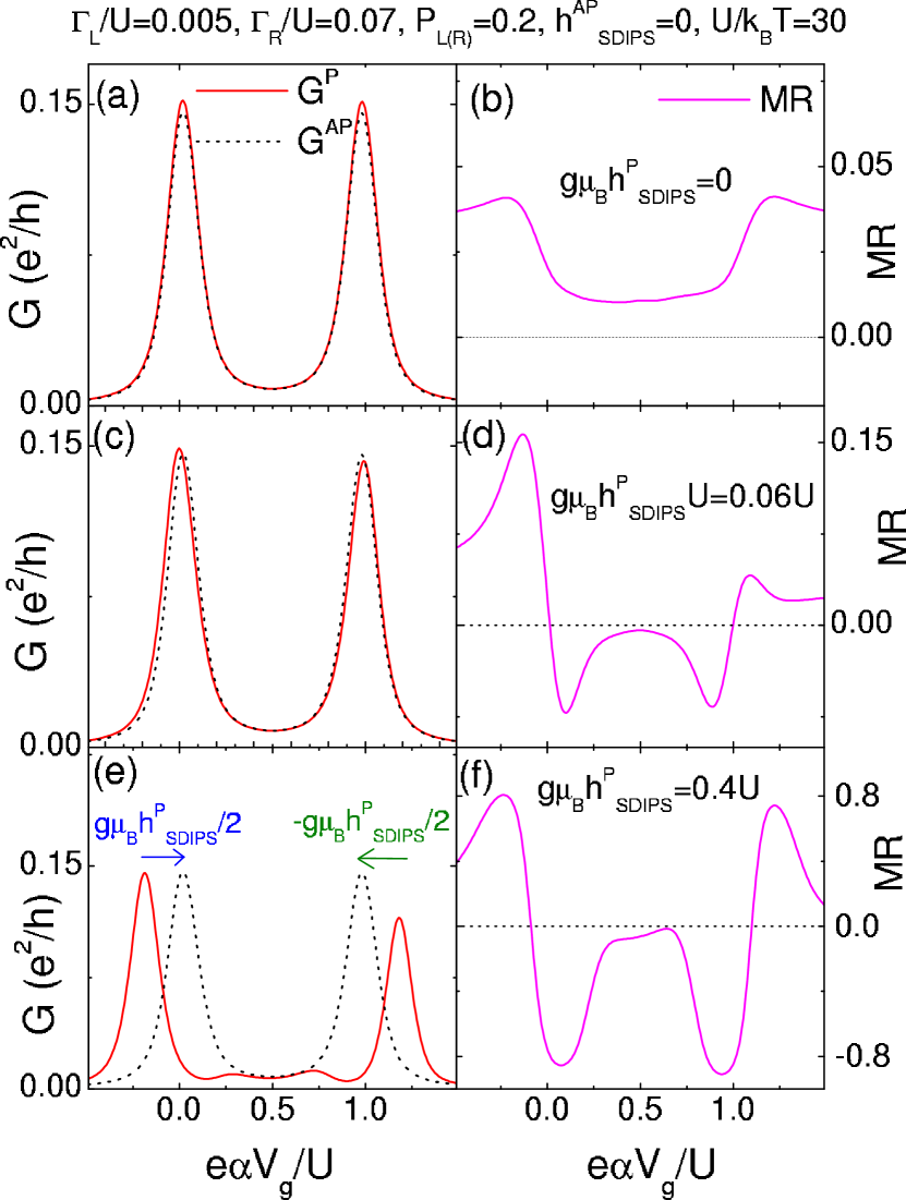
Figure 2: Panels a, c and e: Conductance $G^{P}$ in the parallel configuration (red full lines) and conductance $G^{AP}$ in the antiparallel configuration (black dotted lines) as a function of the gate voltage $V_{g}$, for the circuit shown in Fig. 1, with M a 1-orbital quantum dot. We have used $\Gamma_{L}=0.005U$, $\Gamma_{R}=0.07U$, $P_{L(R)}=0.2$, $U/k_{B}T=30$ and $h_{SDIPS}^{AP}=0$. Panels b, d, and f: Magnetoresistance $\mathrm{MR}=(G^{P}-G^{AP})/(G^{P}+G^{AP})$ (pink curves) corresponding to the left conductance plots. The results are shown for $g\mu_{B}h_{SDIPS}^{P}=0$ (panels a and b), $g\mu_{B}h_{SDIPS}^{P}=0.06U$ (panels c and d) and $g\mu_{B}h_{SDIPS}^{P}=0.4U$ (panels e and f).

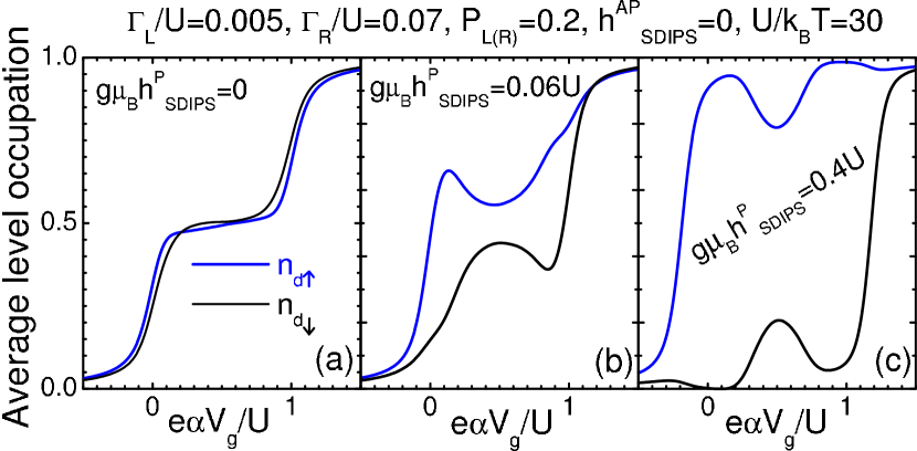
Figure 3: Average occupations $\left\langle n_{d\uparrow}\right\rangle$ (blue lines) and $\left\langle n_{d\downarrow}\right\rangle$ (black lines) of level $d$ by spins $\uparrow$ and $\downarrow$ as a function of $V_{g}$, for the 1-orbital quantum dot circuit of Fig. 1. The results are shown for the same parameters as in Fig. 2 and lead polarizations in the parallel configuration ($c=P$), with $h_{SDIPS}^{P}=0$ (panel a), $g\mu_{B}h_{SDIPS}^{P}=0.06U$, (panel b) and $g\mu_{BSDIPS}^{P}=0.4U$ (panel c). For $h_{SDIPS}^{P}=0$, $\left\langle n_{d\uparrow}\right\rangle$ and $\left\langle n_{d\downarrow}\right\rangle$ remain very close, simply showing two steps corresponding to the two conductances peaks visible in Fig. 2-a. In the case of a finite $h_{SDIPS}^{P}$, $\left\langle n_{d\uparrow}\right\rangle$ rises more strongly than $\left\langle n_{d\downarrow}\right\rangle$ at the first conductance peak, revealing that current transport is due in majority to $\uparrow$ spins for this first peak. Then, $\left\langle n_{d\uparrow}\right\rangle$ and $\left\langle n_{d\downarrow}\right\rangle$ become closer when both $\xi_{d\uparrow}$ and $\xi_{d\downarrow}$ are below the Fermi level. At the second conductance peak $\left\langle n_{d\downarrow}\right\rangle$ rises more strongly than $\left\langle n_{d\uparrow}\right\rangle$ because current transport is now dominated by down spins. The asymmetry between the behaviors of spins $\uparrow$ and $\downarrow$ increases with $h_{SDIPS}^{P}$ (from left to right panels).

In the interacting case, $G_{d\sigma}(\omega)$ also involves $\Sigma_{d\sigma,d^{\prime}\sigma^{\prime}}^{i,n}$ terms related to the tunneling of electrons with spin $\overline{\sigma}$. The average occupation $\left\langle n_{d\sigma}\right\rangle$ can be calculated from Eqs. (4) and (5) as

$$\left\langle n_{d\sigma}\right\rangle=\frac{\left\langle n_{S\sigma}\right\rangle(1-\left\langle n_{S\overline{\sigma}}\right\rangle)+\left\langle n_{S\overline{\sigma}}\right\rangle\left\langle n_{D\sigma}\right\rangle}{1-(\left\langle n_{D\sigma}\right\rangle-\left\langle n_{S\sigma}\right\rangle)(\left\langle n_{D\overline{\sigma}}\right\rangle-\left\langle n_{S\overline{\sigma}}\right\rangle)}$$ (10)

with, for $j\in\{S,D\}$,

$$\left\langle n_{j\sigma}\right\rangle=-\frac{1}{\pi}\operatorname{Im}\int_{-\infty}^{+\infty}\hbar{d\omega}\;\frac{f(\hbar\omega)}{\hbar\omega-\xi_{d\sigma}-\Sigma_{\sigma}^{j}(\omega)}$$ (11)

Figure 2 shows the conductance $G^{c}$ in configuration $c\in\{P,AP\}$ (panels a, c and e) and the magnetoresistance $\mathrm{MR}=(G^{P}-G^{AP})/(G^{P}+G^{AP})$ (panels b, d and f) calculated for different values of $h_{SDIPS}^{c}$, using $\Gamma_{d\uparrow[\downarrow]}^{l}=\Gamma_{l}(1\pm P_{l})$ for $l\in\{L,R\}$. We have used parameters consistent with Ref. Sahoo, , i.e. $U/k_{B}T=30$, and tunnel rates $\Gamma_{L(R)}$ leading to the proper width and height for the conductance peaks. We have also used relatively low values for $P_{L(R)}$ because usual ferromagnetic contact materials are not fully polarized Soulen . The conductance peak corresponding to level $d$ is split due to Coulomb interactions (see Eq. (4), Figs. 2-a, 2-c and 2-e). At low temperatures $T<T_{K}$, Kondo effect is expected in the valley between the two resulting peaks. We have checked that the hypothesis $T>T_{K}$ and hence the E.O.M. technique are valid for the parameters of Fig. 2 (see Refs. TKferro, ; Aleiner, ). For $h_{SDIPS}^{c}=0$, we already note a strong qualitative difference with the non-interacting case: although the two conductance peaks displayed by $G^{P}(V_{g})$ are very similar, the $\mathrm{MR}$ variations corresponding to these two peaks have different shapesWeymann . More precisely, for the low values of polarization considered here, $\mathrm{MR}(V_{g})$ is approximately mirror symmetric from one conductance peak to the other. Note that in Fig. 2, we have used specific parameters such that $\mathrm{MR}$ remains positive for any value of $V_{g}$ when there is no SDIPS. Nevertheless, it is possible to have $MR<0$ for $h_{SDIPS}^{P}=h_{SDIPS}^{AP}=0$, for instance by increasing $P_{L(R)}$ (not shown).

We now address the effect of a finite effective field $h_{SDIPS}^{c}$. This field produces a shift of the conductance peaks from the $P$ to the $AP$ configurations. For instance, in Fig. 2-c and Fig. 2-e, plotted for $h_{SDIPS}^{P}\neq 0$ and $h_{SDIPS}^{AP}=0$, the left [right] conductance peak is shifted to the right [left] from $P$ to $AP$ because it mainly comes from the transport of up [down] spins in the $P$ case (this can be seen from the average occupations of the levels versus $V_{g}$ in Fig. 3). As a consequence, in Fig. 2, $\mathrm{MR}$ becomes negative for certain values of gate voltage. The effective field $h_{SDIPS}^{c}$ thus enhances negative $\mathrm{MR}$ effects. If $h_{SDIPS}^{c}$ is strong enough, it can even produce a giant $\mathrm{MR}$ effect with its sign tunable with $V_{g}$ (Fig. 2-f). Moreover, because of the opposite shifts of the two consecutive conductance peaks for $c=P$ with respect to those for $c=AP$, the positive-and-then-negative profile of MR corresponding to one conductance peak is generally followed by the negative-and-then-positive profile near the next conductance peak (approximately mirror symmetric). Note that a sign change $h_{SDIPS}^{P}\rightarrow-h_{SDIPS}^{P}$ will not modify this behavior for the low values of polarizations considered here, because the spin with lower[higher] orbital energy will dominate in the left [right] peak of $G^{P}(V_{g})$.

We now compare the results of this section with the experimental data of Ref. Sahoo, . Like many Coulomb blockade devices, the circuit studied in this experiment suffered from low frequency $V_{g}$-noise, which can be attributed to charge fluctuators located in the vicinity of the device. A strong gate voltage offset jump occurred at $V_{g}=4.331~{}$V, and the data before and after this jump do not necessarily correspond to the filling of consecutive levels. Therefore, we will focus on the data taken for $V_{g}>4.331~{}$V, shown PC with black squares in Fig. 6. These data display almost 2 regular $\mathrm{MR}(V_{g})$ oscillations, which cannot be understood with the 1-orbital model. Indeed, as explained above, in this model, the two conductance peaks of $G^{c}(V_{g})$ are shifted in opposite directions by $h_{SDIPS}^{c}$. As a consequence, the $\mathrm{MR}(V_{g})$ variations corresponding to these two peaks cannot be similar for parameters consistent with the experiment. We have shown here curves for $h_{SDIPS}^{AP}=0$, but a finite $h_{SDIPS}^{AP}$ would not modify this result. Using values of $P_{L(R)}$ larger than in Fig. 2 would not help either.

For simplicity, we have considered in this section the one-orbital case. In reality, there are more than one orbital levels on a quantum dot. As long as these levels are sufficiently well separated from each other (roughly, by an orbital energy difference larger than the Hund-rule exchange energy), the two conductance peaks associated to a given level will occur consecutively in $G^{c}(V_{g})$ and will thus be described qualitatively like aboveMeir . In particular, the two peaks will be shifted in opposite directions by $h_{SDIPS}^{c}\neq 0$; the first peak to lower values of $V_{g}$ and the second peak to higher values. Therefore, this limit should not allow to obtain two consecutive conductance peaks with analogue $MR(V_{g})$ patterns. On the contrary, if two (or more) levels are nearly degenerate, it is possible that the orbital levels of the quantum dot are not filled one by one while increasing $V_{g}$. Therefore, consecutive conductance peaks may exhibit a qualitatively different behavior compared with the one-orbital case. To examine this effect, we will consider in next section the extreme case of a quantum dot with a twofold orbital degeneracy. We will see that the discrepancy between the theory and the data can be resolved by using this model.

Before concluding this section, we make a remark on another possible contribution to the spin splitting of the conductance peaks. Even though so far we have mainly considered the contribution from the SDIPS, in principle, virtual particle exchange processes with the spin-polarized leads can also renormalize the energy levels through the $\Sigma_{d\sigma,d^{\prime}\sigma^{\prime}}^{i,n}$ terms of Eq. (9) pointout ; CorrExch . Indeed, the $\Sigma_{d\sigma,d^{\prime}\sigma^{\prime}}^{i,n}$ terms are not negligible in general. For example, in Fig. 2-a, they globally shift the position of the conductance peaks in $G^{P}(V_{g})$ by about $3.2\%$ of $U/e\alpha$. Nevertheless, for the low values of polarizations $P_{L(R)}$ and the temperatures used here, the level spin-splitting produced by the $\Sigma_{d\sigma,d^{\prime}\sigma^{\prime}}^{i,n}$ terms is much weaker than this global shift and cannot compete with the finite values of $h_{SDIPS}^{c}$ considered in this article.

IV Quantum dot with a doubly-degenerate level

In order to improve the understanding of Ref. Sahoo, , we now take into account the $K$-$K^{{}^{\prime}}$ orbital degeneracy commonly observedLiang ; Jarillo ; Sapmaz ; Moriyama ; Babic ; Babic2 in SWNTs, by considering a two-orbitals model i.e. hamiltonian (2) with $d\in\{K,K^{{}^{\prime}}\}$ and $\xi_{K^{\prime}\sigma}=\xi_{K\sigma}$. Interestingly, SU(4) Kondo effect involving the orbital and spin degrees of freedom was observed in SWNTs with the $K$-$K^{{}^{\prime}}$ degeneracy SU4exp ; SU4th . This suggests that, in this system, the orbital quantum number is conserved during higher order tunnel events, probably because the electrons of the nanotube quantum dot are coupled to the nanotube section underneath the contacts, where they dwell for some time before moving into the metal. For simplicity, we will also assume such a situation here and disregard high-order quantum processes which couple the $K$ and $K^{{}^{\prime}}$ orbitals IfNot . In order to calculate the conductance of the system from Eq. (3), one needs to calculate the retarded Green’s function $G_{s}(\omega)$ for $s\in\{\{K\uparrow\},\{K\downarrow\},\{K^{{}^{\prime}}\uparrow\},\{K^{{}^{\prime}}\downarrow\}\}$. For this purpose, we again use the EOM technique. Since it is not possible to obtain a simple analytical expression for $G_{s}(\omega)$ in the two-orbitals case, we show below the system of equations of motion calculated by neglecting electronic correlations between the dot and the leads ($T>T_{K}$). Using $s$, $s_{1}$, $s_{2}$ and $s_{3}$ to denote four different dot states in the ensemble $\{\{K\uparrow\},\{K\downarrow\},\{K^{{}^{\prime}}\uparrow\},\{K^{{}^{\prime}}\downarrow\}\}$, we obtain

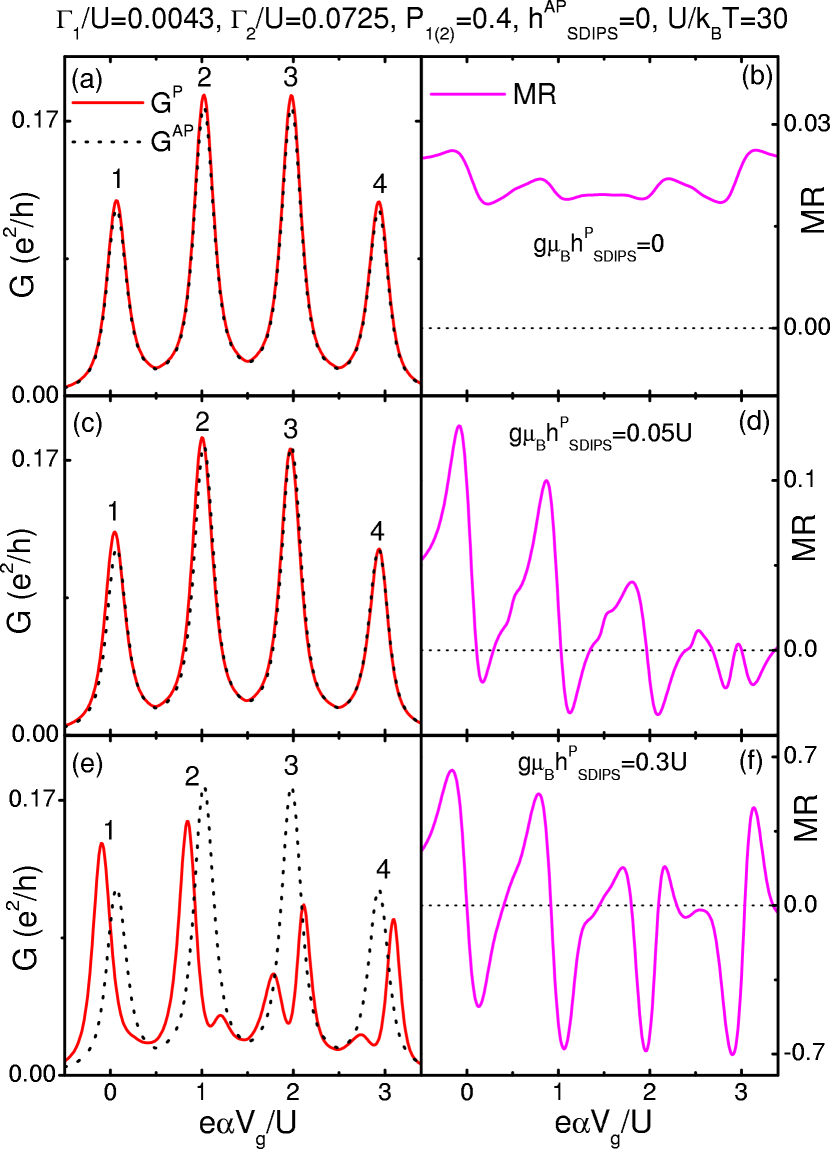
Figure 4: Panels a, c and e: Conductance $G^{P}$ in the parallel configuration (red full lines) and conductance $G^{AP}$ in the antiparallel configuration (black dotted lines), for the circuit of Fig. 1, with M a two-orbitals quantum dot. We have used identical tunnel rates to the two orbitals, i.e. $\Gamma_{L}=0.0043U$, $\Gamma_{R}=0.0725U$, and $P_{L(R)}=0.4$. We have also used $U/k_{B}T=30$ and $h_{SDIPS}^{AP}=0$. Panels b, d and f: Magnetoresistance $\mathrm{MR}$ (pink full lines) corresponding to the left conductance plots. The results are shown for $g\mu_{B}h_{SDIPS}^{P}=0$ (panels a and b), $g\mu_{B}h_{SDIPS}^{P}=0.05U$ (panels c and d) and $g\mu_{B}h_{SDIPS}^{P}=0.3U$ (panels e and f).

$$G_{s}=\left(\hbar\omega-\xi_{s}-\Sigma_{s}^{0}\right)^{-1}\left\{\hbar+U\left(D_{s}^{s_{1}}+D_{s}^{s_{2}}+D_{s}^{s_{3}}\right)\right\}$$ (12)

$$D_{s}^{s_{1}} =\left(\hbar\omega-\xi_{s}-U-\Sigma_{s}^{0}-\Sigma_{s,s_{1}}^{3,1}\right)^{-1}\left\{\hbar\left\langle n_{s_{1}}\right\rangle-\Sigma_{s,s_{1}}^{1,1}G_{s}\right.$$

$$+\left(U-\chi_{s,s_{1}}^{3,1}\right)\left(D_{s}^{s_{1},s_{2}}+D_{s}^{s_{1},s_{3}}\right)+\chi_{s,s_{1}}^{1,1}\left(D_{s}^{s_{2}}+D_{s}^{s_{3}}\right)$$

$$+\left.\left(\chi_{s,s_{1}}^{1,3}-\chi_{s,s_{1}}^{1,1}\right)D_{s}^{s_{2},s_{3}}+\left(\chi_{s,s_{1}}^{3,1}-\chi_{s,s_{1}}^{3,3}\right)D_{s}^{s_{1},s_{2},s_{3}}\right\}$$ (13)

$$D_{s}^{s_{1},s_{2}} =\left(\hbar\omega-\xi_{s}-2U-\Sigma_{s}^{0}-\Sigma_{s,s_{1}}^{3,3}-\Sigma_{s,s_{2}}^{3,3}\right)^{-1}$$

$$\left\{\hbar\left\langle n_{s_{1}}n_{s_{2}}\right\rangle-\Sigma_{s,s_{1}}^{1,3}D_{s}^{s_{2}}-\Sigma_{s,s_{2}}^{1,3}D_{s}^{s_{1}}+\chi_{s,s_{1}}^{1,3}D_{d\sigma}^{s_{2},s_{3}}\right.$$

$$\left.+\chi_{s,s_{2}}^{1,3}D_{s}^{s_{1},s_{3}}+\left(U-\chi_{s,s_{1}}^{3,3}-\chi_{s,s_{2}}^{3,3}\right)D_{s}^{s_{1},s_{2},s_{3}}\right\}$$ (14)

$$D_{s}^{s_{1},s_{2},s_{3}} =\left(\hbar\omega-\xi_{s}-3U-\Sigma_{s}^{0}-\Sigma_{s,s_{1}}^{3,5}-\Sigma_{s,s_{2}}^{3,5}-\Sigma_{s,s_{3}}^{3,5}\right)^{-1}$$

$$\left\{\hbar\left\langle n_{s_{1}}n_{s_{2}}n_{s_{3}}\right\rangle\right.$$

$$\left.-\Sigma_{s,s_{1}}^{1,5}D_{s}^{s_{2},s_{3}}-\Sigma_{s,s_{2}}^{1,5}D_{s}^{s_{3},s_{1}}-\Sigma_{s,s_{3}}^{1,5}D_{s}^{s_{1},s_{2}}\right\}$$ (15)

Due to interaction $U$, the Green’s function $G_{s}=G_{s}(\omega)$ is coupled to other Green’s functions $D_{s}^{s_{1},...,s_{3}}(\omega)=\int_{-\infty}^{+\infty}\widetilde{D}_{s}^{s_{1},...,s_{3}}(\omega)e^{i\omega t}dt$ with $\widetilde{D}_{s}^{s_{1},..,s_{{}_{3}}}(t)=-i\theta(t)\langle\{n_{s_{1}}(t)..n_{s_{3}}(t)c_{s}(t),c_{s}^{\dagger}\}\rangle$ and $n_{s_{i}}(t)=c_{s_{i}}^{\dagger}(t)c_{s_{i}}(t)$ for $i\in\{1,3\}$. This means that the dynamics of electrons in state $s$ is modified by the presence of other electrons on the dot [In the one orbital case, $G_{d\sigma}$ was coupled to $D_{d\sigma}^{d\overline{\sigma}}$ only, which lead to simple expression (4)]. The term $\Sigma_{s}^{0}=-i(\Gamma_{s}^{L}+\Gamma_{s}^{R})/2$ is the tunneling self energy for a non-interacting quantum dot, already introduced in previous section. The equations of motion also involve terms $\Sigma_{d\sigma,d^{\prime}\sigma^{\prime}}^{i,n}$, which are defined by Eq.(9), and terms defined by

$$\chi_{d\sigma,d^{\prime}\sigma^{\prime}}^{i,n}=\sum\limits_{k}\left(\frac{\mu_{i}(\xi_{k\sigma^{\prime}})\left|t_{k\sigma^{\prime}}^{d^{\prime}}\right|^{2}}{\hbar\omega-\xi_{d\sigma}-\xi_{d^{\prime}\sigma^{\prime}}+\xi_{k\sigma^{\prime}}-nU+i0^{+}}\right.\\ \left.-\frac{\mu_{i}(\xi_{k\sigma^{\prime}})\left|t_{k\sigma^{\prime}}^{d^{\prime}}\right|^{2}}{\hbar\omega-\xi_{d\sigma}-\xi_{d^{\prime}\sigma^{\prime}}+\xi_{k\sigma^{\prime}}-(n+2)U+i0^{+}}\right)$$ (16)

These terms take into account the tunneling of electrons between the leads and a dot state $d^{\prime}\sigma^{\prime}$ different from $d\sigma$. The average level occupations occuring in Eqs. (12)–(15) are given by $\left\langle n_{s_{1}},..,n_{s_{n}}\right\rangle=-\int_{-\infty}^{+\infty}\frac{d\omega}{\pi}f(\hbar\omega)\operatorname{Im}[D_{n_{s_{n}}}^{s_{1},..,s_{n-1}}(\omega)]$. The Green’s functions and the level occupations can be calculated numerically from the above equations. Up to now, the E.O.M. technique for multilevel systems had been implemented only by neglecting $\Sigma_{d\sigma,d^{\prime}\sigma^{\prime}}^{i,n}$ and $\chi_{d\sigma,d^{\prime}\sigma^{\prime}}^{i,n}$ terms multi . Like in the one-orbital case, these terms are not negligible in the context of our study.

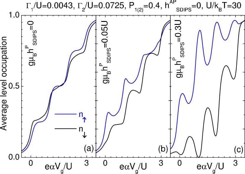
Figure 5: Average occupations $\left\langle n_{\uparrow}\right\rangle=\left\langle n_{K\uparrow}\right\rangle=\left\langle n_{K^{\prime}\uparrow}\right\rangle$ (blue lines) and $\left\langle n_{\downarrow}\right\rangle=\left\langle n_{K\downarrow}\right\rangle=\left\langle n_{K^{\prime}\downarrow}\right\rangle$ (black lines) of levels $K$ and $K^{\prime}$ by spins $\uparrow$ and $\downarrow$ as a function of $V_{g}$, for a two-orbitals quantum dot circuit with the same parameters as in Fig. 4. The results are shown for lead polarizations in the parallel configuration ($c=P$), with $h_{SDIPS}^{P}=0$ (panel a), $g\mu_{B}h_{SDIPS}^{P}=0.05U$ (panel b), and $g\mu_{B}h_{SDIPS}^{P}=0.3U$ (panel c). For $h_{SDIPS}^{P}=0$, $\left\langle n_{\uparrow}\right\rangle$ and $\left\langle n_{\downarrow}\right\rangle$ remains very close, showing four steps corresponding to the four conductances peaks visible in Fig. 4-a. In the case of a finite $h_{SDIPS}^{P}$, $\left\langle n_{\uparrow}\right\rangle$ rises more strongly than $\left\langle n_{\downarrow}\right\rangle$ for the two first conductance peaks, which shows that current transport is due in majority to up spins for these two peaks. The opposite situation occurs for the two last conductance peaks. The asymmetry between the behaviors of spins $\uparrow$ and $\downarrow$ increases with $h_{SDIPS}^{P}$ (from left to right panels).

Figure 4 shows the conductance (panels a, c and e) and $\mathrm{MR}$ curves (panels b, d and f) calculated from Eqs. (3) and (12-15), for different values of $h_{SDIPS}^{c}$. For simplicity, we have assumed that the coupling to the leads is identical for the two orbitals, i.e. $\Gamma_{K\uparrow[\downarrow]}^{l}=\Gamma_{K^{{}^{\prime}}\uparrow[\downarrow]}^{l}=\Gamma_{l}(1\pm P_{l})$ for $l\in\{L,R\}$. We have again used parameters consistent with Ref. Sahoo, i.e. $U/k_{B}T=30$, relatively low polarizations $\left|P_{L(R)}\right|=0.4$ and values of $\Gamma_{L(R)}$ leading to the proper width and height for the conductance peaks. We have checked that these parameters are compatible with the hypothesis $T>T_{K}$, with $T_{K}$ the Kondo temperature associated to the SU(4) Kondo effect expected in this system SU4th . In most cases, the curves $G^{c}(V_{g})$ show 4 resonances, the first two associated with a single occupation of $K$ and $K^{\prime}$, and the other two to double occupation (see e.g. Fig. 4-a). For $h_{SDIPS}^{P}=h_{SDIPS}^{AP}=0$ and the parameters used here, $\mathrm{MR}$ remains positive for any value of $V_{g}$ (Fig. 4-b). Like in the 1-orbital case, a finite $h_{SDIPS}^{c}$ makes easier negative $\mathrm{MR}$ effects and can even lead to a giant $\mathrm{MR}$ effect with a sign tunable with $V_{g}$ (Figs 4-d and 4-f). Importantly, the effect of $h_{SDIPS}^{c}$ depends on the occupation of the dot. For instance, in Fig. 4-e plotted for $g\mu_{B}h_{SDIPS}^{P}$ larger than the linewidth of the conductance peaks, the first two conductance peaks of $G^{P}$ (peaks 1 and 2) are strongly shifted to the left by $h_{SDIPS}^{P}$ because they are due in majority to up spins, as can be seen from the average occupation of the levels in Fig. 5-c. This allows to get a $\mathrm{MR}$ pattern approximately similar for these two peaks, i.e. a transition from positive to negative values of $\mathrm{MR}$ (Fig. 4-f). On the contrary, peak 4 corresponds to a transition from negative to positive values of $\mathrm{MR}$ because the associated conductance peak is due in majority to down spins. In Fig. 4-e, the shape of the $\mathrm{MR}(V_{g})$ pattern associated to peak 3 is more particular (positive/negative/positive) because, for the values of parameters considered here, Coulomb blockade does not entirely suppress the up spins contribution in peak 3, which is therefore spin-split MoreSym . Remarkably, this allows to obtain, at the left of Fig. 4-f, three positive $\mathrm{MR}$ maxima which differ in amplitude but have rather similar shapes. In the case of $g\mu_{B}h_{SDIPS}^{P}$ finite but smaller than the linewidth of the conductance peaks (Fig. 4-c), the amplitude of the $\mathrm{MR}$ signal is much smaller than in the previous case but its shape remains comparable.

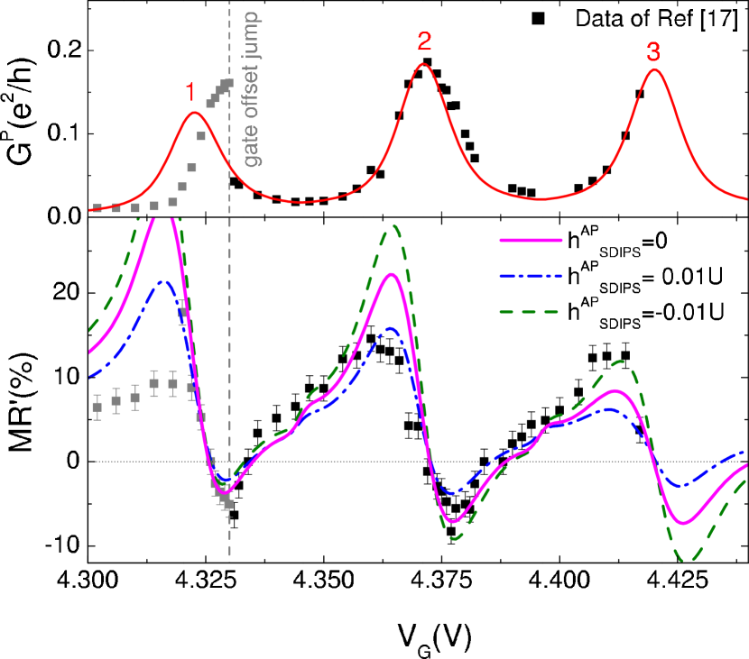
Figure 6: Comparison between the data of Ref. Sahoo, (squares) and the two-orbitals theory. We show the conductance $G^{P}$ in the parallel configuration (top panel) and the corresponding magnetoresistance $\mathrm{MR}^{\prime}=(G^{P}-G^{AP})/G^{AP}$ (bottom panel). The theory is shown for parameters consistent with the experiment i.e. $U=5~{}\mathrm{meV}$, $U/k_{B}T=30$ and $\alpha=0.0986$. We also use relatively low values of polarization $P_{L(R)}=0.4$ because usual ferromagnetic contact materials are not fully polarized Soulen . Assuming identical tunnel couplings for the two orbitals, the values of tunnels rates $\Gamma_{L}=0.0043U$ and $\Gamma_{R}=0.0725U$ are imposed by the width and height of the conductance peaks. Then, $h_{SDIPS}^{P[AP]}$ are the only free fitting parameters which remain for interpreting the $\mathrm{MR}$ curve. We have assumed $g\mu_{B}h_{SDIPS}^{P}=0.05U$ for all the theoretical curves shown in this Figure. We have plot the $MR$ curves of bottom panel for $h_{SDIPS}^{AP}=0$ (pink curve, corresponding to Fig. 4-d), $h_{SDIPS}^{AP}=-0.01U$ (green dashed curve) and $h_{SDIPS}^{AP}=0.01U$ (blue dot-dashed curve). Note that in this Figure, we show $MR^{\prime}$ instead of $MR=(G^{P}-G^{AP})/(G^{P}+G^{AP}$ $)$ in order to be consistent with Ref.  Sahoo, . A strong gate voltage offset jump occurred at $V_{g}=4.331~{}$V, therefore, we show the data at the left/right of this jump with grey/black symbols.

We now reconsider the experimental data of Ref. Sahoo, . Even the two-orbital model cannot not provide a reasonable fit to the data if we assume $h_{SDIPS}^{P}=0$ and $h_{SDIPS}^{AP}=0$. In contrast, the two-orbital model exhibits a good agreement with the experimental data for $h_{SDIPS}^{P}=0.05U$, $h_{SDIPS}^{AP}=0$, $\Gamma_{L}/U=0.0043$, $\Gamma_{R}/U=0.0725$, $\left|P_{L(R)}\right|=0.4$, and parameters $U=5~{}meV$, $U/k_{B}T=30$, and $\alpha=0.0986$ given by the experiment (see Fig. 6, red and pink full curves).

We now discuss the value of $h_{SDIPS}^{P}=0.05U$ found for the above fit. This corresponds to a magnetic field of about $2~{}\mathrm{T}$, which is too strong to be attributed to stray fields from the ferromagnetic electrodes (see e.g. Ref. stray, ). This is in favor of generalizing the SDIPS concept to SWNTs quantum dots circuits, i.e. considering that the energy levels of the dot are spin-split because the confinement potential created by the ferromagnetic electrodes is spin-dependent. For comparison, we have estimated $h_{SDIPS}^{P}$ in the non-interacting theorywire2005 , using realistic parameters i.e leads with a Fermi energy $10$ eV and a density of states polarized by $40\%$, and a nanotube with Fermi wavevector $8.5$ $10^{9}\mathrm{m}^{-1}$, Fermi velocitybockrath $v_{F}^{M}=8$ $10^{5}\mathrm{m.s}^{-1}$, length $L=500$ nm like in Ref. Sahoo, , and density of states $N_{F}^{M}=2L/\pi\hbar v_{F}^{M}$. We have modeled the interfaces between the nanotube and the leads with Dirac potential barriersnote , with a height which is spin-polarized by $40\%$ and an average value which corresponds toRelModel $\Gamma_{L(R)}=$ $T_{L(R)}/2\pi N_{F}^{L(R)}\sim 60$ $\mathrm{\mu}$eV (For comparison the fitting parameters used in Fig. 6 correspond to $\Gamma_{L}=21$ $\mathrm{\mu}$eV and $\Gamma_{R}=362$ $\mathrm{\mu}$eV). We obtain $h_{SDIPS}^{P}\sim 1.3~{}\mathrm{T}$, which is consistent with the above analysis.

In the above discussion, we have assumed $h_{SDIPS}^{AP}=0$ for simplicity. The height of the conductance peaks in the data imposes to use a strong assymetry $\Gamma_{R}/\Gamma_{L}\sim 17$ between the left and right tunnel rates. Thus, the two tunnel barriers are not symmetric, and there is no fundamental reason to assume $h_{SDIPS}^{AP}=0$. Figure 6 shows examples of $MR$ curves plotted for a finite $h_{SDIPS}^{AP}$. Using $h_{SDIPS}^{AP}=0.01U$ (green dashed curve) enhances the fit of the $MR$ at peak 2 whereas $h_{SDIPS}^{AP}=-0.01U$ (blue dot-dashed curve) enhances the fit of the $MR$ at peak 3. Interestingly, with the non-interacting model, assuming the most simple situation in which $\varphi_{l}^{P,\uparrow}-\varphi_{l}^{P,\downarrow}$ has the same sign for the two leads, one finds $\left|h_{SDIPS}^{AP}\right|<\left|h_{SDIPS}^{P}\right|$, which is in agreement with the values used here. The fact that the best fit for the $MR$ patterns at peaks 2 and 3 correspond to different values of $h_{SDIPS}^{AP}$ might be due to a gate dependence of the SDIPS. This is indeed possible since the potential profile of the interfaces between the wire and the leads can vary with $V_{g}$.

We now comment briefly on the data taken for $V_{g}<4.331~{}$V. It is not sure that the data shown before and after $V_{g}=4.331~{}$V correspond to the filling of consecutive levels because of the gate voltage jump which occured at this value of $V_{g}$. Nevertheless, the shape of the MR curve corresponding to $V_{g}<4.331~{}$V is rather consistent with the theory shown in Fig. 4. This suggests that these data really correspond to peak 1. At this stage, it is important to point out that other orbital levels not taken into account in our calculation should slightly modify the conductance peaks 1 and 4. The discrepancy between the theory and the data for $V_{g}<4.331~{}$V could be explained by the effect of the other orbitals. For the data at $V_{g}>4.331~{}$V, our fit is more quantitative since we have used peaks 2 and 3 of the theory.

In principle, the modelisation of the orbital levels in SWNTs can be refined by taking into account an exchange energy $J$ which favors spin alignment, an excess Coulomb energy $\delta U$ related to the double occupation of the same orbital, and a subband mismatch $\delta=\xi_{K^{\prime}\sigma}-\xi_{K\sigma}\neq 0$ (see Ref. Oreg, ). In practice, $\delta U$ is rather small but $J$ and $\delta$ can be of the same order as $U$. Two different regimes of parameters can occur in practice. If $\delta>J+\delta U+\left|g\mu_{B}h_{SDIPS}^{c}\right|$, two electrons with opposite spins will fill consecutively the same energy level while $V_{g}$ increases (see Refs. Sapmaz, ; Moriyama, ), and the behavior of the device should thus be analogue to the non-degenerate multi-orbital case evoked at the end of section III. Nevertheless, if $\delta<J+\delta U+\left|g\mu_{B}h_{SDIPS}^{c}\right|$, peaks 1 and 2 [3 and 4] will correspond in majority to the same spin direction, as observed experimentally by Liang, ; Jarillo, . In this case, the effect of $h_{SDIPS}^{c}$ should be qualitatively the same as described in the present section. We expect that the weights of K and K’ in peaks 1 and 2 differ due to $\delta\neq 0$, but this should not change the way in which $h_{SDIPS}^{c}$ shifts the conductance peaks from $P$ to $AP$.

In future experiments, it would be interesting to obtain continuous data on a larger $V_{g}$-range, in order to check that the shape of the $MR(V_{g})$ pattern depends on the occupation of the dot. This would also allow to study the gate voltage dependence of $h_{SDIPS}^{c}$. It would also be interesting to engineer contacts with ferromagnetic insulators or highly polarized ferromagnets in order to observe the SDIPS-induced giant $MR$ effect. Note that although we have considered here the limit $k_{B}T\lesssim\Gamma_{d\sigma}^{L}+\Gamma_{d\sigma}^{R}$, a strong enough SDIPS should also affect the behavior of the quantum dot in the sequential tunneling limit $k_{B}T\gg\Gamma_{d\sigma}^{L}+\Gamma_{d\sigma}^{R}$, through an analogous mechanism.

V Conclusion

Using an Anderson model, we have studied the behavior of a quantum dot connected to ferromagnetic leads through spin-active interfaces. The spin activity of the interfaces makes easier negative magnetoresistance ($\mathrm{MR}$) effects and can even lead to a giant $\mathrm{MR}$ with a sign oscillating with the gate voltage of the dot. Due to Coulomb blockade, the $\mathrm{MR}$ versus gate voltage pattern cannot be identical for all conductance peaks. It is nevertheless possible to account for the $\mathrm{MR}$ data measured by Ref. Sahoo, in single-wall carbon nanotubes by taking into account the $K-K^{\prime}$ orbital degeneracy commonly observed in those systems.

References

- (1) G. Prinz, Science 282, 1660 (1998).
- (2) S. Datta and B. Das, Appl. Phys. Lett. 56, 665 (1990).
- (3) Th. Schäpers, J. Nitta, H. B. Heersche, and H. Takayanagi, Phys. Rev. B 64, 125314 (2000); S. Krompiewski, R. Gutiérrez, and G. Cuniberti, Phys. Rev. B 69, 155423 (2004).
- (4) A. Brataas, Y.V. Nazarov, and G. E. W. Bauer, Phys. Rev. Lett. 84, 2481 (2000); D.H. Hernando, Y.V. Nazarov, A. Brataas, and G.E.W. Bauer, Phys. Rev. B 62, 5700 (2000); A. Brataas, Y.V. Nazarov and G.E.W. Bauer, Eur. Phys. J. B 22, 99 (2001).
- (5) L. Balents and R. Egger, Phys. Rev. Lett. 85, 3464 (2000); Phys. Rev. B 64, 035310 (2001).
- (6) W. Wetzels, G. E. W. Bauer, and M. Grifoni, Phys. Rev. B 72, 020407(R) (2005).
- (7) C. Ciuti, J.P. McGuire and L.J. Sham, Phys. Rev. Lett. 89, 156601 (2002), J.P. McGuire, C. Ciuti and L.J. Sham, cond-mat/0302088.
- (8) A. Brataas, G. E.W. Bauer, and P. J. Kelly, Phys. Rep. 427, 157 (2006).
- (9) A. Millis, D. Rainer, and J. A. Sauls, Phys. Rev. B 38, 4504 (1988); M. Fogelström, ibid. 62, 11812 (2000); J.C. Cuevas and M. Fogelström, ibid. 64, 104502 (2001); N.M. Chtchelkatchev, W. Belzig, Y.V. Nazarov, and C. Bruder, JETP Lett. 74, 323 (2001); D. Huertas-Hernando,Y.V. Nazarov, and W. Belzig, Phys. Rev. Lett. 88, 047003 (2002); J. Kopu, M. Eschrig, J. C. Cuevas, and M. Fogelström, Phys. Rev. B 69, 094501 (2004); E. Zhao, T. Löfwander, and J. A. Sauls, ibid. 70, 134510 (2004).
- (10) T. Tokuyasu, J. A. Sauls and D. Rainer, Phys. Rev. B 38, 8823 (1988).
- (11) A. Cottet and W. Belzig, Phys. Rev. B 72, 180503(R) (2005).
- (12) P. M. Tedrow, J. E. Tkaczyk and A. Kumar, Phys. Rev. Lett. 56, 1746 (1986).
- (13) T. Kontos, M. Aprili, J. Lesueur, and X. Grison, Phys. Rev. Lett. 86, 304 (2001); T. Kontos, M. Aprili, J. Lesueur, F. Genêt, B. Stephanidis, and R. Boursier, ibid. 89, 137007 (2002).
- (14) A. Cottet, T. Kontos, W. Belzig, C. Schönenberger and C. Bruder, Europhys. Lett. 74, 320 (2006).
- (15) Very recently, Man et al. Morpurgo have reported a spin-dependent transport experiment through a SWNT connected to collinearly-polarized ferromagnetic leads in the resonant tunneling regime. The data of this Ref. are interpreted following the lines in Ref. wire2005, . In this particular experiment, the SDIPS has been found to be vanishing. This is probably due to the fact that, considering the strong values of in this experiment, the effects of SDIPS on the curves are too weak to be resolved in the actual experiment.
- (16) H.T. Man, I.J.W. Wever and A.F. Morpurgo, cond-mat/0512505.
- (17) S. Sahoo, T. Kontos, J. Furer, C. Hoffmann, M. Graber, A. Cottet and C. Schönenberger, Nature Phys. 1, 99 (2005).
- (18) In Ref. Sahoo, , the experimental data are compared with a non-interacting theory which corresponds to the low transmission limit of Ref. wire2005, .
- (19) S. J. Tans, M. H. Devoret, J. A. Groeneveld and C. Dekker, Nature 394, 761 (1998).
- (20) S. Sapmaz, P. Jarillo-Herrero, J. Kong, C. Dekker, L. P. Kouwenhoven, and H. S. J. van der Zant, Phys. Rev. B 71, 153402 (2005).
- (21) J. Barnas and A. Fert, Phys. Rev. Lett. 80, 1058 (1998); A. Braatas, Yu. V. Nazarov, J. Inoue and G. E. W. Bauer, Phys. Rev. B 59, 93 (1999); H. Imamura, S. Takahashi and S. Maekawa, Phys. Rev. B 59, 6017 (1999); B. R. Bulka, Phys. Rev. B 62, 1186 (2000); A. Cottet, W. Belzig and C. Bruder, Phys. Rev. Lett. 92, 206801 (2004), Phys. Rev. B 70, 115315 (2004); H.-F. Mu, G. Su, and Q.-R. Zheng, Phys. Rev. B 73, 054414 (2006).
- (22) M. Braun, J. Konig and J. Martinek, Phys. Rev. B 70, 195345 (2004).
- (23) I. Weymann, J. König, J. Martinek, J. Barnas and G. Schon, Phys. Rev. B 72 115334 (2005).
- (24) N. Sergueev, Q.-F. Sun, H. Guo, B. G. Wang, and J. Wang, Phys. Rev. B 65, 165303 (2002); J. Martinek, M. Sindel, L. Borda, J. Barnas, J. König, G. Schön, and J. von Delft, Phys. Rev. Lett. 91, 247202 (2003); M.-S. Choi , D. Sanchez and R. Lopez, Phys. Rev. Lett. 92, 056601 (2004); Y. Utsumi, J. Martinek, G. Schön, H. Imamura and S. Maekawa, Phys. Rev. B 71, 245116 (2005); J. Martinek, M. Sindel, L. Borda, J. Barnas, R. Bulla, J. König, G. Schön, S. Maekawa and J. von Delft, Phys. Rev. B 72, 121302(R) (2005); R. Swirkowicz , M. Wilczynski, M. Wawrzyniak and J. Barnas, Phys. Rev. B 73, 193312 (2006).
- (25) J. Martinek, Y. Utsumi, H. Imamura, J. Barnas, S. Maekawa, J. Konig and G. Schon, Phys. Rev. Lett. 91, 127203 (2003).
- (26) C. S. Peça, L. Balents and K. J. Wiese, Phys. Rev. B 68, 205423 (2003).
- (27) H.-F. Mu, G. Su, Q.-R. Zheng, and B. Jin, Phys. Rev. B 71, 064412 (2005).
- (28) W. Liang, M. Bockrath, and H. Park, Phys. Rev. Lett. 88, 126801 (2002);
- (29) P. Jarillo-Herrero, J. Kong, H. S. J. van der Zant, C. Dekker, L. P. Kouwenhoven, and S. De Franceschi, Phys. Rev. Lett. 94, 156802 (2005).
- (30) S. Moriyama, T. Fuse, M. Suzuki, Y. Aoyagi, and K. Ishibashi, Phys. Rev. Lett. 94, 186806 (2005);
- (31) B. Babic and C. Schönenberger, Phys. Rev. B 70, 195408 (2004);
- (32) B. Babic, T. Kontos, and C. Schönenberger, Phys. Rev. B 70, 235419 (2004)
- (33) Ya. M. Blanter and M. Büttiker, Phys. Rep. 336, 1 (2000).
- (34) L. F. Schelp, A. Fert, F. Fettar, P. Holody, S. F. Lee, J. L. Maurice, F. Petroff, and A. Vaures, Phys. Rev. B 56, R5747 (1997); K. Yakushiji, S. Mitani, K.Takanashi, S. Takahashi, S. Maekawa, H. Imamura, and H. Fujimori Appl. Phys. Lett.78, 515 (2001); L. Zhang, C. Wang, Y. Wei, X. Liu, and D. Davidovic, Phys. Rev.B 72, 155445 (2005).
- (35) M.M. Deshmukh and D. C. Ralph, Phys. Rev. Lett. 89, 266803 (2002).
- (36) K. Tsukagoshi, B. W. Alphenaar, and H. Ago, Nature 401, 572574 (1999); B. Zhao, I.Mönch, H. Vinzelberg, T. Mühl and C. M. Schneider, Appl. Phys. Lett. 80, 31443146 (2002).
- (37) A. Pasupathy et al., Science 306, 86 (2004).
- (38) Note that Ref. Wetzels, has also introduced an effective exchange field to take into account the SDIPS in an interacting single electron transistor connected to ferromagnetic leads. These authors have studied precession effects produced by the SDIPS in non-collinear configurations. They did not consider spin-dependent resonance effects because this is not relevant in the diffusive limit considered in this Ref.
- (39) Y. Meir and N.S. Wingreen, Phys. Rev. Lett. 68, 2512 (1992).
- (40) Y. Meir, N.S. Wingreen and P.A. Lee, Phys. Rev. Lett., 66, 3048 (1991).
- (41) Note that in the limit considered in this article, the spin accumulation concept of Ref. FNF, simply corresponds to having a finite average spin on the quantum dot. This feature is intrinsically taken into account in our treatment.
- (42) For , the conductance given by Eqs. (3) and (4) can be perfectly mapped onto the interactionless conductance found in Ref.wire2005, for and a level close to resonance, using and .
- (43) R. J. Soulen Jr., J. M. Byers, M. S. Osofsky, B. Nadgorny, T. Ambrose, S. F. Cheng, P. R. Broussard, C. T. Tanaka, J. Nowak, J. S. Moodera, A. Barry, and J. M. D. Coey, Science 282, 85, (1998).
- (44) From Ref.Martinek , for , the Kondo temperature of the circuit is very close to the corresponding to in both the and configurations.
- (45) I.L. Aleiner, P.W. Brouwer and L.I. Glazman, Phys. Rep. 358, 309 (2002).
- (46) T. Kontos has communicated us two extra points at V.
- (47) We point out that this splitting effect is unrelated to . This is particularly clear in the limit of no tunneling , in which the renormalization of the levels by the terms vanishes whereas persists.
- (48) The function is resonant at and . Interestingly, for , , and , a simplified expression of the resonance spin-splitting caused by the terms can be obtained by evaluating at and at . This leads to where the prime represents Cauchy’s principal value. Interestingly, this expression perfectly matches with Eq. (3.9) of Ref. Braun, . This Ref. studies the precession effect produced by in a quantum dot with ferromagnetic leads polarized in non-collinear directions, in the limit . The system is described with Eqs. which neglect in the collinear case.
- (49) P. Jarillo-Herrero, J. Kong, H. S. J. van der Zant, C. Dekker, L. P. Kouwenhoven and S. De Franceschi , Nature 434, 484 (2005).
- (50) M.-S. Choi, R. López and R. Aguado, PRL 95, 67204 (2005).
- (51) We expect that the effect of the SDIPS is only quantitatively modified when these processes occur.
- (52) P. Pals and A. MacKinnon, J. Phys. Condens. Matter 8, 5401 (1996), J.J. Palacios, L. Liu and D. Yoshioka, Phys. Rev. B 55, 15735 (1997).
- (53) Note that it is possible to decrease the up spins contribution in peak 3 and to have a pattern similar for peaks 3 and 4 by using values of much smaller than in Fig.4 (e.g. ).
- (54) B. W. Alphenaar, K. Tsukagoshi and M. Wagner, J. Appl. Phys. 89, 6863 (2001).
- (55) W. Liang, M. Bockrath, D. Bozovic, J.H. Hafner, M. Tinkham and H. Park, Nature, 411, 665 (2001).
- (56) See Fig. 1 of Ref. wire2005,
- (57) Y. Oreg, K. Byczuk and B.I. Halperin, Phys. Rev. Lett. 85, 365 (2000).