Efficiency analysis of reaction rate calculation methods using analytical models I: The 2D sharp barrier

Abstract

We analyze the efficiency of different methods for the calculation of reaction rates in the case of a simple 2D analytical benchmark system. Two classes of methods are considered: the first are based on the free energy calculation along a reaction coordinate and the calculation of the transmission coefficient, the second on the sampling of dynamical pathways. We give scaling rules for how this efficiency depends on barrier height and width, and we hand out simple optimization rules for the method-specific parameters. We show that the path sampling methods, using the transition interface sampling technique, become exceedingly more efficient than the others when the reaction coordinate is not the optimal one.

I introduction

As Molecular dynamics (MD) is limited to microscopic systems and time scales, most chemical or biological reactions can not be simulated using straightforward MD. One can literally wait ages before detecting a single event in a typical computer simulation. In the early 1930s, Wigner and Eyring made the first attempts to overcome this problem by introducing the concept of the Transition state (TS) and the so-called TS Theory (TST) approximation E35 ; W38 . Later on, Keck Keck62 demonstrated how to calculate the dynamical correction, the transmission coefficient. This work has later been extended by Bennett Bennet77 , Chandler DC78 and others Yamamoto60 ; H38 , resulting in a two-step approach. First the free energy as function of a reaction coordinate (RC) is determined. This can be done by e.g. Umbrella Sampling (US) TV74 or Thermodynamic Integration (TI) CCH89 . Then, the maximum of this free energy profile defines the approximate TS dividing surface and the transmission coefficient can be calculated by releasing dynamical trajectories from the top. This approach is, in principle, exact and independent of the choice of RC. However, the method becomes inefficient when the transmission coefficient is small. A proper choice of the RC can maximize the transmission coefficient and is hence crucial for the efficiency of the method.

There exist different formalisms for the transmission coefficient formula which differ in the way trajectories are counted. We discuss the standard Bennett-Chandler (BC) DC78 , the history dependent BC (BC2) DC78 , and the effective positive flux (EPF) Anderson95 ; ErpBol2004 formalism. We show that the latter should always be preferred due to a lower average pathlength and a faster convergence. However, whenever a lot of correlated recrossings occur, the transmission coefficient will be very low and all these methods become inefficient. In high dimensional complex systems it can be a very difficult task to find a proper RC. Moreover, whenever the dynamics is diffusive, even an optimal RC can result in a very low transmission and hence a poor efficiency.

A new approach came with Transition Path Sampling (TPS) TPS98 that is not based on the free energy barrier as starting point. TPS is rather an importance sampling of dynamical trajectories. Hence, it is a Monte Carlo (MC) sampling in path space rather than phase space. The TPS method has been advocated as a method that does not need a RC and is akin to ’throwing ropes in the dark’ Bolhuis02 . This might be true if one wants to sample a set of reactive trajectories, but it is not for the calculation of reaction rates. In fact, the original approach to calculate reaction rates within the framework of TPS required the definition of an order parameter and the calculation of the reversible work when the endpoint of the path is dragged along this parameter. For the sampling of reactive pathways, the order parameter needs only to distinguish between the two stable states. However, in the algorithmic procedure to calculate reaction rates with TPS, the order parameter becomes very similar to a RC. Still, it has been speculated that this approach is less sensitive to the problems related to an improper RC (or order parameter). Indeed, in this article we prove for the first time that this is true using the approach of Transition Interface Sampling (TIS) ErpMoBol2003 . TIS increases the efficiency of the original TPS rate calculation considerably by allowing the pathlength to vary and by counting only positive effective crossings. The overall reaction rate in TIS is obtained from an importance sampling technique that uses a discrete set of interfaces between the stable states. Hence, TIS could be considered a dynamical analogue of US in path space. For diffusive systems the partial path TIS (PPTIS) was invented that uses the assumption of memory loss MoBolErp2004 . In this article we discuss the case of sharp barriers. Here recrossings occur mainly due to the wrong choice of RC. In a follow-up article we will treat the diffusive case.

Up to now, it is not clear how these methods compare in efficiency and the need for benchmark systems has been put forward several times. It is not always easy to perform comparative calculations since it is not simple to know if each method is equally optimized for a specific system. Therefore, in this paper we analyze a system for which the efficiency of the methods can be calculated analytically with only a few approximations. This does not only give a transparent comparison of the efficiency of the different methods, but also allows to obtain scaling laws for how this efficiency changes as function of the barrier height and width. Moreover, we give some rules for how the methods can be optimized, for instance, by choosing the proper width of the US windows and the position of interfaces in TIS. These rules are important for the simulation community, as they can be used as a rule of thumb in daily practice, when any method needs to be optimized.

The principal component to measure the efficiency of the methods will be the CPU efficiency time $\tau_{\rm eff}$ which is the lowest computational cost needed to obtain an overall statistical error equal to one. We give a detailed analysis of how $\tau_{\rm eff}$ can be calculated for some very general cases in the appendix sections A and  B. It also gives the important result of how one should divide a total fixed simulation time over a set of different simulations to obtain the best overall efficiency. In Sec. II, we outline the first class of methods, the reactive flux (RF) methods, and present their principal formulas. In Sec. III, we do the same for the second class of methods, the path sampling methods. Sec. IV introduces the 2D benchmark system where the angle $\theta$ indicates how far the chosen RC is deviated from the optimal one. Sec. V is the main section of our paper in which we apply the different methods of Sec. II and III to the analytical benchmark system of Sec. IV. Finally, we discuss the important point of hysteresis for the two types of methods and show that this is less likely to occur for the path sampling methods. We summarize the results in Sec. VII. Moreover, to support the readability of this paper we have added a list of symbols and abbreviations in App. E and F.

II First class of methods: Reactive Flux methods

II.1 General formalism for RF methods

In all combined free energy and transmission coefficient based methods, the rate equation follows from $k=\tilde{k}(t^{\prime})$ where the reaction rate $k$ is expressed as a quasi-plateau value at a time $t^{\prime}$ of a time dependent reaction rate function $\tilde{k}(t)$. This function is given by the corrected flux through an hypersurface $\{x|\lambda(x)=\lambda^{*}\}$, that is is a collection of phase points $x$, defined by the reaction coordinate $\lambda(x)$ and transition state (TS) value $\lambda^{*}$. The TS value $\lambda^{*}$ is standardly taken as the maximum in the free energy profile along $\lambda$. Both TST, BC, BC2 and EPF can be expressed as

$$\tilde{k}(t) =\frac{\langle\dot{\lambda}(x_{0})\delta(\lambda(x_{0})-\lambda^{*})\chi[X,t]\rangle}{\langle\theta(\lambda^{*}-\lambda(x_{0}))\rangle},$$ (1)

where $\delta(\cdot)$ is the Dirac delta function, $\theta(\cdot)$ the Heaviside step function, $x_{t}$ is the phase point at a time $t$, and $X$ is a trajectory that includes $x_{0}$. Ensemble averages $\langle\ldots\rangle$ in phase and path space are defined in App. A.1. Eq. (1) measures the flux contributed by pathways leaving the surface $\lambda^{*}$ at $t=0$ under the influence of a correction functional $\chi[X,t]$. The functional $\chi$ has different forms for TST, BC, BC2, and EPF. The rate equation (1) can be rewritten as a product of two factors: the probability to be on top of the barrier times the transmission function $\tilde{\mathcal{R}}(t)$:

$$\tilde{k}(t) =P_{A}(\lambda^{*})\tilde{\mathcal{R}}(t)$$ (2)

with

$$P_{A}(\lambda^{*}) \equiv\frac{\langle\delta(\lambda(x_{0})-\lambda^{*})\rangle}{\langle\theta(\lambda^{*}-\lambda(x_{0}))\rangle}.$$ (3)

and

$$\tilde{\mathcal{R}}(t) \equiv\langle\dot{\lambda}(x_{0})\chi[X,t]\rangle_{\delta(\lambda(x_{0})-\lambda^{*})}.$$ (4)

Here, $\langle\ldots\rangle_{\delta(\lambda(x_{0})-\lambda^{*})}$ implies that the ensemble $\{x_{0}\}$ is constrained at the surface $\{x_{0}|\lambda(x_{0})=\lambda^{*}\}$. Substitution of Eqs. (4,3) in Eq. (2) using Eq. (70) gives back Eq. (1).

Eqs. (2-3) show the two-step procedure. The probability $P_{A}(\lambda^{*})$ and the time dependent transmission function $\tilde{\mathcal{R}}(t)$ are calculated in two separate simulations. As for the rate $k$, the unnormalized transmission coefficient ${\mathcal{R}}$ follows from a plateau in this time dependent function: ${\mathcal{R}}=\tilde{\mathcal{R}}(t^{\prime})$. This factor corrects for the correlated recrossings. In II.2, we discuss the methods to compute $P_{A}(\lambda^{*})$ or, equivalently, the free energy barrier $\Delta F=-k_{B}T\ln P_{A}(\lambda^{*})$. Then, in II.3 we discuss the methods to determine the transmission coefficient ${\mathcal{R}}$.

II.2 Free energy methods

II.2.1 US using rectangular windows

Define the following $2M+2$ box functions:

$$w_{i}(x) =\theta[\lambda(x)-\lambda_{R}-i\Gamma]\theta[\lambda_{R}+i\Gamma+\gamma-\lambda(x)],$$

$$w_{M}(x) =\theta[\lambda(x)+d\lambda-\lambda^{*}]\theta[\lambda^{*}-\lambda(x)],$$

$$W_{0}(x) =\theta[\lambda^{*}-\lambda(x)],$$ (5)

$$W_{j}(x) =\theta[\lambda(x)-\lambda_{R}-(j-1)\Gamma]\theta[\lambda_{R}+j\Gamma+\gamma-\lambda(x)],$$

with $0\leq i<M$ and $0<j\leq M$. Here $\lambda^{*}$ is the TS, $\lambda_{R}$ is a value in the reactant well and $d\lambda$ is a small length scale. $\gamma$ and $\Gamma$ represent the dimensions of the US windows; $\Gamma+\gamma$ is the width of the window and $\gamma$ is the overlap such that $M\Gamma+d\lambda=\lambda^{*}-\lambda_{R}$ (See Fig. 1).

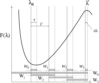
Figure 1: Illustration of US using rectangular windows for the case $M=3$. $\lambda_{R}$ is a surface in the reactant well, $\lambda^{*}$ is the TS. The binary functions $w_{i}$ and $W_{i}$ are depicted below the free energy plot where the gray areas indicate where $w_{i},W_{i}$ equal unity.

Neglecting higher orders terms in $d\lambda$, we can write

$$P_{A}(\lambda^{*}) =\frac{1}{{\mathrm{d}}\lambda}\frac{\langle w_{M}\rangle}{\langle\theta(\lambda^{*}-\lambda)\rangle}=\frac{1}{{\mathrm{d}}\lambda}\langle w_{M}\rangle_{W_{0}}.$$ (6)

To calculate Eq. (6), we can simply run an MD simulation and count the number of times that the transition state region interval is visited. The weight function $W_{0}$ in the ensemble acts like an infinite wall at $\lambda=\lambda^{*}$ and prevents the unnecessary exploration of the product region. However, as $\langle w_{M}\rangle_{W_{0}}$ is vanishingly small for high barriers, this straight-forward method will usually fail.

Using Eq. (70) and the relations $w_{s}W_{s}=w_{s}$, $w_{s-1}W_{s}=w_{s-1}$ for all $s$ we can rewrite Eq. (6) as

$$P_{A}(\lambda^{*}) =\frac{1}{{\mathrm{d}}\lambda}\langle w_{0}\rangle_{W_{0}}\prod_{s=1}^{M}\frac{\langle w_{s}\rangle_{W_{s}}}{\langle w_{(s-1)}\rangle_{W_{s}}}.$$ (7)

The final property is now calculated from a series of simulations in which each pair $\langle w_{s}\rangle_{W_{s}},\langle w_{s-1}\rangle_{W_{s}}\gg\langle w_{M}\rangle_{W_{0}}$ so that they can be determined accurately. The implementation of US using rectangular windows via MC is straightforward. The standard MC sampling is performed starting from a point inside the window. As soon as the MC procedure generates a point outside this window, this point is automatically rejected and the old point is kept. If the procedure is performed by means of MD, the window boundaries simply act as infinitely hard walls. However, due to practical problems related to a discontinuous force profile, MD simulations are usually performed with parabolic windows instead of rectangular ones.

II.2.2 US using a single biasing potential

Instead of performing several simulations using rectangular windows, one can also use a single biasing function $\Omega(x)$:

$$P_{A}(\lambda^{*}) =\frac{1}{{\mathrm{d}}\lambda}\frac{\langle w_{M}\Omega^{-1}\rangle_{\Omega W_{0}}}{\langle\Omega^{-1}\rangle_{\Omega W_{0}}}.$$ (8)

Again, the equivalence between Eq. (6) and Eq. (8) is easy to prove via Eq. (70). The advantage of Eq. (8) is that the error does not propagate as in the case of several windows. On the other hand, one needs to have already a good idea about the shape of the barrier to construct a good bias $\Omega$. The series of rectangular windows is a more robust way to explore the barrier region when no knowledge is available. The algorithmic procedure to sample points in the biased ensemble $\langle\ldots\rangle_{\Omega W_{0}}$ is explained in Sec. A.1.

II.2.3 Other free energy methods

Many other methods exist for the calculation of free energy surfaces. TI is of equally importance and is based on the constrained sampling at surfaces from which the free energy’s derivative can be obtained at a given value of $\lambda$. Integration of these derivatives results in the requested free energy profile. In addition, many variations of US have been devised, such as Wang-Landau sampling WangLandau , meta dynamics LP02 , and flooding flood , where the optimal biasing potential is created on the fly.

II.3 Transmission coefficient calculation

II.3.1 TST approximation

In TST, all pathways leading towards the product site $B$ are assumed to stay in $B$ for a very long time. The TST approximation uses Eq. (4) with

$$\chi^{\rm TST}[X,t]=\theta(\dot{\lambda}(x_{0})).$$ (9)

If the barrier is sharp and a proper RC is taken, TST is a very good approximation or can even be exact. The calculation of ${\mathcal{R}}$, in TST, requires a simple numerical or analytical calculation. For instance, suppose that $\lambda$ is a simple Cartesian coordinate with mass $m$, then $\dot{\lambda}(x_{0})=v$ and

$${\mathcal{R}}=\frac{\int_{0}^{\infty}{\mathrm{d}}v\,ve^{-\beta\frac{1}{2}mv^{2}}}{\int_{-\infty}^{\infty}{\mathrm{d}}v\,e^{-\beta\frac{1}{2}mv^{2}}}=\frac{1/\beta m}{\sqrt{2\pi/\beta m}}=\frac{1}{\sqrt{2\pi\beta m}}.$$ (10)

Therefore, the free energy profile is sufficient to obtain $k$ whenever TST is valid.

II.3.2 BC formalism

The BC equation is obtained using

$$\chi^{\rm BC}[X,t]=\theta[\lambda(x_{t})-\lambda^{*}]$$ (11)

in Eq. (4). The evaluation of $\tilde{\mathcal{R}}(t)$ in Eq. (4) consists of releasing many trajectories that start from the top of the barrier. These trajectories only make a contribution different from zero if they end up at the product side of the barrier. It is important to note that a trajectory with $\dot{\lambda}(x_{0})<0$ that leaves the surface heading to the reactant state $A$ but finally ends up at the product state $B$ at a time $t$, gives a negative contribution. The final value, which has to be positive per definition, results from a cancellation of positive and negative terms.

II.3.3 BC2 formalism

The BC2 equation uses

$$\chi^{\rm BC2}[X,t] =\theta[\lambda(x_{t})-\lambda^{*}]\theta[\lambda^{*}-\lambda(x_{-t})].$$ (12)

Here, besides ending in the product state, the trajectories integrated backward in time also have to end in the reactant state to give a nonzero contribution to Eq. (4). However, here as well, the contribution of some trajectories are negative. This happens when the systems starts with a negative $\dot{\lambda}(x_{0})$, but the forward and backward trajectories end up in the product $B$ and reactant state $A$, respectively. These so-called S-curves (trajectories that cross the TS surface more than 2 times within a short time) are less likely to occur for sharp barriers.

II.3.4 EPF formalism

The EPF equation arises when we take $\chi[X,t]=\chi^{\rm EPF}[X,t]$ in Eq. (4) with

$$\chi^{\rm EPF}[X,t] =\begin{cases}0,&\textrm{if }\dot{\lambda}(x_{0})<0,\\ &\textrm{or if }\lambda_{t^{\prime}}>\lambda^{*}\textrm{ for any }t^{\prime}\in[-t:0],\\ &\textrm{or if }\lambda(x_{t})<\lambda^{*},\\ 1,&\textrm{otherwise.}\end{cases}$$ (13)

Despite the apparent mathematical more complicated form of Eq. (13) compared to Eqs. (11) and (12), the relation is quite is natural. The approach counts only the first crossings and only when they are in the positive direction (See Fig. 2).

Figure 2: Explanation of the transmission coefficient method (11-13). The dot on the surface $\lambda^{*}$ indicates the point of release at $t=0$. The arrow indicates the direction of $\dot{\lambda}(x_{0})$. Trajectories are integrated forward up to $t=t^{\prime}$ and backward in time up to $t=-t^{\prime}$. From top to bottom, $\dot{\lambda}(x_{0})\chi$ using BC Eq. (11) results in $(v,0,v,v,v,0,-v,-v)$, the BC2 Eq. (12) gives $(v,0,0,v,v,0,0,-v)$, and the EPF expression Eq. (13) gives $(v,0,0,0,v,0,0,0$) with $v=|\dot{\lambda}(x_{0})|$ the absolute velocity at the initial point.

In the effective flux formalism (13), all contributions are either zero or positive. In Ref. [ErpBol2004, ], we presented a similar transmission coefficient formula. However, in this approach the pathway was stopped whenever the stable state regions $A$ and $B$ were reached. For a formal mathematical proof of the equivalence between BC- and EPF-type equations see Ref. [EricvE, ].

II.3.5 Other transmission coefficient methods

Some other relations for the transmission different from Eq. (11-13) have been proposed. For instance, Hummer Hummer04 proposed a relation that uses all the crossing velocities, in case of correlated recrossings, instead of just $\dot{\lambda}(x_{0})$. Ruiz-Montero et al. Ruiz devised a transition zone method for diffusive barrier crossings. This will be treated in more detail in the follow up article that will discuss the diffusive barrier case.

III Second class of methods : path sampling methods

III.1 General formalism of TIS methods

Suppose $\lambda_{A}$ and $\lambda_{B}>\lambda_{A}$ are such that any $x$ with $\lambda(x)<\lambda_{A}$ is at the reactant side $A$ and any $x$ with $\lambda(x)>\lambda_{B}$ is at the product side $B$ of the unknown optimal TS dividing surface. It is important to note that $\lambda(x)$ does not have to be a proper RC to fulfill this criterion, but only has to distinguish between the two stable states. The TIS expression is now given by

$$k_{AB} =\frac{\langle\phi_{A}\rangle}{\langle h_{\mathcal{A}}\rangle}{\mathcal{P}}_{A}(\lambda_{B}|\lambda_{A}).$$ (14)

Here $\phi_{A}$ gives the flux through interface $\lambda_{A}$ and $h_{\mathcal{A}}$ is a history dependent function describing whether the system was more recently in $A$ or in $B$: $h_{\mathcal{A}}=1$, for a phase point $x$ and its corresponding trajectory, if the system was more recently in $A$ than in $B$ and $h_{\mathcal{A}}=0$ otherwise. In practice, the whole factor $\frac{\langle\phi_{A}\rangle}{\langle h_{\mathcal{A}}\rangle}$ is calculated by counting the number of crossings in a straight-forward MD simulation, divided by the number of cycles with $h_{\mathcal{A}}=1$, divided by the time step $\Delta t$. The calculation of this factor is very cheap as interface $\lambda_{A}$ is very close to the basin of attraction of state $A$. On the other hand, the crossing probability ${\mathcal{P}}_{A}(\lambda_{B}|\lambda_{A})$ is a very small number and can not be accurately determined by straightforward MD. This is the probability that whenever the system crosses interface $\lambda_{A}$, it will cross interface $\lambda_{B}$ before crossing interface $\lambda_{A}$ again. As interface $\lambda_{B}$ is an interface at the other side of the barrier, this probability is very small. The TIS method overcomes this by defining $M-1$ interfaces between $\lambda_{A}=\lambda_{0}$ and $\lambda_{B}=\lambda_{M}$. Then, the total crossing probability can be expressed in a formula that contains conditional short-distance crossing probabilities ErpMoBol2003

$${\mathcal{P}}_{A}(\lambda_{B}|\lambda_{A})={\mathcal{P}}_{A}(\lambda_{M}|\lambda_{0}) =\prod_{s=0}^{M-1}{\mathcal{P}}_{A}(\lambda_{s+1}|\lambda_{s}).$$ (15)

Here, ${\mathcal{P}}_{A}(\lambda_{s+1}|\lambda_{s})$ is a generalization of the previously described overall crossing probability and denotes the conditional probability that, whenever the system leaves state $A$ by crossing $\lambda_{A}$ and crosses $\lambda_{s}$ in turn, it will also cross $\lambda_{s+1}$ before returning to $A$. If the distances $\lambda_{s+1}-\lambda_{s}$ are sufficiently small, the probabilities ${\mathcal{P}}_{A}(\lambda_{s+1}|\lambda_{s})$ will be large enough so that they can be computed using a shooting algorithm TPS98_2 . The shooting algorithm takes a random time slice from the old existing path and makes a slight randomized modification of this phase point (usually only the momenta are changed). Then, this new phase point is used to propagate forward and backward in time yielding a new trajectory. In TIS, this propagation of the trajectory is stopped whenever the system enters $A$ or $B$ or, equivalently, whenever $\lambda_{0}$ or $\lambda_{M}$ are crossed. The pathway is accepted only if the backward trajectory ends in $A$ and the total trajectory has at least one crossing with $\lambda_{s}$. The fraction of these paths that cross $\lambda_{s+1}$ as well, determines ${\mathcal{P}}_{A}(\lambda_{s+1}|\lambda_{s})$. Although the form of Eq. (15) deceptively resembles a Markovian factorization, no assumption has been made. As ${\mathcal{P}}_{A}(\lambda_{s+1}|\lambda_{s})$ are not simple hopping probabilities, but incorporate the full history-dependence from $\lambda_{A}$ to $\lambda_{s}$, the relation is actually non-Markovian and exact Moronithesis .

III.2 TIS biasing on $\lambda_{\max}$

In analogy with US, instead of using a discrete set of interfaces, we could also bias the trajectory in a continuous way using a bias on $\lambda_{\max}$ ErpMoBol2003 . First we can write

$${\mathcal{P}}_{A}(\lambda_{M}|\lambda_{0})=\langle\theta(\lambda_{\max}[X]-\lambda_{B})\rangle.$$ (16)

Here $\lambda_{\max}=\max\{\lambda(x_{t})|x_{t}\in X\}$ where the path $X$ is terminated when it leaves $A$ and enters region $A$ or $B$. Then, as in Eq. (8) we can write

$${\mathcal{P}}_{A}(\lambda_{M}|\lambda_{0})=\frac{\langle\theta(\lambda_{\max}[X]-\lambda_{B})\Omega^{-1}(\lambda_{\max})\rangle_{\Omega}}{\langle\Omega^{-1}(\lambda_{\max})\rangle_{\Omega}}.$$ (17)

The algorithmic procedure would be the same as TIS without the interface crossing constraint. Instead, the acceptance-rejection criterion is adjusted as explained in Sec. A.1. A continuous bias has been applied within the original TPS scheme. In Ref. [Corcelli, ] a bias on the end point of the path was used. Alternatively, one can also bias the direction of the momenta change at the shooting point as was done in Ref. [MacFayden, ].

III.3 Other path sampling methods

The original TPS rate calculation algorithm was introduced in Refs. [TPS98, ; TPS98_2, ; TPS99, ]. It first creates ensemble of reactive trajectories of a fixed length. These trajectories should constitute a time interval that is longer than $t^{\prime}$ where $\tilde{k}(t)$ reach its plateau. Then, a second series of simulations is required that combines the MC of pathways with a US technique. Also these simulations use a fixed pathlength, but these can be shorter using a rescaling approach TPS99 . In the end, the final rate constant can be constructed from the results of these two types of simulations. Moroni showed that this algorithm is always less efficient than the TIS technique and that the computational advancement of TIS is at least a factor two Moronithesis . The TIS improvement is partly due to the flexible pathlength so that each individual path can be limited to its strictly necessary minimum. Moreover, TIS has abandoned the shifting moves and has a stronger convergence (no cancellation positive and negative terms). Depending on the system and the required accuracy, the TIS approach can easily become more than an order of magnitude faster than the original approach.

The PPTIS method reduces the average pathlength even further as compared to TIS using the assumption of memory-loss MoBolErp2004 . In this method, the trajectories do not have to start at $\lambda_{A}$. Instead, an ensemble of trajectories is generated that start and end at either $\lambda_{s+1}$ or $\lambda_{s-1}$, but must have at least one crossing with the middle interface $\lambda_{s}$. From this, four crossing probabilities can be constructed that still inhibit some history dependence. Once these are known for each $s$, the final overall crossing probability can be constructed via a recursive relation MoBolErp2004 . The Milestoning method Milestoning is very similar to PPTIS, but relies on a stronger Markovian assumption that the system remains in an equilibrium distribution at each interface. On the other hand, Milestoning uses time-dependent hopping probabilities which supplies a very general way to coarse-grain a dynamical system. The two aspects of PPTIS and Milestoning could be combined as was suggested in Ref. [MoErpBol, ].

Finally, we mention Forward Flux Sampling (FFS) FFS ; FFS2 . FFS uses the same rate equation (15) as TIS, but the sampling is different. In FFS FFS ; FFS2 , the crossing points at the next interface of the ’successful pathways’ are stored. The next simulation uses this set of points to initiate new pathways. The advantage is that FFS does not require any knowledge on the distribution $\rho(x)$. This allows to treat non-equilibrium systems as well. Moreover, FFS creates effectively more pathways than TIS with the same amount of MD steps and does not rely on a Markovian assumption as in PPTIS. However, the correlation between the different pathways is much stronger than in TIS or PPTIS. Therefore, FFS can only be applied when the process is sufficiently stochastic.

IV analytical 2D benchmark system

We consider the following 2D potential:

$$V(\lambda_{x},\lambda_{y}) =\begin{cases}\infty,&\textrm{if }|\lambda_{x}-\lambda_{x}^{*}|>R_{x},\\ V_{\rm bar}(\lambda_{\perp})&\textrm{otherwise}\end{cases}$$ (18)

with

$$\lambda_{\perp}(\lambda_{x},\lambda_{y}) =(\lambda_{x}-\lambda_{x}^{*})\cos\theta-(\lambda_{y}-\lambda_{y}^{*})\sin\theta$$ (19)

and

$$V_{\rm bar}(\lambda)=\begin{cases}0,&\textrm{if }|\lambda|>\frac{1}{2}W,\\ \big{(}1-\frac{2|\lambda|}{W}\big{)}H&\textrm{if }|\lambda|<\frac{1}{2}W.\end{cases}$$ (20)

Here, $H$ is the height of our barrier, $W$ is the barrier width and $R_{x},R_{y}$ are the dimensions of the reactant region (See Fig. 3).

Figure 3: The two-dimensional potential given by Eq. (18). $H$ and $W$ are the barrier height and width. $R_{x}$ and $R_{y}$ are the dimensions of the reactant (and product) well. $\lambda_{x}$ is the assumed RC, while $\lambda_{y}$ is another important degree of freedom. $\lambda_{x}^{*}$ and $\lambda_{y}^{*}$ are the maxima of the free energy functions for these coordinates. $\theta$ is the angle between the chosen reaction coordinate $\lambda_{x}$ and the optimal one $\lambda_{\perp}(\lambda_{x},\lambda_{y})$ of Eq. (19).

The chosen RC is $\lambda_{x}$, while $\lambda_{y}$ represents another important degrees of freedom. $\lambda_{\perp}(\lambda_{x},\lambda_{y})$ is the unknown optimal RC as its direction is orthogonal to the barrier ridge, the exact TS dividing surface. The angle $\theta$ is, hence, a measure of the quality of the chosen RC.

To facilitate the analytics we assume a simplified dynamics: The particles propagate without dissipation and move only along the $\lambda_{x}$ direction. Once they collide with the walls, they obtain a new random $\lambda_{y}$ coordinate $\in[\lambda_{y}^{*}-R_{y},\lambda_{y}^{*}+R_{y}]$ and velocities $\dot{\lambda}_{x}$ taken from a Maxwellian distribution. This type of dynamics satisfies ergodicity and ensures that the reaction rate is well defined for high barriers. Although the low dimensionality and this dynamics might seem artificial, this minimalistic model already illustrates clearly the problems that occur in complex systems when no adequate RC can be found as we will see in the forth-coming sections. Moreover, the potential can be viewed as a projection of a high-dimensional complex system. In that case, Eq. (18) represents a free energy in which $\lambda_{x}$ and (the unknown but important coordinate) $\lambda_{y}$ can be any non-linear function of all Cartesian coordinates. For instance, $\lambda_{x}$ could be the simple distance between two atoms to describe the formation or breaking of a bond, while $\lambda_{y}$ represents a complex solvent rearrangement.

The surface potential energy at the barrier $\lambda^{*}_{x}$ equals

$$V(\lambda^{*}_{x},\lambda_{y})=V_{\rm bar}(|\lambda_{y}-\lambda_{y}^{*}|\sin\theta)=H(1-2|\lambda_{y}-\lambda_{y}^{*}|\sin\theta/W)$$ (21)

and, hence,

$$P_{A}(\lambda^{*}) =\frac{1}{2R_{x}R_{y}}\int_{\lambda_{y}^{*}-R_{y}}^{\lambda_{y}^{*}+R_{y}}{\mathrm{d}}\lambda_{y}\,e^{-\beta V(\lambda_{x}^{*},\lambda_{y})}$$

$$= \frac{e^{-\beta H}\Big{(}e^{2\beta HR_{y}\sin\theta/W}-1\Big{)}}{2\beta HR_{x}R_{y}\sin\theta/W}.$$ (22)

Here, we assumed that $R_{x}\gg W$. The transmission coefficient can be obtained using Eq. (4) and $\chi^{\rm BC2}=\chi^{\rm EPF}$ of Eqs. (12,13). The two equations are identical since there are no trajectories that can cross the surface $\{x|\lambda_{x}(x)=\lambda_{x}^{*}\}$ more than two times before colliding with the outer walls. Eqs. (12,13) have only non-zero contributions whenever the backward and forward trajectory end, respectively, at the left and right side of the barrier after a short time $t^{\prime}$, which is deterministically determined by $\dot{\lambda}_{x}(x_{0})$. Hence, $\chi[X,t^{\prime}]=\chi(\dot{\lambda}_{x},\lambda_{y})|_{t=0}=\theta[\dot{\lambda}_{x}-\sqrt{2(H-V(\lambda_{x}^{*},\lambda_{y}))/m}]$, which gives

$${\mathcal{R}}=\frac{\int{\mathrm{d}}\lambda_{y}\,{\mathcal{R}^{\prime}}(\lambda_{y})e^{-\beta V(\lambda_{x}^{*},\lambda_{y})}}{\int{\mathrm{d}}\lambda_{y}\,e^{-\beta V(\lambda_{x}^{*},\lambda_{y})}}$$ (23)

with

$${\mathcal{R}^{\prime}}(\lambda_{y})=\frac{\int_{\sqrt{2(H-V)/m}}^{\infty}{\mathrm{d}}v\,ve^{-\beta\frac{1}{2}mv^{2}}}{\int_{-\infty}^{\infty}{\mathrm{d}}v\,e^{-\beta\frac{1}{2}mv^{2}}}=\frac{e^{-\beta(H-V(\lambda_{x}^{*},\lambda_{y}))}}{\sqrt{2\pi\beta m}}.$$ (24)

Hence,

$${\mathcal{R}} =\frac{2\beta HR_{y}\sin\theta/W}{\sqrt{2\pi m\beta}}\Big{(}e^{2\beta HR_{y}\sin\theta/W}-1\Big{)}^{-1}$$ (25)

which yields by Eq. (2)

$$k =\frac{1}{\sqrt{2\pi\beta m}}\frac{e^{-\beta H}}{R_{x}}.$$ (26)

The reaction rate is, thus, independent of the angle $\theta$.

V Efficiency scaling

To quantify the efficiency of the different methods, we will calculate the CPU efficiency time, $\tau_{\rm eff}$, that is defined as the minimal computational cost to obtain an overall relative error equal to one. The efficiency is sometimes defined as the inverse $\tau_{\rm eff}^{-1}$ of this quantity FFSeff ; Mooij . In App. B, we show how this quantity can be computed for some very generic cases. As the force calculations are the predominant steps in any ab initio or large scale classical simulations, all CPU values will be expressed as an integer representing the number of required MD steps. In this way, we obtain a measure that is independent of the computational resources.

In the following, we make two assumptions:

• The correlation number is assumed to be the same for each simulation $s$ in the simulation series:

  $$1+2n_{c}^{aa}(s)=1+n_{c}^{ab}(s)+n_{c}^{ba}(s)\equiv{\mathcal{N}_{C}}\textrm{ for each }s.$$ (27)

• The mean cycle length $\tau_{\rm cyc}^{(s)}$ of the path-simulations and transmission coefficient calculations are proportional to the average pathlength $\tau_{\rm path}^{(s)}$ of the accepted paths:

  $$\tau_{\rm cyc}^{(s)}=\begin{cases}1,&\textrm{ for MD or MC},\\ \xi\tau_{\rm path}^{(s)}&\textrm{ for path sampling and transmission calc.}\end{cases}$$ (28)

where $n_{c}^{aa},n_{c}^{ab},n_{c}^{ba},\tau_{\rm cyc}$ are given in App. A and B and $\tau_{\rm path}$ is the average number of MD steps of the accepted trajectories. Hence, we neglect the fact that ${\mathcal{N}_{C}}(s)$ and $\xi(s)$ can differ for each simulation $s$ in a simulation series. In fact, the equations that we will derive for TIS are true even if a softer assumption is valid, i.e. that ${\mathcal{N}_{C}}\times\xi$ is constant for each $s$. In general, $\xi$ is smaller than 1 as rejected pathways are usually shorter than the accepted ones. Some rejections are even immediate ErpMoBol2003 ; ErpBol2004 and do not require any force calculations. The transmission coefficient calculation has $\xi=1$ as each point on the TS, obtained from the first free energy calculation, with randomized Maxwellian distributed velocities is automatically accepted. Still, the pathlengths $\tau_{\rm path}$ can differ.

V.1 RF methods: The free energy calculation for the $\theta=0$ case

As explained in Sec. II, the RF methods consist of two independent types of calculations: the free energy and the transmission coefficient calculation. Moreover, there exist several techniques to determine these two quantities. As the TST approximation (10) is exact for the $\theta=0$ case (which basically reduces the problem to one-dimension), the only computational cost follows from the free energy calculation. Contrary, when $\theta$ is significantly larger than zero we can expect that the transmission coefficient calculation is the dominant computational factor even though the free energy calculation becomes problematic as well (see Sec. VI). Focusing on the most dominant contributions we will therefore assume $\theta=0$ for the free energy and $\theta>0$ for the transmission coefficient calculations.

V.1.1 US using rectangular windows

First, to compare the enhanced efficiency of US techniques we need to know the CPU efficiency time $\tau_{\rm eff}$ of straightforward MD. Examination of Eq. (6) reveals that it simply corresponds to the calculation of the ensemble average of a binary function as in Eq. (88) with $a=\langle w_{M}\rangle_{W_{0}}$. Henceforth, using our assumptions (27,28) we have $\tau_{\rm eff}=\Big{(}\frac{1-\langle w_{M}\rangle_{W_{0}}}{\langle w_{M}\rangle_{W_{0}}}\Big{)}{\mathcal{N}_{C}}\approx\frac{\mathcal{N}_{C}}{\langle w_{M}\rangle_{W_{0}}}={\mathcal{N}_{C}}R_{x}\,e^{+\beta H}$. It is clear that the exponentially dependence on $\beta H$ make straightforward MD prohibitive for any high barrier or low temperature system.

To obtain the overall efficiency for US using rectangular windows as expressed in Eq. (7), we first need the efficiency time $\tau_{\rm eff}^{(s)}$ for a single window. The principal result of this simulation $s$ equals $\langle w_{s}\rangle_{W_{s}}/\langle w_{s-1}\rangle_{W_{s}}$. The general approach to calculate the efficiency time for a composite of two averages that are obtained simultaneously within the same simulation is explained in Sec. B.2. In the App. C, Eqs. (107-111), we derive that the efficiency time for this single window is given by

$$\tau_{\rm eff}^{(s)}=\begin{cases}\frac{(1+e^{-\alpha\Gamma})(e^{\alpha\Gamma}-e^{-\alpha\gamma})}{1-e^{-\alpha\gamma}}{\mathcal{N}_{C}}&\textrm{if }\Gamma>\gamma,\\ \frac{(e^{\alpha\Gamma}-e^{-\alpha\gamma})(1+e^{-\alpha\gamma})(1-e^{-\alpha\Gamma})}{(1-e^{-\alpha\gamma})^{2}}{\mathcal{N}_{C}}&\textrm{if }\Gamma<\gamma,\end{cases}$$ (29)

where $\alpha=2\beta H/W$. Here, $\alpha$ is a system-specific parameter, ${\mathcal{N}_{C}}$ is an intrinsic of the simulation, and $\gamma$ and $\Gamma$ have to be optimized. If we assume that $M$ is very large, we can neglect the difference of the first $W_{0}$ and last $w_{M}$ windows. Following Eq. (106), the overall efficiency time is given by $M^{2}\tau_{\rm eff}^{(s)}$ and as $M\approx W/(2\Gamma)$ is not dependent on $\gamma$, we can minimize $\tau_{\rm eff}^{(s)}$ as function of $\gamma$ to obtain also the lowest overall efficiency time. This optimum is achieved for half infinite windows $\gamma\rightarrow\infty$ where

$$\tau_{\rm eff}^{(s)}=(e^{\alpha\Gamma}-1){\mathcal{N}_{C}}$$ (30)

for all $s$. As a result, the overall efficiency time equals

$$\tau_{\rm eff}=\Big{(}\frac{W}{2\Gamma}\Big{)}^{2}(e^{\alpha\Gamma}-1){\mathcal{N}_{C}}.$$ (31)

Eq. (31) has a minimum for $\Gamma=1.6\alpha^{-1}=0.8\,W/\beta H$ which gives

$$\tau_{\rm eff} =1.54(\beta H)^{2}{\mathcal{N}_{C}}.$$ (32)

The efficiency time is quadratically dependent on the barrier height $H$ and the inverse temperature $\beta$. Compared to straightforward MD this is an enormous improvement. The optimal window boundaries imply that the fraction of phase points that is sampled in the right part of the window is given by $\langle w_{s}\rangle_{W_{s}}=0.20$. Hence, $\Gamma$ should be adjusted to have approximately one fifth of the sampled points in the most right up-hill part of the window.

V.1.2 US using Single bias window

In appendix C, Eqs. (112,113), we derive the efficiency time for an ensemble average $a=\langle\hat{a}(x)\rangle$ when it is obtained via a different ensemble using a weight function $\Omega$: $a=\langle\hat{a}\Omega^{-1}\rangle_{\Omega}/\langle\Omega^{-1}\rangle_{\Omega}$. Then, $\tau_{\rm eff}$ is given by:

$$\tau_{\rm eff} =\Big{\{}\Big{(}\frac{\langle\hat{a}^{2}\Omega^{-1}\rangle\langle\Omega\rangle}{a^{2}}-1\Big{)}\Big{[}1+2n_{c}^{bb}\Big{]}$$

$$+\Big{(}\langle\Omega^{-1}\rangle\langle\Omega\rangle-1\Big{)}\Big{[}1+2n_{c}^{cc}\Big{]}$$

$$-2\Big{(}\frac{\langle\hat{a}\Omega^{-1}\rangle\langle\Omega\rangle}{a}-1\Big{)}\Big{[}1+n_{c}^{bc}+n_{c}^{cb}\Big{]}\Big{\}}\tau_{\rm cyc}$$ (33)

with $\hat{b}=\hat{a}\Omega^{-1}$ and $\hat{c}=\Omega^{-1}$. Note that the correlation functions $n_{c}$ (and $\tau_{\rm cyc}$ for path sampling) can depend in principle on $\Omega$ as well. As Eq. (33) does not change whenever $\Omega$ is multiplied by a single factor, we apply the normalization $\langle\Omega\rangle=1$. Assuming that Eqs. (27,28) are also valid in the biased ensemble, we write

$$\tau_{\rm eff} =\Big{\{}\frac{\langle\hat{a}^{2}\Omega^{-1}\rangle}{a^{2}}+\langle\Omega^{-1}\rangle-2\frac{\langle\hat{a}\Omega^{-1}\rangle}{a}\Big{\}}{\mathcal{N}_{C}}.$$ (34)

If we assume that ${\mathcal{N}_{C}}$ has only a weak dependency on $\Omega$, we can minimize Eq. (34) by taking the functional derivative $\delta\tau_{\rm eff}/\delta\Omega=0$ which gives (See Eqs. (114-117))

$$\Omega(x)\sim|1-\frac{\hat{a}}{a}|$$ (35)

as optimal weight function.

Coming back to Eq. (8) using $\hat{a}=w_{M}$, the optimal bias follows directly from Eq. (35) and is given by

$$\Omega(\lambda)=\frac{1}{2}\times\begin{cases}\frac{1}{P_{A}(\lambda^{*}){\mathrm{d}}\lambda}&\textrm{if }\lambda^{*}-{\mathrm{d}}\lambda<\lambda<\lambda^{*},\\ 1&\textrm{otherwise},\end{cases}$$ (36)

where we used Eq. (6) and $\langle w_{M}\rangle_{W_{0}}={\mathrm{d}}\lambda P_{A}(\lambda^{*})\ll 1$. Substitution of Eq. (36) and $\hat{a}=\hat{a}^{2}=w_{M}$ in Eq. (34) and using that $\langle w_{M}\Omega^{-1}\rangle\approx 2[{\mathrm{d}}\lambda P_{A}(\lambda^{*})]^{2}$ and $\langle\Omega^{-1}\rangle\approx 2$ gives

$$\tau_{\rm eff} \approx 4{\mathcal{N}_{C}}.$$ (37)

Hence, a scaling behavior independent of the barrier height or system size can be achieved. We have assumed here that ${\mathcal{N}_{C}}$ is independent of the biasing function $\Omega$ which is only true for certain types of MC such as those in which each cycle can be generated really independently ( hence ${\mathcal{N}_{C}}=1$). In general, MC sampling is a diffusive type of motion and the bias (35,36) should also aid the exploration from the top to the reactant well and back. Therefore optimal bias function should result in a more or less uniform sampling distribution, which is achieved when $\Omega=e^{+\beta V}$. Taking this into account, the efficiency time is a bit larger $\tau_{\rm eff}\propto R_{x}/{\mathrm{d}}\lambda$, but still independent of $\beta H$.

V.2 RF methods: The transmission coefficient calculation for the $\theta>0$ case

For the reasons explained in Sec. V.1, here we will study the case $\theta>0$ and, in particular, we assume that $\beta H\sin\theta\gg 1$. Substituting $\hat{a}[X]=\chi[X]$ in Eq. (86) and using Eqs. (71,4,25,27,28), we can write a general formula for the CPU efficiency time $\tau_{\rm eff}$ for the RF method:

$$\tau_{\rm eff} =\frac{\langle\dot{\lambda}_{x}(x_{0})^{2}\chi^{2}\rangle_{\delta(\lambda_{x}(x_{0})-\lambda_{x}^{*})}-{\mathcal{R}}^{2}}{{\mathcal{R}}^{2}}{\mathcal{N}_{C}}\tau_{\rm cyc}$$

$$\approx\frac{2\pi m\beta}{\alpha^{2}}e^{2\alpha}{\mathcal{N}_{C}}\tau_{\rm path}\langle\dot{\lambda}_{x}(x_{0})^{2}\chi^{2}\rangle_{\delta(\lambda_{x}(x_{0})-\lambda_{x}^{*})}$$ (38)

where we used $\alpha\equiv 2\beta HR_{y}\sin\theta/W\gg 1$. We remind you that $\xi=1$ for the transmission algorithm as all generated phase points on the surface $\lambda_{x}^{*}$ are accepted and used to generate trajectories. In V.2.1 and V.2.2, we will use formula (38) to calculate the efficiency of the BC, BC2 and EPF method.

V.2.1 BC

In the BC algorithm the pathways are propagated only forward in time. Say $\Delta t\tau_{\rm esc}$ is the longest time that the system takes to leave the barrier when released somewhere at the surface $\lambda_{x}^{*}$. Hence, to have a guaranteed plateau in the $\tilde{R}(t)$ and $\tilde{k}(t)$ functions we simply have to integrate $\tau_{\rm esc}$ timesteps so that $\tau_{\rm path}=\tau_{\rm esc}$. The second unknown factor in Eq. (38) is $\langle\dot{\lambda}^{2}\chi^{2}\rangle_{\delta(\lambda(x_{0})-\lambda^{*})}$. For the simplified dynamics we are considering Eq. (11) can be reduced to

$$\chi^{\rm BC}=\begin{cases}1&\textrm{if }\lambda_{y}>\lambda_{y}^{*}\textrm{ and }v>\sqrt{2\Delta E/m},\\ &\textrm{if }\lambda_{y}<\lambda_{y}^{*}\textrm{ and }v>-\sqrt{2\Delta E/m},\\ 0&\textrm{otherwise}\end{cases}$$ (39)

with $v=\dot{\lambda}_{x}(x_{0})$ and $\Delta E(\lambda_{y})=H-V(\lambda_{x}^{*},\lambda_{y})$. Following the same lines as in Eqs. (23-25) gives

$$\langle\dot{\lambda}_{x}(x_{0})^{2}\chi^{2}\rangle_{\delta(\lambda_{x}(x_{0})-\lambda_{x}^{*})}=\frac{\int_{\lambda_{y}^{*}}^{\lambda_{y}^{*}+R_{y}}{\mathrm{d}}\lambda_{y}\chi^{\prime}(\lambda_{y})e^{-\beta V(\lambda_{x}^{*},\lambda_{y})}}{2\int_{\lambda_{y}^{*}}^{\lambda_{y}^{*}+R_{y}}{\mathrm{d}}\lambda_{y}e^{-\beta V(\lambda_{x}^{*},\lambda_{y})}}$$ (40)

with

$$\chi^{\prime}(\lambda_{y}) =\frac{\int{\mathrm{d}}v\,v^{2}e^{-\beta\frac{1}{2}mv^{2}}\Big{[}\theta(v-\sqrt{\frac{2\Delta E}{m}})+\theta(v+\sqrt{\frac{2\Delta E}{m}})\Big{]}}{\int{\mathrm{d}}ve^{-\beta\frac{1}{2}mv^{2}}}.$$ (41)

In Eqs. (40,41) we made use of the mirror symmetry along $\lambda_{y}^{*}$. As the Gaussian integral (41) has a symmetry as well along the $v=0$ axis, we can rewrite Eq. (41) as follows

$$\chi^{\prime}(\lambda_{y}) =\frac{\int{\mathrm{d}}v\,v^{2}e^{-\beta\frac{1}{2}mv^{2}}}{\int{\mathrm{d}}v\,e^{-\beta\frac{1}{2}mv^{2}}}=\frac{\sqrt{2\pi/\beta^{3}m^{3}}}{\sqrt{2\pi/\beta m}}=\frac{1}{\beta m}.$$ (42)

Substitution of Eq. (42) in Eq. (40) reduces Eq. (38) to

$$\tau_{\rm eff}=\frac{\pi\tau_{\rm esc}{\mathcal{N}_{C}}}{\alpha^{2}}e^{2\alpha}=\frac{\pi\tau_{\rm esc}{\mathcal{N}_{C}}}{(2\beta HR_{y}\sin\theta/W)^{2}}e^{4\beta HR_{y}\sin\theta/W}.$$ (43)

For large barriers, the exponential dependence on $4H\beta\sin\theta R_{y}/W$ makes the method already prohibitive for relatively small angles $\theta$.

V.2.2 BC2 and EPF

In BC2 the trajectories have to be followed until both forward and backward trajectories are no longer on the barrier. In EPF, the generated point on the surface heading toward reactant state are accepted, but assigned zero without further integration. Points on the surface with a positive velocity are first integrated backward and, then, integrated forward in time. This gives the advantage that whenever the backward trajectory recrosses the surface $\lambda_{x}^{*}$ within a short period, this trajectory’s contribution is assigned zero as well and the forward trajectory can be omitted. Hence, we have $\tau_{\rm path}^{\rm BC2}=2\tau_{\rm esc}$ and $\tau_{\rm path}^{\rm EPF}\lesssim\tau_{\rm esc}$

Moreover, as S-curves are absent in this system the two path-functionals are identical: $\chi^{\rm BC}[X]=\chi^{\rm EPF}[X]$ for all $X$. A non-zero contribution of $\chi$ occurs only when both the backward trajectory ends in the reactant state and the forward trajectory ends in the product state. This implies that the velocity $v$ should be positive with kinetic energy higher than $\Delta E\equiv H-V(\lambda_{x}^{*},\lambda_{y})$. Hence,

$$\chi^{\rm BC2/EPF}=\theta(v-\sqrt{\frac{2\Delta E}{m}}).$$ (44)

Therefore, we can write the same equations as (40,41) with $2\theta(v-\sqrt{\frac{2\Delta E}{m}})$ instead of $\theta(v-\sqrt{\frac{2\Delta E}{m}})+\theta(v+\sqrt{\frac{2\Delta E}{m}})$ in Eq. (41), which gives

$$\chi^{\prime}(\lambda_{y})=\frac{1}{\beta m}\Big{[}2\sqrt{\frac{\beta\Delta E}{\pi}}e^{-\beta\Delta E}+{\rm erfc}[\sqrt{\beta\Delta E}\Big{]}$$ (45)

We can neglect the ${\rm erfc}$-term by invoking Eq. (119) and omitting the terms of order ${\mathcal{O}}([\beta\Delta E]^{-1/2})$. Substitution of this in Eq. (40) gives

$$\langle\dot{\lambda}(x_{0})^{2}\chi^{2}\rangle_{\delta(\lambda(x_{0})-\lambda^{*})}=\frac{\frac{1}{m}\frac{e^{-\beta H}}{\sqrt{\beta\pi}}\int_{\lambda_{y}^{*}}^{\lambda_{y}^{*}+R_{y}}{\mathrm{d}}\lambda_{y}\sqrt{\Delta E(\lambda_{y})}}{\int_{\lambda_{y}^{*}}^{\lambda_{y}^{*}+R_{y}}{\mathrm{d}}\lambda_{y}e^{-\beta V(\lambda_{x}^{*},\lambda_{y})}}$$

$$=\frac{\frac{2R_{y}}{3\beta m}e^{-\beta H}\sqrt{\frac{\alpha}{\pi}}}{R_{y}e^{-\beta H}e^{\alpha}/\alpha}=\frac{2}{3\beta m}e^{-\alpha}\sqrt{\frac{\alpha^{3}}{\pi}}$$ (46)

and, hence, Eq. (38) yields

$$\tau_{\rm eff}^{\rm EPF}\lesssim\frac{1}{2}\tau_{\rm eff}^{\rm BC2}=\frac{4\tau_{\rm esc}{\mathcal{N}_{C}}}{3}\sqrt{\frac{\pi}{\alpha}}e^{\alpha}.$$ (47)

Although, the efficiency of Eq. (47) has been quadratically improved compared to Eq. (43), the exponential dependence of $\alpha=2\beta HR_{y}\sin\theta/W$ makes this method prohibitive as well when $\theta$ is significantly different from zero.

V.3 TIS: the $\theta=0$ case

As for the RF methods, the TIS methods consist also of two types of simulations: the initial flux through $\lambda_{0}$ and the crossing probability. However, contrary to the RF methods, in TIS we might expect that the crossing probability is always the computational bottleneck. As $\lambda_{0}$ is placed in the low potential energy region at the foot of the barrier, this flux is easy to compute for all values of $\theta$. We will henceforth concentrate on the crossing probability for the two cases $\theta=0$ and $\theta>0$.

V.3.1 standard TIS

Say $a^{(s)}={\mathcal{P}}_{A}(\lambda_{s+1}|\lambda_{s})$, $\lambda_{0}=\lambda^{*}-W/2$, and $\lambda_{M}=\lambda^{*}$. For the pathlength we write $\tau_{\rm path}^{(s)}\approx G(\lambda_{s}-\lambda_{0})^{g}$ where the constants $G$ and $g$ will be determined later on. As $a^{(s)}$ is basically an average of a binary function, that is 1 for the successful trajectories and 0 otherwise, we can invoke Eq. (88) and use Eqs. (27,28):

$$\tau_{\rm eff}^{(s)}=\frac{1-a^{(s)}}{a^{(s)}}{\mathcal{N}_{C}}\xi G(\lambda_{s}-\lambda_{0})^{g}.$$ (48)

${\mathcal{P}}_{A}(\lambda_{s+1}|\lambda_{s})$ is the flux through $\lambda_{s}$ that reaches $\lambda_{s+1}$ divided by the total flux through $\lambda_{s}$ ErpBol2004 for trajectories that come from $\lambda_{0}$. Hence,

$$a^{(s)}={\mathcal{P}}_{A}(\lambda_{s+1}|\lambda_{s})=\frac{\langle\dot{\lambda}_{x}(x_{0})\delta(\lambda_{x}(x_{0})-\lambda_{s})h^{b}_{0,s}h^{f}_{s+1,0}\rangle}{\langle\dot{\lambda}_{x}\delta(\lambda_{x}(x_{0})-\lambda_{s})h^{b}_{0,s}\rangle}$$ (49)

where $h^{b/f}_{i,j}$ equals 1 only if the backward (forward) trajectory crosses $i$ before $j$ ErpBol2004 . Otherwise it is 0. For the case $\lambda_{s}<\lambda_{s+1}<\lambda_{x}^{*}$, we can write $h^{b}_{0,s}=\theta(\dot{\lambda}(x_{0}))$ and $h^{f}_{s+1,0}=\theta(\dot{\lambda}(x_{0})-\sqrt{2\Delta E/m})$ with $\Delta E=2H(\lambda_{s+1}-\lambda_{s})/W$ the difference in potential energy of the two surfaces. Hence,

$${\mathcal{P}}_{A}(\lambda_{s+1}|\lambda_{s})=\frac{\int_{\sqrt{2\Delta E/m}}^{\infty}{\mathrm{d}}v\,ve^{-\beta\frac{1}{2}mv^{2}}}{\int_{0}^{\infty}{\mathrm{d}}v\,ve^{-\beta\frac{1}{2}mv^{2}}}=e^{-\beta\Delta E}.$$ (50)

We take an equidistant interface separation such that $\lambda_{s+1}-\lambda_{s}=\frac{W}{2M}\equiv\Delta\lambda$ and $\lambda_{s}-\lambda_{0}=s\Delta\lambda$. Moreover, $[a^{(s)}]^{M}={\mathcal{P}}_{A}(\lambda_{M}|\lambda_{0})=e^{-\beta H}$ or, equivalently, $M=\beta H/|\ln a^{(s)}|$. This allows to rewrite Eq. (48) as

$$\tau_{\rm eff}^{(s)}=\frac{1-a^{(s)}}{a^{(s)}}|\ln a^{(s)}|^{g}\Big{(}\frac{W}{2\beta H}\Big{)}^{g}s^{g}{\mathcal{N}_{C}}\xi G.$$ (51)

Since we know the efficiency times for each simulation $s$, we can calculate the total efficiency time of the whole simulation series. It is, however, important to note that $\tau_{\rm eff}^{(s)}$ is not a constant as in Eq. (29,30), but depends on $s$. This raises an additional question of how one should divide a given total simulation time among the different simulations. A logical choice would be to use the same simulation time for each $s$ or to adjust the simulation times to obtain the same relative error in each part. We denote the total efficiency times using these two strategies $\tau_{\rm eff}^{\prime}$ and $\tau_{\rm eff}^{\prime\prime}$. Surprisingly, for this case the two approaches are equally efficient and given by

$$\tau_{\rm eff}^{\prime} =\tau_{\rm eff}^{\prime\prime}=\frac{1-a^{(s)}}{a^{(s)}}\Big{(}\frac{\beta H}{|\ln a^{(s)}|}\Big{)}^{2}\Big{(}\frac{W}{2}\Big{)}^{g}\frac{{\mathcal{N}_{C}}\xi G}{g+1}$$ (52)

where we used Eqs. (104,105) and $\sum_{s}^{M}s^{g}\approx M^{g+1}/(g+1)$. As we show in App. B.3, these two approaches do not yield the optimum efficiency, This would be attained when we assign each part $s$ a simulation time proportional to $\propto\sqrt{\tau_{\rm eff}^{(s)}}$ which yields

$$\tau_{\rm eff} =\frac{1-a^{(s)}}{a^{(s)}}\Big{(}\frac{\beta H}{|\ln a^{(s)}|}\Big{)}^{2}\Big{(}\frac{W}{2}\Big{)}^{g}\frac{4{\mathcal{N}_{C}}\xi G}{(g+2)^{2}}.$$ (53)

Minimizing Eqs. (53) with respect to $a^{(s)}$ shows that $\tau_{\rm eff}$ reaches a minimum for $a^{(s)}\approx 0.2$. Hence, the TIS procedure is optimized when approximately one out of five trajectories are successful. See the correspondence with US sampling V.1.1 where one fifth was also the optimum for fraction of sampling point in the right uphill part of the window. Using $a^{(s)}=0.2$ in Eq. (53) gives

$$\tau_{\rm eff} =6.18\Big{(}\frac{W}{2}\Big{)}^{g}\frac{(\beta H)^{2}}{(g+2)^{2}}G\xi{\mathcal{N}_{C}}$$ (54)

and $\tau_{\rm eff}^{\prime}=\tau_{\rm eff}^{\prime\prime}=\frac{(g+2)^{2}}{4(g+1)}\tau_{\rm eff}$. In practice, we have found a linear dependence ($g=1$) of the pathlength on a steep barrierErpMoBol2003 and quadratically dependence ($g=2$) on a diffusive barrier MoBolErp2004 . Hence, $\tau_{\rm eff}$ is about 12 % and 33 % lower than $\tau_{\rm eff}^{\prime}$ and $\tau_{\rm eff}^{\prime\prime}$. Note that Eq. (54) has the same quadratically dependence on $\beta H$ as US (32). One should realize that normally ${\mathcal{N}_{C}}^{\rm MD/MC}\gg{\mathcal{N}_{C}}^{\rm TIS}$ and that ${\mathcal{N}_{C}}^{\rm MD/MC}$ usually has a strong $W$ dependence except for exceptional cases where MC cycles can be generated really independently. Hence, the efficiency scaling of TIS is comparable with that of US sampling using rectangular windows. As US has more flexibility to reduce ${\mathcal{N}_{C}}$ than TIS to reduce $\tau_{\rm path}$, US is probably a bit more efficient than TIS by a single prefactor.

In this specific system, the $H$ dependence of the TIS efficiency is even a bit favorable than $g=1$. In the App. D, Eqs. (118-119) we derive that

$$G\approx\frac{2}{\Delta t}\sqrt{\frac{Wm}{H}},\qquad g\approx\frac{1}{2}$$ (55)

yielding

$$\tau_{\rm eff} =\frac{1.40}{\Delta t}W\sqrt{m}\beta^{2}H^{\frac{3}{2}}\xi{\mathcal{N}_{C}}.$$ (56)

Due to a decreasing average pathlength, TIS seems to have a slightly better scaling as function of $H$ than US using rectangular windows (32). Assuming a lower prefactor for US, this will imply that the TIS efficiency approaches the US efficiency Eq. (32) at increasing barrier heights. However, Eqs. (55,56) break down for very high barriers as the average TIS pathlength $\tau_{\rm path}$ can, of course, in practice never decrease below one MD step.

V.3.2 TIS biasing on $\lambda_{\max}$

We can exactly follow the same lines as Eqs. (33,37) which gives for the ideal biasing function

$$\Omega(\lambda_{\max})=\frac{1}{2}\times\begin{cases}\frac{1}{{\mathcal{P}}_{A}(\lambda_{B}|\lambda_{A})}&\textrm{if }\lambda_{\max}>\lambda_{B},\\ 1&\textrm{otherwise}\end{cases}$$ (57)

and the overall efficiency

$$\tau_{\rm eff}=4{\mathcal{N}_{C}}\xi\tau_{\rm path}.$$ (58)

Hence, the ideal bias function (57) allows to obtain a scaling independent of $\beta H$ as in Eq. (37). Note once more that generally ${\mathcal{N}_{C}}^{\rm MD/MC}\gg{\mathcal{N}_{C}}^{\rm TIS}$. As for US, if we take into account the diffusive behavior of the sampling, ${\mathcal{N}_{C}}$ is likely very large when the bias (57) is used. This bias favors only trajectories that reach state $B$, but does not aid the system to climb the barrier in successive cycles. Therefore, a bias that generates a more uniform distribution is more advantageous than Eq. (57). However, this does not affect the scaling dependency on $\beta H$.

V.3.3 other path sampling methods

The estimation of the optimal interface separation on a straight slope is a bit difficult for path sampling methods like PPTIS, Milestoning, and FFS (Note that the PPTIS memory-loss assumption is satisfied on the strictly increasing barrier even if the system is not diffusive MoBolErp2004 ). An efficiency analysis of FFS FFSeff using the approximation (93) revealed that $\tau_{\rm eff}$ is constantly decreasing as function of the number of interfaces. The same result would be valid for PPTIS. However, as correctly stated in Ref. [FFSeff, ], the apparent conclusion, that the computational cost can be made vanishingly small using an infinite set of infinitesimal spaced interfaces, is purely artifical. If one takes into account that there is a minimum path length (of at least 1 MD step), also the PPTIS and FFS show a quadratic dependence on $\beta H$. Considering the lower path length, the efficiency is likely to be very close to US using rectangular windows.

V.4 TIS: the $\theta>0$ case

We take $\lambda_{0}=\lambda_{x}^{*}-W/(2\cos\theta)-R_{y}\tan\theta$ and $\lambda_{M}=\lambda_{x}^{*}+R_{y}\tan\theta$ (See Fig. 4).

Figure 4: Top view of the two-dimensional barrier and the position of the interfaces $\lambda_{0},\lambda_{s^{\prime}},\lambda^{*}$, and $\lambda_{M}$.

With these outer-interface $\lambda_{x}<\lambda_{0}$ ensures that the system is at the flat left side of the barrier and $\lambda_{x}>\lambda_{M}$ ensures that the system has crossed the barrier ridge. As in Eq. (25) we can write

$$P_{\mathcal{A}}(\lambda_{s+1}|\lambda_{s})=\frac{\int{\mathrm{d}}\lambda_{y}\,P^{\prime}_{\mathcal{A}}(\lambda_{s+1}|\lambda_{s};\lambda_{y})e^{-\beta V(\lambda_{s},\lambda_{y})}}{\int{\mathrm{d}}\lambda_{y}\,e^{-\beta V(\lambda_{s},\lambda_{y})}}$$ (59)

with $P^{\prime}_{\mathcal{A}}(\lambda_{s+1}|\lambda_{s};\lambda_{y})$ the crossing probability along the line $\lambda_{y}$. Now, the optimization of the full TIS algorithm would yield an extended and tedious calculation. Therefore, we derive an upper bound of the CPU efficiency time instead which is relatively easy. As in Eq. (50), we can write for $P^{\prime}_{\mathcal{A}}(\lambda_{s+1}|\lambda_{s};\lambda_{y})$:

$$P^{\prime}_{\mathcal{A}}(\lambda_{s+1}|\lambda_{s};\lambda_{y})={\min}[1,e^{-\beta[V(\lambda_{s+1},\lambda_{y})-V(\lambda_{s},\lambda_{y})]}].$$ (60)

The additional ${\min}$-term compared to Eq. (50) is because the potential energy can decrease from $\lambda_{s}$ to $\lambda_{s+1}$ along some coordinate $\lambda_{y}$. Using equidistant interfaces with spacing $\Delta\lambda=(\lambda_{M}-\lambda_{0})/M$, we have $V(\lambda_{s+1},\lambda_{y})-V(\lambda_{s},\lambda_{y})\leq 2\Delta\lambda\cos\theta/W$. Hence, $P^{\prime}_{\mathcal{A}}(\lambda_{s+1}|\lambda_{s};\lambda_{y})\geq e^{-2\beta\Delta\lambda H\cos\theta/W}$ and

$$P_{\mathcal{A}}(\lambda_{s+1}|\lambda_{s})>e^{-2\Delta\lambda H\cos\theta/W}$$ (61)

We remind you that the higher $a^{(s)}=P_{\mathcal{A}}(\lambda_{s+1}|\lambda_{s})$ the lower $\tau_{\rm eff}^{(s)}$ due to Eq. (88). The equal sign in Eq. (61) for all $s$, would correspond to the $\theta=0$ case with barrier height $H^{\prime}=2M\Delta\lambda H\cos\theta/W=H(1+4R_{y}\sin\theta/W)$ and barrier width $W^{\prime}=W/\cos\theta+4R_{y}\tan\theta$. Therefore, we can simply invoke Eq. (54) and write

$$\tau_{\rm eff} <6.18\Big{(}\frac{W^{\prime}}{2}\Big{)}^{g}\frac{(\beta H^{\prime})^{2}}{(g+2)^{2}}G\xi{\mathcal{N}_{C}}$$ (62)

which has only a quadratic dependence on $\beta H^{\prime}\sim\beta HR_{y}\sin\theta/W$. This is far superior to exponential scaling of Eqs. (43,47). As a result, for high barriers and non-vanishing angles $\theta$, the TIS method becomes orders of magnitude more efficient than the reactive flux methods.

Of course, one might object that the reactive flux methods for this 2D system improve dramatically if we would chose $\lambda_{\perp}$ instead of $\lambda_{x}$ as RC. The Reactive Flux efficiency is then again identical to the $\theta=0$ case. However, this is exactly the crucial point. It is quite simple to find a proper RC in a low dimensional system, but in high dimensional complex systems this is certainly not the case. Some methods have been devised that systematically search for RCs, but they have their limitations. The optimal hyperplane method SMJ94 ; MJS95 ; HH01 and the string method ERVE02 rely on harmonic approximations and on the assumptions that these hyperplanes can be described as a linear combination of Cartesian coordinates. Complex reaction mechanism, notably chemical reactions in solution, require a highly nonlinear function as RC. The inclusion of important solvent degrees of freedom is not an easy task. Some success has been made using the coordination number as RC Sprik98 ; Sprik2000 . However, the influence of the solvent can be more subtle. In Ref. [ErpMeij04, ], we found that electric contributions due to nearby spontaneous formations of tetrahedral ordered water molecules can be crucial to give a last push over the potential energy barrier. To incorporate such an effect in a one-dimensional RC would be an enormous task and can not be made without a priori insight in the mechanism. Automated multidimensional US sampling approaches LP02 allow to explore the free energy surface efficiently in a predetermined set of order parameters. From the reduced free energy potential the most optimal one-dimensional RC could be estimated Ensing . However, as the predetermined order-parameter space is still limited to e.g. 6 coordinates, it is still likely that important coordinates such as solvent degrees of freedom can be missed.

VI Hysteresis

Up to now, we have given expressions for the efficiency times while treating the effective correlation ${\mathcal{N}_{C}}$ as a simple constant factor. The calculation of this factor is difficult as it depend on the intrinsic diffusive behavior of the MC/MD sampling itself. Fact is that ${\mathcal{N}_{C}}$ can be significant larger 1 and usually has a scaling dependence on some system parameters (like $R_{x},R_{y}$, $W$, and $\theta$). Especially, the $\theta$-dependence can be severe and will be discussed in this section.

US sampling and TI constrain the system in a small window or on a surface that drags the system over the barrier. We have assumed that the time consuming step in the rate calculation for the 2D barrier is the transmission coefficient calculation. In fact, the calculation of the free energy barrier can also be very hard due to an improper RC. This problem is known as the hysteresis problem which basically results in a diverging ${\mathcal{N}_{C}}$. Evidently, one could ask whether this problem occurs in TIS as well. If this would be the case, the TIS efficiency would be much less advantageous as suggested by Eq. (62).

We will show that sampling of paths instead of phase points alleviates or even eliminates the hysteresis problem entirely. The hysteresis problem does not occur in the 2D system we are considering, but can still persist, although still less than in free energy methods, for systems that have multiple reaction channels.

Consider the potential defined by Eq. (18) and the hypersurfaces $\lambda_{s^{\prime}},\lambda_{x}^{*}$ and $\lambda_{M}$ as depicted in Fig. 4. Suppose that we apply TI or US using small windows located at these surfaces. The distribution at these surfaces along the $\lambda_{y}$ direction is then given by

$$P_{\lambda_{s}}^{\rm TI/US}(\lambda_{y})=\frac{\langle\delta(\lambda_{y})\delta(\lambda(x)-\lambda_{s})\rangle}{\langle\delta(\lambda(x)-\lambda_{s})\rangle}$$ (63)

where $\lambda_{s}$ can be either $\lambda_{s^{\prime}},\lambda_{x}^{*}$ and $\lambda_{M}$. In TIS, we could look at the distribution of first crossing points with the $\lambda_{s}$ interface. This distribution is given by ($v=\dot{\lambda}_{x}(x_{0})$)

$$P_{\lambda_{s}}^{\rm TIS}(\lambda_{y})=\frac{\langle\delta(\lambda_{y})v\delta(\lambda(x)-\lambda_{s})h_{0,s}^{b}\rangle}{\langle v\delta(\lambda(x)-\lambda_{s})h_{0,s}^{b}\rangle}.$$ (64)

The additional $v$-term in the nominator and denominator of Eq. (64) compared to Eq. (63) is due to the fact that TIS looks at crossing points while the free energy distribution looks at points on the surface. A crossing point is a point that can cross the surface in a single timestep and because $\lim_{\Delta t\rightarrow 0}\frac{1}{\Delta t}\theta(\lambda_{s}-\lambda(x_{0}))\theta(\lambda(x_{\Delta t})-\lambda_{s})=\delta(\lambda(x_{0})-\lambda_{s})\dot{\lambda}(x_{0})$ titusthesis the additional $v$-term appears. The other term $h_{0,s}^{b}$ in Eq. (64) that is missing in Eq. (63) ensures that not all velocities are considered. Starting from $x$ going backward in time, $\lambda_{0}$ should be hit before $\lambda_{s}$. This implies that we can write $h_{0,i}^{b}=\theta(v)$ if $\lambda_{\perp}<0$ and $h_{0,i}^{b}=\theta(v-\sqrt{2(H-V(\lambda_{s},\lambda_{y}))/2})$ for $\lambda_{\perp}>0$. Substituting this in Eq. (64) yields

$$P_{\lambda_{s}}^{\rm TI/US}(\lambda_{y})=\frac{e^{-\beta V(\lambda_{s},\lambda_{y})}}{\int{\mathrm{d}}\lambda\,e^{-\beta V(\lambda_{s},\lambda)}},\,P_{\lambda_{s}}^{\rm TIS}(\lambda_{y})=\frac{e^{-\beta V^{\prime}(\lambda_{s},\lambda_{y})}}{\int{\mathrm{d}}\lambda\,e^{-\beta V^{\prime}(\lambda_{s},\lambda)}}$$ (65)

with $V^{\prime}(\lambda_{x},\lambda_{y})=V(\lambda_{x},\lambda_{y})\theta(-\lambda_{\perp})+H\theta(\lambda_{\perp})$. Fig. 5 shows the distributions of Eqs. (65) for three interfaces for the case $\theta=33.7$, $R_{y}=1.5,W=3.6$ and $\beta H=9$.

Figure 5: (Color online) Distributions along the $\lambda_{y}$ coordinate for three surfaces and the TI/US and TIS methods.

At the first interface in Fig. 5, the two sampling distributions of Eqs. (65) are exactly the same. The distribution is maximized at the left side of $\lambda_{y}^{*}$. However, at the interface $\lambda^{*}_{x}$ the two distributions are very different. The TI/US distribution has now two maxima at either side of $\lambda_{y}^{*}$. As MD and most MC schemes generate a new phase points by making small displacements from the previous point, the low probability region in the middle needs to be crossed to sample the distribution at either side. However, as crossing this low probability region is a rare event on itself, the system might not cross this region during whole simulation period. On the other hand, once the TI surface or US window is dragged over the barrier, the distribution is peaked at the right side of $\lambda_{y}^{*}$ as can been seen from the shape of the distribution at $\lambda_{M}$. If we move the surface back from $\lambda_{M}$ to $\lambda_{x}^{*}$, the system would be stuck again, but now at the right side of $\lambda_{y}^{*}$, which illustrates the hysteresis problem. Only when the sampling is done extensively long, both maxima at the surface $\lambda_{x}^{*}$ can be sampled in a single simulation. However, all measurements between two crossing events are correlated and basically contribute as a single uncorrelated measurement. Hence, ${\mathcal{N}_{C}^{\rm TI/US}}$ becomes exceedingly large.

TIS does not have this problem. The distribution at $\lambda_{x}^{*}$ has still only one maxima. The distribution becomes uniform at $\lambda_{M}$. The divergence of ${\mathcal{N}_{C}^{\rm TIS}}$ is, hence, not to be expected. Only when there are distinctive different reaction channels, ergodic sampling becomes difficult as for any method. Still the sampling of multiple reaction channels is likely more effective using path sampling than TI or US due to the non-locality of the shooting move Geissler99 . These findings and the results of V.4 actually prove the relative insensitivity of TIS to the RC as compared to the RF methods. This quality has been assigned to path sampling methods before, but to our knowledge, this is the first time that this is rigorously proven for reaction rate calculation methods. This points out a significant advantage of TIS for systems for which a proper RC can not easily be derived.

It is important to note that other path sampling approaches such as PPTIS (or Milestoning) and FFS do not have this advantage. The PPTIS approximation fails for $\theta>0$ except when the interfaces are very far apart. For instance, consider the interfaces $\lambda_{s-1}<\lambda_{s}<\lambda_{s+1}$ with $\lambda_{s}=\lambda_{x}^{*}$. The PPTIS memory-loss assumption reveals that the trajectories that start at $\lambda_{s-1}$ and cross $\lambda_{s}$ have on average the same probability to reach $\lambda_{s+1}$ as the trajectories that start at $\lambda_{0}$ and cross $\lambda_{s}$. This can only be valid if $\lambda_{s-1}\leq\lambda_{s^{\prime}}$ (See Fig. 4). If $\lambda_{s-1}$ is set closer to $\lambda_{s}$, many trajectories that cross $\lambda_{s-1}$ along a lines $\lambda_{y}<\lambda_{y}^{*}$ will not come from $\lambda_{0}$ if they are followed backward in time and the PPTIS approximation results in an overestimation of the reaction rate. In turn, the large interface distances results that some of the PPTIS crossing probabilities are very small and can only be determined efficiently using TIS.

FFS, although in principle exact, also has a problem for non-zero angles $\theta$. As FFS only propagates forward in time using the successful paths from the previous simulation, all the simulations become correlated. This implies that whenever the simulation at the first interface is in error, all other simulation results will be erroneous as well even if these simulations are performed infinitely long. This is a direct effect of the non-validity of Eq. (93) for FFS. Coming back to Fig. 5, the flat distribution at $\lambda_{M}$ can only be reproduced using FFS when at the previous interfaces (as $\lambda_{x}^{*}$ and $\lambda_{s^{\prime}}$) a significant number of pathways is sampled in low-populated right tail of the path distribution which requires the sampling of an extremely large number of pathways.

VII conclusions

We have derived analytical expressions to determine the efficiency of different computational methods for the calculation of reaction rates. The efficiency has been expressed as the computational cost to obtain an overall relative error of 1 when all algorithmic parameters are optimized. We have called this property the CPU efficiency time $\tau_{\rm eff}$. In App. B, we have derived the CPU efficiency for very general cases. This also reveals an important generic result of how one should divide a fixed total simulation time among a set of independent simulations to get the lowest overall error. After a first round of simulations, reasonable estimates of $\tau_{\rm eff}^{(s)}$ can be obtained. Then, the minimal additional simulation time, needed in each simulation, to obtain the overall best performance can be calculated and used for a second round of simulations. This approach can be very profitable and it is not restricted to rate calculations.

We have applied these rules to determine the efficiency of a simple 2D benchmark system that allows an analytical approach. This offers a way to compare the efficiency of the different methods in a very transparent way. The two classes of methods that we compared are the RF methods and the path sampling methods. The RF methods consists of the calculation of the free energy barrier and the calculation of the transmission coefficient. Both for the free energy as for the transmission coefficient calculation different methods exist. For the free energy calculation we compared two approaches of US. One using a series of rectangular windows and one using a single optimal biasing potential. For the path sampling methods, we have concentrated on the TIS technique which is an improvement upon the original TPS algorithm to calculate rates. The PPTIS approach reduces the computational cost even more but relies on the approximation of ’memory loss’. As for US, we suggest that a single bias potential based on $\lambda_{\max}[X]$ could replace the discrete set of interfaces.

The $\theta=0$ case corresponds to the situation where the chosen RC is optimal. The TST approximation is then exact so that the free energy calculation is sufficient for the RF methods. We found an efficiency scaling equal to $(\beta H)^{2}$ for US using rectangular windows. We obtained the same scaling rules for standard TIS. Using a single continuous bias potential, the US and TIS efficiency can, in the optimal case, become independent of the barrier height and temperature. However, knowing the optimal bias basically implies that one already knows the answer. US using several windows and standard TIS are more robust approaches if no a-priori knowledge of the system is available. This shows that TIS and US compare very well in efficiency for all barrier heights and temperatures and that the difference can only rely in a single prefactor. It is likely that US is a bit better than TIS that has to be faithful to the natural dynamics of the system. US has more flexibility to optimize the method such as choosing the best MC moves that minimizes the number of correlations.

When $\theta>0$, the chosen RC, $\lambda_{x}$, is no longer optimal. In contrast to the $\theta=0$ case, the principal computational effort of the RF method lies in the calculation of the dynamical correction. We showed that the BC method scales as $\sim\exp(4\beta H\sin\theta R_{y}/W)$, while the BC2 and EPF methods are quadratically more efficient. The EPF method is, however, a bit more than a factor 2 more faster than the BC2 method. The exponential dependence on $\beta H\sin\theta$ indicates that a small deviation from the optimal RC can have dramatic consequences for the efficiency of the RF methods if they are applied to high barrier or low temperature systems. In contrast, the TIS efficiency scaling is only $\sim(\beta H\sin\theta R_{y}/W)^{2}$. We also discuss the potential problem of hysteresis in US and TI when a non-optimal RC is chosen and why this problem does not occur for TIS for the 2D barrier. This gives another evidence that the TIS method is less sensitive the choice of RC.

The advantage that path sampling does not require a RC has been advocated many times. However, although this statement is quite evident if the main object is to sample a representative set of reactive trajectories, it is not so evident for the calculation of reaction rates. The calculation of the reaction rate still requires a RC (the only exception we know of is the method proposed in Ref. [ErpBol2004, ] using the pathlength as transition parameter). However, we are now the first to prove that a path sampling-based reaction rate calculation method, using TIS, is potentially orders of magnitude faster than the RF-based methods whenever the right RC can not be determined. The reason is because TIS uses an importance sampling technique to calculate the dynamical factor. The importance sampling of the RF methods only concentrates on the free energy. Therefore, whenever the dynamical factor is low (e.g. due to a wrong choice of RC), these methods automatically run into problems. The main question remains whether it is more profitable to search for a good RC and use the RF methods, or take a simple order parameter (non-optimal RC) and use the TIS method. This question has not an easy answer and depends on the complexity of the system.

I would like to thank Daniele Moroni for fruitful discussions and carefully reading this paper. I am also grateful to Rosalind Allen who made useful suggestions to improve the first version of this paper. This work was support by a Marie Curie Intra-European Fellowships (MEIF-CT-2003-501976) within the 6th European Community Framework Programme.

Appendix A General definitions

A.1 Ensembles averages in phase and path space

We denote with $x$ a phase space point $\{r,p\}$ where $r$ are the Cartesian coordinates and $p$ the momenta. The examples presented here consider only 1 particle in a two-dimensional potential, but $x,r,p$ are in general multidimensional vectors. The distribution of $x$ is given by the probability density $\rho(x)$. In case of Boltzmann statistics $\rho(x)\propto e^{-\beta E(x)}$ with $E(x)$ the total energy at phase point $x$ and $\beta=1/(k_{B}T)$ with $T$ the temperature and $k_{B}$ the Boltzmann constant. Suppose $a$ is the value of a quantity we want to compute. In many cases such a quantity equals the expectation value of a certain observable. We denote this observable with $\hat{a}(x)$ which is a function of $x$. Then the expectation value or population mean $\langle\hat{a}\rangle$ is given by

$$\langle\hat{a}(x)\rangle=\frac{\int\mathrm{d}x\,\hat{a}(x)\rho(x)}{\int\mathrm{d}x\,\rho(x)}$$ (66)

and $a=\langle\hat{a}\rangle$ for this specific case. Path sampling simulations require a more extensive formulation especially when stochastic dynamics is applied. The discrete representation of a path is the most convenient, where a path $X$ is defined as a set of $\tau^{b}+\tau^{f}+1$ successive phase points that determine the system at intervals of $\Delta t$ along a certain trajectory: $X=\{x_{-\tau^{b}\Delta t},x_{(1-\tau^{b})\Delta t},\ldots,x_{-\Delta t};x_{0};x_{\Delta t},\ldots,x_{+\tau^{f}\Delta t},\}$. In TIS, the backward $\tau^{b}$ and forward $\tau^{f}$ time indices are not fixed, but depend on when a certain interface is crossed. The weight of the path is given by the initial distribution at time $t=0$ and the probability densities corresponding to the history and future of the path:

$$P[X]=\rho(x_{0}) \prod_{i=1}^{\tau^{b}}p_{\rm n}(x_{(1-i)\Delta t}\leftarrow x_{-i\Delta t})$$

$$\times \prod_{i=1}^{\tau^{f}}p_{\rm n}(x_{(i-1)\Delta t}\rightarrow x_{i\Delta t})$$ (67)

where $p_{\rm n}(x\rightarrow y)$ is the probability that the natural dynamics of the system brings you from $x$ to $y$ given you are in $x$, and $p_{\rm n}(x\leftarrow y)$ is the probability that if you are in $x$ you came from $y$ in the past. As shown in Ref. [ErpMoBol2003, ], whenever the system is in a steady state, Eq. (67) is identical to

$$P[X]=\rho(x_{-\tau^{b}\Delta t})\prod_{i=1}^{\tau^{b}+\tau^{f}} p_{\rm n}(x_{(i-\tau^{b}-1)\Delta t}\rightarrow x_{(i-\tau^{b})\Delta t})$$ (68)

which corresponds to the path weight as expressed in the original TPS papers Dellago02 with the only difference that the starting index is $-\tau^{b}$ instead of 0. Now, if $\hat{a}[X]$ is a function defined in path space, the population mean is given by

$$\langle\hat{a}[X]\rangle=\frac{\int{\mathcal{D}}X\,\hat{a}[X]P[X]}{\int{\mathcal{D}}X\,P[X]},$$ (69)

with ${\mathcal{D}}X=\prod_{i=-\tau^{b}}^{\tau^{f}}dx_{i\Delta t}$ and $P[X]$ given by Eq.(67).

In the following, we use $q$ as a point that is defined in either phase or path space, i.e. $q$ can either represent $x$ or $X$. Besides the simple ensemble averages (66) and (69), we can also define the biased ensemble average $\langle\hat{a}\rangle_{\Omega}$ using a weight function $\Omega(q)$. This biased ensemble is defined as

$$\langle\hat{a}(q)\rangle_{\Omega}\equiv\frac{\langle\hat{a}(q)\Omega(q)\rangle}{\langle\Omega(q)\rangle}.$$ (70)

In practice, sampling the biased ensemble $\langle\ldots\rangle_{\Omega}$ by means of MD simply requires the addition of a term $-(\ln\Omega)/\beta$ to the potential of the system. In MC, this is achieved by a change of the acceptance-rejection criterion from $\min[1,\rho(x^{(n)})/\rho(x^{(o)})]$ to $\min[1,\rho(x^{(n)})\Omega(x^{(n)})/(\rho(x^{(o)})\Omega(x^{(o)}))]$ with $x^{(n)}$ and $x^{(o)}$ the new and old generated MC points FrenkelSmit .

Ensemble averages in path space $\langle a[X]\rangle$ can depend on the type of dynamics (hence, on the hopping probabilities $p_{\rm n}$). To specify this dependency, explicitly, we use $\langle\ldots\rangle_{;p_{\rm n}}$, which allows to generalize these path ensemble averages to arbitrary dynamics. The hopping probabilities of a simulation method $p_{\rm s}(x\rightarrow y)$ can be of any type, for instance Monte Carlo, and do not need to be related to the natural dynamics of the system. Therefore, these ensemble averages are annotated by $\langle\ldots\rangle_{;p_{\rm s}}$. When $;p$ is not specified, we assume that the natural dynamics is applied or that the property is independent of the hopping probability $p$. Hence, in our notation $\langle a[X]\rangle=\langle a[X]\rangle_{1}=\langle a[X]\rangle_{;p_{\rm n}}=\langle a[X]\rangle_{1;p_{\rm n}}$.

A.2 Standard deviation, variance, covariance, and correlation

The standard deviation of $\hat{a}$ is defined as

$$\sigma_{\hat{a}} =\sqrt{\langle(\hat{a}-\langle\hat{a}\rangle)^{2}\rangle}=\sqrt{\langle\hat{a}^{2}\rangle-\langle\hat{a}\rangle^{2}}$$

$$=\sqrt{\langle(\hat{a}-a)^{2}\rangle}=\sqrt{\langle\hat{a}^{2}\rangle-a^{2}}.$$ (71)

Related to the standard deviation is the variance of $\hat{a}$

$${\rm Var}(\hat{a})\equiv\langle(\hat{a}-\langle\hat{a}\rangle)^{2}\rangle=\sigma_{\hat{a}}^{2}$$ (72)

and the covariance of two functions $\hat{a}$ and $\hat{b}$

$${\rm Cov}(\hat{a},\hat{b}) \equiv\langle(\hat{a}-\langle\hat{a}\rangle)(\hat{b}-\langle\hat{b}\rangle)\rangle$$

$$=\langle\hat{a}\hat{b}\rangle-ab$$ (73)

with ${\rm Cov}(\hat{a},\hat{a})={\rm Var}(\hat{a})$. A simulation $s$, which can either be MC, MD, or TPS/TIS generates a set of points $\{q_{0},q_{1},q_{2},\ldots,q_{n}\}$ in either phase or path space. Each point $q_{i}$ is simulated with a certain probability $\rho_{s}(q_{i})$ and the chance that after $q_{i}$ another point $q_{i+1}$ is sampled is given by $p_{\rm s}(q_{i}\rightarrow q_{i+1})$. We denote $a_{i}=\hat{a}(q_{i})$. Now, the sample mean $\bar{a}(n)$ for a simulation of length $n$ is given by

$$\bar{a}(n)\equiv\frac{1}{n}\sum_{i=1}^{n}a_{i}.$$ (74)

Eq. (74) converges to the exact value, $\bar{a}(n)=a$, in the limit $n\rightarrow\infty$. The standard deviation in the mean $\sigma_{\bar{a}(n)}$ is defined as the standard deviation in the set of points $\{\bar{a}^{(1)}(n),\bar{a}^{(2)}(n),\bar{a}^{(3)}(n),\bar{a}^{(4)}(n),\ldots\}$ that is obtained after performing a large number of independent simulations, $s=1,2,3,\ldots$, each of length $n$ and with result $\bar{a}^{(s)}(n)$. Hence, we can write

$$\sigma_{\bar{a}(n)}^{2}=\langle(\bar{a}(n)-a)^{2}\rangle_{;p_{\rm s}}=\frac{1}{n^{2}}\sum_{i=1}^{n}\sum_{j=1}^{n}\langle(a_{i}-a)(a_{j}-a)\rangle_{;p_{\rm s}}$$

$$=\frac{1}{n^{2}}\Big{\{}\sum_{i=1}^{n}\langle(a_{i}-a)^{2}\rangle_{;p_{\rm s}}+2\sum_{i=1}^{n-1}\sum_{j=i+1}^{n}\langle(a_{i}-a)(a_{j}-a)\rangle_{;p_{\rm s}}\Big{\}}.$$ (75)

Using time translation invariance, we can show that $\langle(a_{i}-a)^{2}\rangle_{;p_{\rm s}}=\langle(a_{0}-a)^{2}\rangle_{;p_{\rm s}}=\langle(\hat{a}-a)^{2}\rangle$ and $\langle(a_{i}-a)(a_{j}-a)\rangle_{;p_{\rm s}}=\langle(a_{0}-a)(a_{j-i}-a)\rangle_{;p_{\rm s}}$. Now, we assume an exponentially decay in correlation for large $l\equiv j-i$ which yields for large $n$:

$$\sigma_{\bar{a}(n)}^{2} \approx\frac{1}{n}\Big{\{}\langle(\hat{a}-a)^{2}\rangle+2\sum_{l=1}^{\infty}\langle(a_{0}-a)(a_{l}-a)\rangle_{;p_{\rm s}}\Big{\}}$$

$$=\frac{1}{n}\Big{\{}\sigma_{\hat{a}}^{2}\Big{[}1+2\sum_{l=1}^{\infty}\frac{\langle(a_{0}-a)(a_{l}-a)\rangle_{;p_{\rm s}}}{\langle(\hat{a}-a)^{2}\rangle}\Big{]}\Big{\}}$$ (76)

which gives

$$\sigma_{\bar{a}(n)} =\frac{\sigma_{\hat{a}}}{\sqrt{n}}\sqrt{1+2n_{c}^{aa}}.$$ (77)

In Eq. (77), $n_{c}^{aa}$ is the correlation number or the integrated auto-correlation function, which is a special case of $n_{c}^{ab}$, defined as

$$n_{c}^{ab} \equiv\sum_{l=1}^{\infty}C_{ab}(l)$$ (78)

with

$$C_{ab}(l) \equiv\frac{\langle(a_{0}-a)(b_{l}-b)\rangle_{;p_{\rm s}}}{\langle(\hat{a}-a)(\hat{b}-b)\rangle}.$$ (79)

If two functions $\hat{a}$ and $\hat{b}$ are uncorrelated, $\langle\hat{a}\hat{b}\rangle=\langle\hat{a}\rangle\langle\hat{b}\rangle=ab$. Hence, if the simulation data are not correlated $p_{\rm s}(q_{i}\rightarrow q_{i+1})=\rho_{s}(q_{i+1})$ and $\langle(a_{i}-a)(a_{i+l}-a)\rangle=\langle(a_{i}-a)\rangle\langle(a_{i+l}-a)\rangle=0$ and $n_{c}^{aa}=0$.

A.3 Statistical errors and propagation rules

Let $\Delta a$ be the absolute error of a quantity $a$ and let $\delta a\equiv\Delta a/a$ be the relative error. For a sequence of measurements $\{a_{0},a_{1},\ldots,a_{n}\}$, the absolute error in the average $\bar{a}(n)$ is defined as the standard deviation in the mean:

$$\Delta a(n)\equiv\sigma_{\bar{a}(n)}.$$ (80)

Using Eq. (77), the absolute and relative errors are

$$\Delta a(n)=\sigma_{\hat{a}}\sqrt{\frac{1+2n_{c}^{aa}}{n}},\quad\delta a(n)=\frac{\sigma_{\hat{a}}}{a}\sqrt{\frac{1+2n_{c}^{aa}}{n}}.$$ (81)

This shows that it is of eminent importance for the efficiency of the method that the trajectories generated by the computer algorithm minimize the correlation number $n_{c}$ as much as possible. In MC, this gives rise to conflicting strategies. In general MC algorithms select a new phase point by making a random displacement from a previous point, which is then accepted or rejected. When the displacement is small, the new point resembles strongly to the old one which can be a source of correlations. On the other hand, if the randomized displacement is too large, it is likely rejected after which the old phase point is counted again. Therefore, a high rejection probability also introduces correlations. The optimum maximum displacement is a compromise between these two effects. The creation of a single step in path sampling is much more expensive than standard MC or MD, but, on the other hand, the correlation number $n_{c}$ is usually much lower.

Suppose a quantity $a$ is not equal to the expectation value of a single operator, but, for instance, depends on two other quantities $b$ and $c$ via a function $f$: $a=f(b,c)$. The error in $a$ can then be determined using the error propagation rules. Say $\bar{b}(m)$ and $\bar{c}(n)$ are the approximations of $b$ and $c$ after $m$ and $n$ simulation cycles respectively. The resulting error $\Delta a(m,n)$ can then be derived as follows. As $(\bar{b}(m)-b)$ and $(\bar{c}(n)-c)$ are small for large values of $m$ and $n$, we can invoke following Taylor expansion:

$$\bar{a}(m,n) \equiv f(\bar{b}(m),\bar{c}(n))$$

$$\approx f(b,c)+\frac{\partial f}{\partial b}(\bar{b}(m)-b)+\frac{\partial f}{\partial c}(\bar{c}(n)-c).$$ (82)

As in Eq. (80) the error $\Delta a(m,n)$ equals the standard deviation of the mean $\bar{a}(m,n)$. Hence,

$$\Delta a^{2}(m,n)\equiv\langle(\bar{a}(m,n)-a)^{2}\rangle_{;p_{\rm s}}=\Big{(}\frac{\partial f}{\partial b}\Big{)}^{2}\langle(\bar{b}(m)-b)^{2}\rangle_{;p_{\rm s}}$$

$$+\Big{(}\frac{\partial f}{\partial c}\Big{)}^{2}\langle(\bar{c}(n)-c)^{2}\rangle_{;p_{\rm s}}+2\frac{\partial f}{\partial b}\frac{\partial f}{\partial c}\langle(\bar{b}(m)-b)(\bar{c}(n)-c)\rangle_{;p_{\rm s}}.$$ (83)

Substitution of Eq. (73), (80) and (77) yields

$$\Delta a^{2}(m,n) =\Big{(}\frac{\partial f}{\partial b}\Big{)}^{2}\Delta b^{2}(m)+\Big{(}\frac{\partial f}{\partial c}\Big{)}^{2}\Delta c^{2}(n)$$

$$+2\frac{\partial f}{\partial b}\frac{\partial f}{\partial c}{\rm Cov}\big{(}\bar{b}(m),\bar{c}(n)\big{)}.$$ (84)

Then, from $\Delta a=f(b,c)\delta a$, $\Delta b=b\delta b$, $\Delta c=c\delta c$ we get the propagation rule for the relative error

$$\delta a^{2}(m,n) =\big{[}b\frac{\partial f}{\partial b}/f\big{]}^{2}\delta b^{2}(m)+\big{[}c\frac{\partial f}{\partial c}/f\big{]}^{2}\delta c^{2}(n)$$

$$+2\big{[}\frac{\partial f}{\partial b}\frac{\partial f}{\partial c}/f^{2}\big{]}{\rm Cov}(\bar{b}(m),\bar{c}(n)).$$ (85)

Eqs. (84) and (85) are the most general rules for the propagation of errors when $a$ depends on two quantities $b$ and $c$. It can straightforwardly be generalized to more arguments such that $a=f(b,c,d,\ldots)$.

Appendix B CPU efficiency times

B.1 CPU efficiency time for a single ensemble average

Let us define $\tau_{\rm cyc}$ as the average CPU time to perform a single MC, MD or path sampling cycle. Moreover, we denote $\tau_{\rm sim}=n\tau_{\rm cyc}$ as the total CPU simulation time after $n$ cycles. We introduce now the CPU efficiency time $\tau_{\rm eff}(a)$ to obtain a relative error $\delta a$ equal to one. Putting $\delta a=1$ in Eq. (81) and using $n=\tau_{\rm sim}/\tau_{\rm cyc}=\tau_{\rm eff}/\tau_{\rm cyc}$ gives

$$\tau_{\rm eff}(a)=\Big{(}\frac{\sigma_{\hat{a}}}{a}\Big{)}^{2}(1+2n_{c}^{aa})\tau_{\rm cyc}.$$ (86)

This is the general CPU efficiency time to obtain a relative error of 1 in a single simulation average. This CPU efficiency time is a characteristic property of the quantity $a$ (actually of the whole function $\hat{a}$) and the simulation method (via the $p_{\rm s}$ hopping probabilities and $\tau_{\rm cyc}$). Whenever $\tau_{\rm eff}(a)$ is known the absolute and relative errors after a simulation period $\tau_{\rm sim}$ are directly given by:

$$\Delta a=a\sqrt{\tau_{\rm eff}(a)/\tau_{\rm sim}},\quad\delta a=\sqrt{\tau_{\rm eff}(a)/\tau_{\rm sim}}.$$ (87)

If $\hat{a}$ is a binary operator such that $\hat{a}(q)$ is either 1 or 0, then $\hat{a}^{2}=\hat{a}$ in Eq. (71) and Eq. (86) equals

$$\tau_{\rm eff}(a)=\frac{1-a}{a}(1+2n_{c}^{aa})\tau_{\rm cyc}.$$ (88)

Therefore, the $\tau_{\rm eff}(a)$ becomes very large for small values of $a$ and, hence, an accurate evaluation becomes problematic.

B.2 CPU efficiency time for a composite quantity

The CPU efficiency time for a composite value $a=f(b,c)$, where $b=\langle\hat{b}\rangle$ and $c=\langle\hat{c}\rangle$ are determined simultaneously in a single simulation, can be derived following the the same lines as in Eq. (76) for the covariance

$${\rm Cov}(\bar{b}(n),\bar{c}(n))=\frac{1}{n^{2}}\Big{\{}\sum_{i=1}^{n}\langle(b_{i}-b)(c_{i}-c)\rangle_{;p_{\rm s}}$$

$$+\sum_{i=1}^{n}\sum_{j=i+1}^{n}[\langle(b_{i}-b)(c_{j}-c)\rangle_{;p_{\rm s}}+\langle(c_{i}-c)(b_{j}-b)\rangle_{;p_{\rm s}}]\Big{\}}$$

$$\approx\frac{1}{n}\Big{\{}\langle(\hat{b}-b)(\hat{c}-c)\rangle\times\Big{[}1+$$

$$\sum_{l=1}^{\infty}\frac{\langle(b_{0}-b)(c_{l}-c)\rangle_{;p_{\rm s}}+\langle(c_{0}-c)(b_{l}-b)\rangle_{;p_{\rm s}}}{\langle(\hat{b}-b)(\hat{c}-c)\rangle}\Big{]}\Big{\}}$$

$$=\frac{1}{n}{\rm Cov}(\hat{b},\hat{c})\Big{[}1+n_{c}^{bc}+n_{c}^{cb}\Big{]}.$$ (89)

Here, we inserted Eq. (73) and (79) in the last line. Substitution of Eqs.(87) and (89) into Eq. (85) and using $n=\tau_{\rm sim}/\tau_{\rm cyc}$ gives

$$\delta a^{2} =\big{[}b\frac{\partial f}{\partial b}/f\big{]}^{2}\frac{\tau_{\rm eff}(b)}{\tau_{\rm sim}}+\big{[}c\frac{\partial f}{\partial c}/f\big{]}^{2}\frac{\tau_{\rm eff}(c)}{\tau_{\rm sim}}$$

$$+2\big{[}\frac{\partial f}{\partial b}\frac{\partial f}{\partial c}/f^{2}\big{]}{\rm Cov}(\hat{b},\hat{c})\big{\{}1+n_{c}^{bc}+n_{c}^{cb}\big{\}}\frac{\tau_{\rm cyc}}{\tau_{\rm sim}}.$$ (90)

Taking $\delta a^{2}=1$ and $\tau_{\rm sim}=\tau_{\rm eff}(a)$ directly results in

$$\tau_{\rm eff}(a) \equiv\big{[}b\frac{\partial f}{\partial b}/f\big{]}^{2}\tau_{\rm eff}(b)+\big{[}c\frac{\partial f}{\partial c}/f\big{]}^{2}\tau_{\rm eff}(c)$$ (91)

$$+2\big{[}\frac{\partial f}{\partial b}\frac{\partial f}{\partial c}/f^{2}\big{]}{\rm Cov}(\hat{b},\hat{c})\Big{\{}1+n_{c}^{bc}+n_{c}^{cb}\Big{\}}\tau_{\rm cyc}$$

where $\tau_{\rm eff}(b)$ and $\tau_{\rm eff}(c)$ are given by Eq. (86). For example, if $a=b^{i}c^{j}$, the efficiency time of $a$ equals

$$\tau_{\rm eff}(a) =i^{2}\tau_{\rm eff}(b)+j^{2}\tau_{\rm eff}(c)$$

$$+2\frac{ij}{bc}{\rm Cov}(\hat{b},\hat{c})\Big{\{}1+n_{c}^{bc}+n_{c}^{cb}\Big{\}}\tau_{\rm cyc}.$$ (92)

B.3 CPU efficiency time for a series of simulations

Suppose $a=f(b,c)$ and $\bar{b}(m)$ and $\bar{c}(n)$ are obtained via two different simulations. Hence, $n$ and $m$ are not necessarily the same. In the following we assume that the different simulations are uncorrelated. Thus, we assume that for two different simulations (1) and (2) the following holds

$${\rm Cov}(\bar{b}(m),\bar{c}(n))=\langle(\bar{b}(n)-b)(\bar{c}(m)-c)\rangle_{;p_{{\rm s}(1,2)}}=0.$$ (93)

Here, the subscript $;p_{{\rm s}(1,2)}$ indicates that the ensemble average can depend on how the two simulations are connected. Assumption (93) is, for instance, true for US when two independent simulations are performed using two overlapping windows. It also holds for TIS where the outcome of an interface sampling simulation at a certain interface is independent of the result of the previous interface simulation results. Eq. (93) does not hold for the most common implementation of the reactive flux method. In this approach, the importance sampling to determine the free energy barrier is simultaneously used to obtain a representative set of configuration points at the TS dividing surface. These configurations with randomized Gaussian distributed velocities initiate the dynamical trajectories that determine the transmission coefficient FrenkelSmit ; Strnad . Moreover, at variance with TIS, Eq. (93) is not true for the Forward Flux Sampling (FFS) method, that was devised by Allen et al. FFS ; FFS2 . Here, the result of the interface sampling at one interface depends on the results of all the previous interfaces. The importance of Eq. (93) is further discussed in Sec. VI.

If the total simulation time $\tau_{\rm sim}(a)=\tau_{\rm sim}(b)+\tau_{\rm sim}(c)=m\tau_{\rm cyc}(b)+n\tau_{\rm cyc}(c)$ is fixed, we still have some freedom in choosing $n$ and $m$ or, equivalently, choosing $\tau_{\rm sim}(b)$ and $\tau_{\rm sim}(c)$. First, by substitution of Eqs. (87) and (93) into Eq. (85) we obtain

$$\delta a^{2}=\big{[}b\frac{\partial f}{\partial b}/f\big{]}^{2}\frac{\tau_{\rm eff}(b)}{\tau_{\rm sim}(b)}+\big{[}c\frac{\partial f}{\partial c}/f\big{]}^{2}\frac{\tau_{\rm eff}(c)}{\tau_{\rm sim}(c)}.$$ (94)

A logical approach, although not the optimum, is to give each simulation the same simulation time. We will denote the efficiency time that results from this strategy $\tau_{\rm eff}^{\prime}(a)$. Taking $\tau_{\rm sim}(b)=\tau_{\rm sim}(c)=\frac{1}{2}\tau_{\rm sim}(a)$ for $\tau_{\rm eff}^{\prime}(a)=\tau_{\rm sim}(a)$ and $\delta a^{2}=1$ gives

$$\tau_{\rm eff}^{\prime}(a)=2\Big{[}\big{[}b\frac{\partial f}{\partial b}/f\big{]}^{2}\tau_{\rm eff}(b)+\big{[}c\frac{\partial f}{\partial c}/f\big{]}^{2}\tau_{\rm eff}(c)\Big{]}.$$ (95)

Alternatively, we could try to obtain the same error in each simulation. The corresponding efficiency time will be annotated as $\tau_{\rm eff}^{\prime\prime}$. Then, we need to use simulation times proportional to $\propto\tau_{\rm eff}(b),\tau_{\rm eff}(c)$. Hence, we take $\tau_{\rm sim}(b)=\tau_{\rm sim}(a)\tau_{\rm eff}(b)/[\tau_{\rm eff}(b)+\tau_{\rm eff}(c)]$ and $\tau_{\rm sim}(c)=\tau_{\rm sim}(a)\tau_{\rm eff}(c)/[\tau_{\rm eff}(b)+\tau_{\rm eff}(c)]$ in Eq. (94) which results in

$$\tau_{\rm eff}^{\prime\prime}(a)=\Big{(}\tau_{\rm eff}(b)+\tau_{\rm eff}(c)\Big{)}\Big{[}\big{[}b\frac{\partial f}{\partial b}/f\big{]}^{2}+\big{[}c\frac{\partial f}{\partial c}/f\big{]}^{2}\Big{]}.$$ (96)

In order to determine the lowest $\tau_{\rm eff}$, we add Lagrange-multipliers constrains to Eq. (94) in order to fix the total simulation time $\tau_{\rm sim}(a)$

$$\delta a^{2}[\tau_{sim}(b),\tau_{sim}(c),\eta]\equiv\big{[}b\frac{\partial f}{\partial b}/f\big{]}^{2}\frac{\tau_{\rm eff}(b)}{\tau_{\rm sim}(b)}$$

$$+\big{[}c\frac{\partial f}{\partial c}/f\big{]}^{2}\frac{\tau_{\rm eff}(c)}{\tau_{\rm sim}(c)}-\eta^{2}\big{\{}\tau_{\rm sim}(a)-\tau_{\rm sim}(b)-\tau_{\rm sim}(c)\big{\}}$$ (97)

and minimize Eq. (97) with respect to all its arguments. Taking the derivative to $\tau_{\rm sim}(b)$ gives

$$-\big{[}b\frac{\partial f}{\partial b}/f\big{]}^{2}\frac{\tau_{\rm eff}(b)}{\big{(}\tau_{\rm sim}(b)\big{)}^{2}}+\eta^{2}=0.$$ (98)

Therefore,

$$\tau_{\rm sim}(b) =\Big{|}\big{[}b\frac{\partial f}{\partial b}/f\big{]}\frac{\sqrt{\tau_{\rm eff}(b)}}{\eta}\Big{|}.$$ (99)

We have put the absolute signs $|\cdot|$ as the simulation times needs to be positive. The same relation holds for $\tau_{\rm sim}(c)$.

$$\tau_{\rm sim}(c) =\Big{|}\big{[}c\frac{\partial f}{\partial c}/f\big{]}\frac{\sqrt{\tau_{\rm eff}(c)}}{\eta}\Big{|}.$$ (100)

We can sum up Eqs. (99) and (100) and use $\tau_{\rm sim}(a)=\tau_{\rm sim}(b)+\tau_{\rm sim}(c)$ which gives the solution for $\eta$

$$\eta=\frac{1}{\tau_{\rm sim}(a)}\Big{(}\Big{|}\big{[}b\frac{\partial f}{\partial b}/f\big{]}\sqrt{\tau_{\rm eff}(b)}\Big{|}+\Big{|}\big{[}c\frac{\partial f}{\partial c}/f\big{]}\sqrt{\tau_{\rm eff}(c)}\Big{|}\Big{)}.$$ (101)

Then, substitution of Eq. (101) in Eqs. (99,100) completes the equations for $\tau_{\rm sim}(b)$ and $\tau_{\rm sim}(c)$. Substitution of these two equations in Eq. (94) results in

$$\tau_{\rm eff}(a)=\Big{(}\Big{|}\big{[}b\frac{\partial f}{\partial b}/f\big{]}\Big{|}\sqrt{\tau_{\rm eff}(b)}+\Big{|}\big{[}c\frac{\partial f}{\partial c}/f\big{]}\Big{|}\sqrt{\tau_{\rm eff}(c)}\Big{)}^{2}.$$ (102)

The efficiency time $\tau_{\rm eff}(a)$ of Eq (102) is always strictly less than or equal to $\tau^{\prime}_{\rm eff}(a)$ and $\tau^{\prime\prime}_{\rm eff}(a)$ of Eqs. (95,96). These CPU efficiency times are straightforwardly generalized to simulation series of any number. Suppose that the final desired value $a$ is obtained by $a=f(a^{(1)},a^{(2)},\ldots,a^{(M)})$, where $a^{(s)}$ refers to the exact value that should be produced by simulation $s$ and $M$ is the total number of independent simulations that are needed to determine $a$. Then, the CPU efficiency times Eqs (95-102) yield

$$\tau_{\rm eff}^{\prime}(a) =M\Big{[}\sum_{s=1}^{M}\big{[}a^{(s)}\frac{\partial f}{\partial a^{(s)}}/f\big{]}^{2}\tau_{\rm eff}^{(s)}\Big{]},$$

$$\tau_{\rm eff}^{\prime\prime}(a) =\Big{(}\sum_{s=1}^{M}\tau_{\rm eff}^{(s)}\Big{)}\Big{[}\sum_{s=1}^{M}\big{[}a^{(s)}\frac{\partial f}{\partial a^{(s)}}/f\big{]}^{2}\Big{]},$$

$$\tau_{\rm eff}(a) =\Big{(}\sum_{s=1}^{M}\Big{|}\big{[}a^{(s)}\frac{\partial f}{\partial a^{(s)}}/f\big{]}\Big{|}\sqrt{\tau_{\rm eff}^{(s)}}\Big{)}^{2},$$ (103)

where $\tau_{\rm eff}^{(s)}=\tau_{\rm eff}(a^{(s)})$ is the efficiency time of simulation $s$. For example, in many methods, the final value $a$ is given by a product of simulation results: $a=\prod_{s=1}^{M}a^{(s)}$. Then, $|\big{[}a^{(s)}\frac{\partial f}{\partial a^{(s)}}/f\big{]}|=1$ for any $s$ after which Eqs. (103) become

$$\tau_{\rm eff}^{\prime}(a)=\tau_{\rm eff}^{\prime\prime}(a) =M\Big{(}\sum_{s=1}^{M}\tau_{\rm eff}^{(s)}\Big{)}$$ (104)

and

$$\tau_{\rm eff}(a) =\Big{(}\sum_{s=1}^{M}\sqrt{\tau_{\rm eff}^{(s)}}\Big{)}^{2}.$$ (105)

The same Eqs. (104,105) are valid for the case $a=\prod_{s=1}^{J}a^{(s)}/\prod_{s^{\prime}=J+1}^{M}a^{(s^{\prime})}$ with any $J\in[0,M]$.

Whenever $\tau_{\rm eff}^{(s)}$ is the same for all $s$, Eq. (104) and (105) become identical and equal to

$$\tau_{\rm eff}(a)=\tau_{\rm eff}^{\prime}(a)=\tau_{\rm eff}^{\prime\prime}(a) =M^{2}\tau_{\rm eff}^{(s)}.$$ (106)

Appendix C Efficiency of US techniques

We will derive the efficiency time $\tau_{\rm eff}^{(s)}$ of a single window in US as depicted in Fig. 1. The factor that needs to be computed in simulation $s$ is $a^{(s)}\equiv\langle w_{s}\rangle_{W_{s}}/\langle w_{s-1}\rangle_{W_{s}}=b/c$. Here, $b=\langle\hat{b}\rangle_{W_{s}}$, $\hat{b}=w_{s}$, $c=\langle\hat{c}\rangle_{W_{s}}$, and $\hat{c}=w_{s-1}$. Then, we can use Eq. (92) with $i=1$ and $j=-1$

$$\tau_{\rm eff}^{(s)} =\tau_{\rm eff}(b)+\tau_{\rm eff}(c)-\frac{2}{bc}{\rm Cov}(\hat{b},\hat{c})(1+n_{c}^{bc}+n_{c}^{cb})\tau_{\rm cyc}$$ (107)

and applying the assumptions Eqs. (27,28) gives

$$\tau_{\rm eff}^{(s)} =\tau_{\rm eff}(b)+\tau_{\rm eff}(c)-\frac{2}{bc}{\rm Cov}(\hat{b},\hat{c}){\mathcal{N}_{C}}.$$ (108)

Via Eq. (73), Eq. (88), and Eqs. (27,28) we get

$$\tau_{\rm eff}(b) =\frac{1-b}{b}{\mathcal{N}_{C}},\quad\tau_{\rm eff}(c)=\frac{1-c}{c}{\mathcal{N}_{C}},$$

$${\rm Cov}(\hat{b},\hat{c}) =\langle w_{s-1}w_{s}\rangle_{W_{s}}-bc.$$ (109)

Then using Eq. (5) and (18) and writing $\lambda_{R}=\lambda^{*}-\frac{1}{2}W$ and $\alpha\equiv\beta 2H/W$ we arrive at

$$b =\langle w_{s}\rangle_{W_{s}}=\frac{\int_{s\Gamma}^{s\Gamma+\gamma}{\mathrm{d}}\lambda\,e^{-\alpha\lambda}}{\int_{(s-1)\Gamma}^{s\Gamma+\gamma}{\mathrm{d}}\lambda\,e^{-\alpha\lambda}}=\frac{1-e^{-\alpha\gamma}}{e^{\alpha\Gamma}-e^{-\alpha\gamma}},$$

$$c =\langle w_{s-1}\rangle_{W_{s}}=\frac{\int_{(s-1)\Gamma}^{(s-1)\Gamma+\gamma}{\mathrm{d}}\lambda\,e^{-\alpha\lambda}}{\int_{(s-1)\Gamma}^{s\Gamma+\gamma}{\mathrm{d}}\lambda\,e^{-\alpha\lambda}}=\frac{e^{\alpha\Gamma}(1-e^{-\alpha\gamma})}{e^{\alpha\Gamma}-e^{-\alpha\gamma}}.$$ (110)

Moreover, $\langle w_{s-1}w_{s}\rangle_{W_{s}}$ is only nonzero in case $\gamma>\Gamma$. Hence,

$$\langle w_{s-1}w_{s}\rangle_{W_{s}} =\theta(\gamma-\Gamma)\frac{\int_{s\Gamma}^{(s-1)\Gamma+\gamma}{\mathrm{d}}\lambda\,e^{-\alpha\lambda}}{\int_{(s-1)\Gamma}^{s\Gamma+\gamma}{\mathrm{d}}\lambda\,e^{-\alpha\lambda}}$$

$$=\theta(\gamma-\Gamma)\frac{1-e^{-\alpha(\gamma-\Gamma)}}{e^{\alpha\Gamma}-e^{-\alpha\gamma}}.$$ (111)

Substitution of Eqs (110,111) in Eqs. (109) and, after that, substitution of Eqs. (109) in Eq. (108) yields Eq. (29).

In order to derive the efficiency time for an ensemble average $a=\langle\hat{a}(x)\rangle$ when it is obtained by a weighted ensemble via $a=\langle\hat{a}\Omega^{-1}\rangle_{\Omega}/\langle\Omega^{-1}\rangle_{\Omega}$, we write again $a=b/c$ with $b=\langle\hat{b}\rangle_{\Omega}$, $\hat{b}=\hat{a}\Omega^{-1}$, $c=\langle\hat{c}\rangle_{\Omega}$, and $\hat{c}=\Omega^{-1}$. Applying Eq. (70) gives $b=\frac{a}{\langle\Omega\rangle}$ and $c=\frac{1}{\langle\Omega\rangle}$. Then applying Eqs. (71), (73) using the ensemble $\langle\ldots\rangle_{\Omega}$ gives:

$$\sigma_{\hat{b}}^{2} =\langle\hat{b}^{2}\rangle_{\Omega}-\langle b\rangle_{\Omega}^{2}=\frac{\langle\hat{a}^{2}\Omega^{-1}\rangle}{\langle\Omega\rangle}-\Big{(}\frac{a}{\langle\Omega\rangle}\Big{)}^{2},$$

$$\sigma_{\hat{c}}^{2} =\langle\hat{c}^{2}\rangle_{\Omega}-\langle c\rangle_{\Omega}^{2}=\frac{\langle\Omega^{-1}\rangle}{\langle\Omega\rangle}-\Big{(}\frac{1}{\langle\Omega\rangle}\Big{)}^{2},$$

$${\rm Cov}(\hat{b},\hat{c}) =\langle\hat{b}\hat{c}\rangle_{\Omega}-\langle\hat{b}\rangle_{\Omega}\langle\hat{c}\rangle_{\Omega}=\frac{\langle a\Omega^{-1}\rangle}{\langle\Omega\rangle}-\frac{a}{\langle\Omega\rangle^{2}}.$$ (112)

Substitution of Eqs. (112) in Eq. (86) yields

$$\tau_{\rm eff}(b) =\Big{(}\frac{\langle\hat{a}^{2}\Omega^{-1}\rangle\langle\Omega\rangle}{a^{2}}-1\Big{)}\Big{[}1+2n_{c}^{bb}\Big{]}\tau_{\rm cyc},$$

$$\tau_{\rm eff}(c) =\Big{(}\langle\Omega^{-1}\rangle\langle\Omega\rangle-1\Big{)}\Big{[}1+2n_{c}^{cc}\Big{]}\tau_{\rm cyc}.$$ (113)

Substitution of Eqs. (112,113) in Eq. (107) yields Eq. (33).

To obtain the optimal biasing function, we add a Lagrange multiplier to Eq. (34) to fulfill the normalization constraint

$$\tau_{\rm eff}(a) =\Big{\{}\frac{\langle\hat{a}^{2}\Omega^{-1}\rangle}{\langle a\rangle^{2}}+\langle\Omega^{-1}\rangle-2\frac{\langle\hat{a}\Omega^{-1}\rangle}{\langle a\rangle}\Big{\}}{\mathcal{N}_{C}}$$

$$+\eta^{2}\Big{\{}\langle\Omega\rangle-1\Big{\}}.$$ (114)

The functional derivative of $\langle\hat{a}f(\Omega)\rangle$ to $\Omega$ for any operator $\hat{a}$ and function $f$ is given by

$$\frac{\delta\langle af(\Omega)\rangle}{\delta\Omega}=\frac{a(x)f^{\prime}(\Omega)e^{-\beta E(x)}}{\int e^{-\beta E(x)}}=a(x)f^{\prime}(\Omega)P(x)$$ (115)

with $P(x)=\exp(-\beta E(x))/\int{\mathrm{d}}x\exp(-\beta E(x))$. Hence taking $\delta\tau_{\rm eff}/\delta\Omega=0$ in Eq. (114) results in

$$\Big{\{}\Big{[}-\frac{1}{a^{2}}\frac{\hat{a}^{2}}{\Omega^{2}(x)}-\frac{1}{\Omega^{2}(x)}+2\frac{1}{a}\frac{\hat{a}(x)}{\Omega^{2}(x)}\Big{]}{\mathcal{N}_{C}}+\eta^{2}\Big{\}}P(x)=0$$ (116)

which has as solution

$$\Omega^{2}(x)=\frac{{\mathcal{N}_{C}}}{\eta^{2}}\Big{[}\frac{\hat{a}^{2}(x)}{a^{2}}+1-2\frac{\hat{a}(x)}{a}\Big{]}=\frac{{\mathcal{N}_{C}}}{\eta^{2}}\Big{(}1-\frac{\hat{a}(x)}{a}\Big{)}^{2}.$$ (117)

$\eta^{2}$ can be obtained, if necessary, via the normalization requirement $\langle\Omega\rangle=1$. Moreover, from Eq. (117) follows directly Eq. (35) as $\Omega$ should also obey $\Omega(x)>0$ for each $x$.

Appendix D TIS pathlength

The TIS pathlength (55) can be obtained as follows. Say $v$ is the velocity at the foot of the barrier ($\lambda_{0}$) at a time $t=0$. The ’returning time’ is obtained by solving following equation $\lambda(x_{t})=\lambda_{0}+vt+\frac{F}{2m}t^{2}=\lambda_{0}+vt-\frac{H}{mW}t^{2}=\lambda_{0}$, which has a solution for $t=\frac{Wmv}{H}\equiv L(v)$. Within the path ensemble $s$ all trajectories should cross $\lambda_{s}$. Hence, at the foot of the barrier the kinetic energy $\frac{1}{2}mv^{2}$ must be larger than $E\equiv 2H(\lambda_{s}-\lambda_{0})/W$. Therefore, for the average pathlength we can write

$$\tau_{\rm path} =\frac{1}{\Delta t}\frac{\int_{\sqrt{2E/m}}^{\infty}L(v)ve^{-\beta v^{2}}}{\int_{\sqrt{2E/m}}^{\infty}ve^{-\beta v^{2}}}=\frac{Wm}{\Delta tH}\frac{\int_{\sqrt{2E/m}}^{\infty}v^{2}e^{-\beta\frac{1}{2}mv^{2}}}{\int_{\sqrt{2E/m}}^{\infty}ve^{-\beta\frac{1}{2}mv^{2}}}$$

$$=\frac{Wm}{\Delta tH}\frac{2\sqrt{\beta E}+\sqrt{\pi}e^{\beta E}\,{\rm erfc}(\sqrt{\beta E})}{\sqrt{2\beta m}}$$

$$\approx\frac{Wm}{\Delta tH}\frac{\sqrt{2}\Big{(}\sqrt{E}+\sqrt{\frac{\pi}{\beta(4+\beta E\pi)}}\Big{)}}{\sqrt{m}}\approx\frac{W}{\Delta tH}\sqrt{2Em}.$$ (118)

with $\Delta t$ the MD timestep that is required to express $\tau_{\rm path}$ as an integer representing the average number of discrete timesteps. In Eq. (118), we have first used the approximation mathworld

$${\rm erfc}(x)\approx\frac{2}{\sqrt{\pi}}\frac{e^{-x^{2}}}{x+\sqrt{x^{2}+4/\pi}}$$ (119)

and, then, neglected the ${\mathcal{O}}(E^{-1/2})$ terms. Using $E=2H(\lambda_{s}-\lambda_{0})/W$ and $\tau_{\rm path}=G(\lambda_{s}-\lambda_{0})^{g}$ results in Eq. (55).

Appendix E List of symbols

$T$	temperature
$\beta=1/T$	inverse temperature
$k_{B}$	Boltzmann constant
$r$	configuration point
$p$	momentum point
$x=(r,p)$	phase point
$m$	particle mass
$V(r)$	potential energy of $r$
$E(x)=V(r)+p^{2}/2m$	total energy of $x$
$\rho(x)$	equilibrium distribution, $\rho(x)=e^{-\beta E(x)}$ for Boltzmann statistics
$x_{t}$	phase point at time $t$
$\Delta t$	MD timestep
$X$	path consisting of discrete timeslices: $\{x_{-\tau^{b}\Delta t},\ldots;x_{0};\ldots,x_{\tau^{f}\Delta t}\}$
$\tau^{b}[X],\tau^{f}[X]$	the start and end time index of path $X$
$p_{\rm n}(x\rightarrow y)$	the probability density to go to $y$ from $x$ in one timestep by MD
$p_{\rm n}(x\leftarrow y)$	the chance that when you are in $x$, you came from $y$ one timestep before
$p_{\rm s}(x\rightarrow y),p_{\rm s}(x\leftarrow y)$	same hopping rates for two consecutive simulation cycles using MD/MC
$P[X]$	weight of the path $X$
$q$	point in either phase or path space
$q_{i}$	phase/path point generated after the $i$-th simulation cycle
$\langle\ldots\rangle$	ensemble average
$\langle\ldots\rangle_{\Omega}$	weighted ensemble average using weight function $\Omega(x)$
$a$	exact value of an observable
$\hat{a}$(q)	generic operator that determines $a$
$a_{i}=\hat{a}(q_{i})$	function value of the $i$-th simulation cycle
$\bar{a}(n)$	average function value over $n$ simulation cycles
$\Delta a(n)$	absolute error in $a$ after $n$ cycles
$\delta a(n)$	relative error in $a$ after $n$ cycles
$\sigma_{a}$	standard deviation of the distribution $\{a_{i}\}$
$\sigma_{\bar{a}(n)}$	standard deviation of the distribution $\{\bar{a}(n)\}$
${\rm Var}(\hat{a})$	variance of $\hat{a}$
${\rm Cov}(\hat{a},\hat{b})$	covariance of $\hat{a}$ and $\hat{b}$
$C_{a,b}(l)$	correlation function
$n^{a,b}$	correlation number
${\mathcal{N}_{C}}$	effective total correlation
$s$	index of a simulation in a simulation series
$a^{(s)}$	exact value of an observable obtained from simulation $s$
$\tau_{\rm cyc}$	average duration of a simulation cycle
$\tau_{\rm sim}$	total simulation time
$\tau_{\rm path}$	average path length in a path sampling simulation
$\tau_{\rm esc}$	maximum time needed to leave the barrier region
$\tau_{\rm eff}(a)$	lowest computational cost needed to determine $a$ with a relative error equal to one
$\xi$	average ratio $\tau_{\rm cyc}/\tau_{\rm path}$
$k$	reaction rate
${\mathcal{R}}$	unnormalized transmission coefficient
$\tilde{k},\tilde{\mathcal{R}}$	time-dependent rate and transmission functions
$\chi[X]$	recrossing correction functional
$\lambda(x)$	reaction coordinate
$P(\lambda^{\prime})$	probability density to be on the surface $\{x|\lambda(x)=\lambda^{\prime}\}$
$P_{A}(\lambda^{\prime})$	probability density to be on the surface $\{x|\lambda(x)=\lambda^{\prime}\}$ given you are in $A$

$F(\lambda)=-\ln(P(\lambda))/\beta$	free energy profile along $\lambda$
$\lambda^{*}$	transition state value or the maximum in $F(\lambda)$
$\lambda_{s}$	value defining interface $s$: $\{x|\lambda(x)=\lambda_{s}\}$
$\lambda_{A}=\lambda_{0}$	interface defining stable state $A$
$\lambda_{B}=\lambda_{M}$	interface defining stable state $B$
$M$	total number of simulations used in a simulation series
${\mathcal{P}}_{A}(\lambda|\lambda^{\prime})$	crossing probability from interface $\lambda^{\prime}$ to $\lambda$
$R_{x},R_{y}$	dimensions of the reactant well
$W$	width of the barrier
$H$	height of the barrier
$\lambda_{x}$	assumed reaction coordinate in the 2D system
$\lambda_{y}$	important other degrees of freedom in the 2D system
$\lambda_{\perp}$	unknown ideal reaction coordinate
$\theta$	angle between $\lambda_{x}$ and $\lambda_{\perp}$ giving the deviation from the optimal RC
$\Gamma,\gamma$	dimensions of rectangular windows used in US
$w_{s}(x),W_{s}(x)$	block functions defined by Eq. (5)
$P_{\lambda_{s}}^{\rm TI/US}(\lambda_{y})$	sampling distribution along $\lambda_{y}$ at the surface $\lambda_{s}$ when using TI or US
$P_{\lambda_{s}}^{\rm TIS}(\lambda_{y})$	sampling distribution along $\lambda_{y}$ of first crossing points with surface $\lambda_{s}$ when using TIS
$g,G$	exponent and pre-exponential factor the assumed behavior of $\tau_{\rm path}^{(s)}$
$h_{\mathcal{A}}(x)$	history dependent function that measures whether $x$ was more recently in $A$ than in $B$
$h_{i,j}^{b}(x)$	history dependent function that measures whether $x$ has crossed $\lambda_{i}$ more recent than $\lambda_{j}$
$h_{i,j}^{f}(x)$	future dependent function that measures whether $x$ will cross $\lambda_{i}$ before $\lambda_{j}$
$\phi_{A}$	flux function through $\lambda_{A}$ equal to $\delta(\lambda(x)-\lambda_{A})\dot{\lambda}\theta(\dot{\lambda})$

Appendix F List of abbreviations

BC	Bennett-Chandler formalism
BC2	history dependent BC
EPF	the effective positive flux
FFS	forward flux sampling
MD	molecular dynamics
MC	Monte Carlo
RF	reactive flux method
RC	reaction coordinate
TI	thermodynamic integration
TIS	transition interface sampling
TPS	transition path sampling
TS	transition state
TST	transition state theory
US	umbrella sampling

References

- (1) H. Eyring, J. Chem. Phys. 3, 107 (1935).
- (2) E. Wigner, Trans. Faraday Soc. 34, 29 (1938).
- (3) J. C. Keck, Discuss. Faraday Soc. 33, 173 (1962).
- (4) C. H. Bennett, in Algorithms for Chemical Computations, ACS Symposium Series No. 46, edited by R. Christofferson (American Chemical Society, Washington, D.C., 1977).
- (5) D. Chandler, J. Chem. Phys. 68, 2959 (1978).
- (6) T. Yamamoto, J. Chem. Phys. 33, 281 (1960).
- (7) J. Horiuti, Bull. Chem. Soc. Jpn 13, 210 (1938).
- (8) G. M. Torrie and J. P. Valleau, Chem. Phys. Lett. 28, 578 (1974).
- (9) E. A. Carter, G. Ciccotti, J. T. Hynes, and R. Kapral, Chem. Phys. Lett. 156, 472 (1989).
- (10) J. B. Anderson, Adv. Chem. Phys. 91, 381 (1995).
- (11) T. S. van Erp and P. G. Bolhuis, J. Comput. Phys. 205, 157 (2005).
- (12) C. Dellago, P. G. Bolhuis, F. S. Csajka, and D. Chandler, J. Chem. Phys. 108, 1964 (1998).
- (13) P. G. Bolhuis, D. Chandler, C. Dellago, and P. Geissler, Annu. Rev. Phys. Chem. 53, 291 (2002).
- (14) T. S. van Erp, D. Moroni, and P. G. Bolhuis, J. Chem. Phys. 118, 7762 (2003).
- (15) D. Moroni, P. G. Bolhuis, and T. S. van Erp, J. Chem. Phys. 120, 4055 (2004).
- (16) F. Wang and D. P. Landau, Phys. Rev. Lett. 86, 2050 (2001).
- (17) A. Laio and M. Parrinello, Proc. Natl. Acad. Sci. USA 99, 12562 (2002).
- (18) H. Grubmüller, Phys. Rev. E 52, 2893 (1995).
- (19) E. Vanden-Eijnden and F. A. Tal, J. Chem. Phys. 123, 184103 (2005).
- (20) G. Hummer, J. Chem. Phys. 120, 516 (2004).
- (21) M. J. Ruiz-Montero, D. Frenkel, and J. J. Brey, Mol. Phys. 90, 925 (1997).
- (22) C. Dellago, P. G. Bolhuis, and D. Chandler, J. Chem. Phys. 108, 9236 (1998).
- (23) D. Moroni, Ph.D. thesis, Universiteit van Amsterdam, 2005.
- (24) S. A. Corcelli, J. A. Rahman, and J. C. Tully, J. Chem. Phys. 118, 1085 (2003).
- (25) J. MacFadyen and I. Andricioaei, J. Chem. Phys. 123, 074107 (2005).
- (26) C. Dellago, P. G. Bolhuis, and D. Chandler, J. Chem. Phys. 110, 6617 (1999).
- (27) A. K. Faradjian and R. Elber, J. Chem. Phys. 120, 10880 (2004).
- (28) D. Moroni, T. S. van Erp, and P. G. Bolhuis, Phys. Rev. E 71, 056709 (2005).
- (29) R. J. Allen, P. B. Warren, and P. R. ten Wolde, Phys. Rev. Lett. 94, 018104 (2005).
- (30) R. J. Allen, D. Frenkel, and P. R. ten Wolde, J. Chem. Phys. 124, 024102 (2006).
- (31) R. J. Allen, D. Frenkel, and P. R. ten Wolde, J. Chem. Phys. 19, 194111 (2006).
- (32) G. C. A. M. Mooij and D. Frenkel, Mol. Sim. 17, 41 (1996).
- (33) G. K. Schenter, G. Mills, and H. Jónsson, J. Chem. Phys. 101, 8964 (1994).
- (34) G. Mills, H. Jónsson, and G. K. Schenter, Surf. Sci. 324, 305 (1995).
- (35) G. H. Jóhannesson and H. Jónsson, J. Chem. Phys. 115, 9644 (2001).
- (36) W. E, W. Ren, and E. Vanden-Eijnden, Phys. Rev. B 66, 052301 (2002).
- (37) M. Sprik, Farady Discuss. 110, 437 (1998).
- (38) M. Sprik, Chem. Phys. 258, 139 (2000).
- (39) T. S. van Erp and E. J. Meijer, Angew. Chemie 43, 1659 (2004).
- (40) B. Ensing and M. L. Klein, Proc. Natl. Acad. Sci. USA 102, 6755 (2005).
- (41) T. S. van Erp, Ph.D. thesis, Universiteit van Amsterdam, 2003.
- (42) P. L. Geissler, C. Dellago, and D. Chandler, Phys. Chem. Chem. Phys. 1, 1317 (1999).
- (43) C. Dellago, P. G. Bolhuis, and P. L. Geissler, Adv. Chem. Phys. 123, 1 (2002).
- (44) D. Frenkel and B. Smit, Understanding molecular simulation, 2nd ed. (Academic Press, San Diego, CA, 2002).
- (45) M. Strnad et al., J. Chem. Phys. 106, 3643 (1997).
- (46) http://www.mathworld.com/Erfc.html.