Dynamic scaling in entangled mean-field gelation polymers

Abstract

We present a simple reaction kinetics model to describe the polymer synthesis used by Lusignan et al. lusignan:99 to produce randomly branched polymers in the vulcanization class. Numerical solution of the rate equations gives probabilities for different connections in the final product, which we use to generate a numerical ensemble of representative molecules. All structural quantities probed in ref. lusignan:99 are in quantitative agreement with our results for the entire range of molecular weights considered. However, with detailed topological information available in our calculations, our estimate of the ‘rheologically relevant’ linear segment length is smaller than that estimated in ref lusignan:99 . We use a numerical method das:06 based on tube model of polymer melts to calculate the rheological properties of such molecules. Results are in good agreement with experiment, except that in the case of the largest molecular weight samples our estimate of the zero-shear viscosity is significantly lower than the experimental findings. Using acid concentration as an indicator for closeness to the gelation transition, we show that the high-molecular-weight polymers considered are at the limit of mean-field behavior - which possibly is the reason for this disagreement. For a truly mean-field gelation class of model polymers, we numerically calculate the rheological properties for a range of segment lengths. Our calculations show that the tube theory with dynamical dilation predicts that, very close to the gelation limit, contribution to viscosity for this class of polymers is dominated by the contribution from constraint-release Rouse motion and the final viscosity exponent approaches Rouse-like value.

I Introduction

Polycondensation reactions that generate branched polymers lead to progressively larger molecules as a function of the conversion. The same thing happens during chemical cross linking (vulcanization). At a critical extent of the reaction or density of bonds $p_{c}$, the size of the largest molecule spans the system and this is termed as the gel point stauffer:92 ; degennes:79 ; rubinstein:colby . Close to the gel point, static properties of the system exhibit a scaling form. Defining $\epsilon=\frac{|p-p_{c}|}{p_{c}}$, the number fraction $\Phi(M)$ of the molar mass $M$ falls off as a power law,

$$\Phi(M)\sim M^{-\tau}f(M/M_{char}),$$ (1)

where $f$ is a cut-off function and the characteristic mass $M_{char}$ diverges as

$$M_{char}\sim\epsilon^{-1/\sigma}.$$ (2)

Different moments of the molar mass distribution also diverge as the gel point is approached. In particular, the weight-averaged molar mass $M_{W}$ diverges as

$$M_{W}\sim\epsilon^{-\gamma}.$$ (3)

The static exponents $\tau$, $\sigma$ and $\gamma$ depend on the universality class for a given system. When the molecules in the melt overlap strongly (as in vulcanization of long linear molecules), the exponents belong to the mean-field universality class and are described by Flory-Stockmayer theory stockmayer:43 ; flory:53 . In this case, the exponents can be calculated analytically with $\tau=5/2$, $\sigma=1/2$ and $\gamma=1$. Polymerization of small multifunctional groups lead to the critical percolation gelation class. Though exponents for this class cannot be calculated analytically, good estimates for the exponents are known from simulations alder:90 .

Close to the gel point, under some circumstances, the rheological properties also obey scaling forms valles:79 ; stauffer:83 ; durand:87 ; winter:87 ; martin:89 ; nicol:01 ; gasilova:02 . The shear relaxation modulus $G(t)$ is a power law in time ($t$) and the complex viscosity $\eta^{*}(\omega)$ is a power law in frequency ($\omega$):

$$G(t) \sim t^{-u}\;\;\;\;{\rm and}$$

$$\eta^{*}(\omega) \sim \omega^{u-1}.$$ (4)

The zero-shear viscosity $\eta$ diverges with exponent $s$ and the recoverable compliance $J_{e}^{0}$ diverges with exponent $t$:

$$\eta \sim \epsilon^{-s}\;\;\;\;{\rm and}$$

$$J_{e}^{0} \sim \epsilon^{-t}.$$ (5)

The dynamic exponents are not derivable from the static ones without further assumptions cates:85 and for entangled polymers the effective exponents (since the relaxation is only approximately a power law rubinstein:90 ) depend on the length of the linear segments between branch-points. By considering simple rules for relaxation as a function of the seniority variables of the segments in a branched material, the variation of the dynamic exponents as a function of segment length has been estimated rubinstein:90 . A detailed calculation which takes care of the molecular topology without such approximations is missing. In a recent publication das:06 , we used a numerical method to calculate the relaxation of arbitrarily branched material within the broad framework of tube theory doi:book and its extensions to handle constraint release marrucci:85 ; ball:89 ; colby:90 and constraint-release Rouse motion viovy:91 ; milner:98 . Relaxation of branch-on-branch architectures were included in a manner which respects the polydispersity both in length and in topology. In this paper we attempt to use such a numerical scheme to calculate the rheological relaxation function and the dynamic exponents close to the gel point.

The rest of the paper is organized as follows. In a recent paper, Lusignan et al. lusignan:99 reported synthesis and characterization of a series of randomly branched polyesters which are in the mean-field gelation class. After a brief description of their reaction scheme (sec. II), we use a simple kinetic model to determine the various probabilities for the connectivity in the final product. Using such probabilities we generate representative molecules and characterize the static structural properties and compare them with the experimental findings (sec. III). We provide a brief qualitative description of the numerical method of das:06 to calculate the rheological properties of branched entangled polymers in sec. IV.1. In sec. IV.2 we calculate the linear rheological response of the molecular ensembles and compare with the experimental results. The average inter-branch-point segment length in these polymers depends on the extent of esterification and the estimate of this length is subject to errors. In sec. V we consider a simplified ensemble of molecules which have predetermined average segment length and investigate the segment length dependence of the dynamical exponents. We conclude the paper by recapitulating the main findings of this study and stressing the questions this work raises on our understanding of the relaxation of highly branched polymers at the longest timescales.

II Kinetic modeling for branched PTMG polymers

Figure 1: (a)-(c) Molecular structure of the reactants in polycondensation reaction considered in lusignan:99 (d) Schematic description of the esterification involved in the synthesis.

In a recent study, Lusignan et al. lusignan:99 considered a polycondensation reaction of a polytetramethylene glycol (PTMG) oligomer with number-averaged molar mass $M_{N}=2900$ g/mol, trimethylolpropane (TMP) and adipic acid (AD). The two OH groups at the ends of PTMG and three OH groups at the ends of TMP molecules (see figure 1) react with the two acid groups of AD. Thus AD works as a bridging molecule connecting the TMP and PTMG molecules. The trifunctionality of TMP molecules leads to branching. FASCAT 4100 (monobutyl tin oxide) was used as catalyst which becomes incorporated in the final product. In our simplified description, we assume that the catalyst simply increases the reaction rate without changing the final product.

PTMG and TMP molecules were mixed in a 3:1 molar ratio. The fraction of AD was controlled to generate samples of different molecular weights. The acid numbers at the end of the reaction were near zero, - signifying complete conversion. The intrinsic viscosity of the molecules so generated show a transition from the linear-like behavior at the low molecular weights to randomly branched behavior at the high molecular weights. The crossover between this region was found at $M_{X}=66000$ g/mol. The high value of $M_{X}$ compared to mass of the oligomers (PTMG) indicates that a large fraction of the TMP molecules has one of the OH groups unreacted.

In our modeling, we consider that all AD molecules present react completely with some OH group. As in the synthesis, we consider molar ratios $n_{\text{\tiny PTMG}}:n_{\text{\tiny TMP}}=3:1$. To keep the number of free parameters to a minimum, we assume the same rate constants ($k_{1}$) of esterification for the OH groups on PTMG oligomers and that on the unreacted TMP molecules. Once one of the OH groups on the TMP molecule has reacted, it can affect the rate constant for the second OH group because of the small separation of the OH groups on the TMP molecules. Thus we assume different rate constants $k_{2}$ ($k_{3}$) for rate constants of esterification of OH group on TMP provided one (two) of the OH groups has already reacted. In what follows, we denote unreacted TMP molecules as TMP₀ and TMP molecules with $n$ of their OH groups reacted as TMP_n. The kinetic equations considered are

$$\frac{d[n_{\text{\tiny OH}}^{\text{\tiny PTMG}}]}{dt}= -k_{1}[n_{\text{\tiny OH}}^{\text{\tiny PTMG}}][n_{\text{\tiny COOH}}]\;\;,$$ (6)

$$\frac{d[n_{\text{\tiny TMP}}^{\text{\tiny 0}}]}{dt}= -3k_{1}[n_{\text{\tiny TMP}}^{\text{\tiny 0}}][n_{\text{\tiny COOH}}]\;\;,$$

$$\frac{d[n_{\text{\tiny TMP}}^{\text{\tiny 1}}]}{dt}= 3k_{1}[n_{\text{\tiny TMP}}^{\text{\tiny 0}}][n_{\text{\tiny COOH}}]-2k_{2}[n_{\text{\tiny TMP}}^{\text{\tiny 1}}][n_{\text{\tiny COOH}}]\;\;,$$

$$\frac{d[n_{\text{\tiny TMP}}^{\text{\tiny 2}}]}{dt}= 2k_{2}[n_{\text{\tiny TMP}}^{\text{\tiny 1}}][n_{\text{\tiny COOH}}]-k_{3}[n_{\text{\tiny TMP}}^{\text{\tiny 2}}][n_{\text{\tiny COOH}}]\;\;,$$

$$\frac{d[n_{\text{\tiny TMP}}^{\text{\tiny 3}}]}{dt}= k_{3}[n_{\text{\tiny TMP}}^{\text{\tiny 2}}][n_{\text{\tiny COOH}}]\;\;,$$

$$\frac{d[n_{\text{\tiny COOH}}^{\text{\tiny}}]}{dt}= -k_{1}[n_{\text{\tiny COOH}}]\times$$

$$\{[n_{\text{\tiny OH}}^{\text{\tiny PTMG}}]+ 3[n_{\text{\tiny TMP}}^{\text{\tiny 0}}]+\frac{2k_{2}}{k_{1}}[n_{\text{\tiny TMP}}^{\text{\tiny 1}}]+\frac{k_{3}}{k_{1}}[n_{\text{\tiny TMP}}^{\text{\tiny 2}}]\}\;\;.$$

Here, $[n_{\text{\tiny OH}}^{\text{\tiny PTMG}}]$ and $[n_{\text{\tiny COOH}}]$ refer to the concentrations of unreacted OH groups on the PTMG molecules and number of unreacted COOH groups on the acid respectively. $[n_{\text{\tiny TMP}}^{\text{\tiny m}}]$ refers to the concentration of TMP_m species. We fix the acid concentration as $n_{\text{\tiny AD}}=f_{a}n_{\text{\tiny PTMG}}$, where $f_{a}$ determines the extent of stoichiometric imbalance and hence the extent of the reaction. The rate equations are solved numerically with the initial condition $t=0$, $[n_{\text{\tiny COOH}}]=2n_{\text{\tiny AD}}$, $[n_{\text{\tiny TMP}}^{\text{\tiny 0}}]=n_{\text{\tiny TMP}}$, $[n_{\text{\tiny OH}}^{\text{\tiny PTMG}}]=2n_{\text{\tiny PTMG}}$ and $[n_{\text{\tiny TMP}}^{\text{\tiny m}}]=0$ for m being 1,2 or 3. At the end of the reaction $[n_{\text{\tiny COOH}}]=0$. Thus scaling the concentrations by $[n_{\text{\tiny COOH}}]$, the procedure involves numerical integration from $[n_{\text{\tiny COOH}}]=1$ to $[n_{\text{\tiny COOH}}]=0$.

Figure 2: Fraction of TMP molecules having 1, 2 or 3 of the OH groups reacted as a function of average molar mass. $k_{2}/k_{1}$ is assumed to be 0.8.

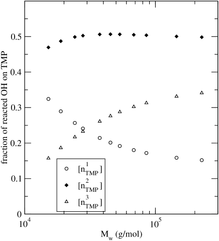
To reduce the number of free parameters further, we assume that the presence of one reacted OH group on a TMP molecule lowers the reaction rate by a certain fraction and the presence of two reacted OH groups inhibit the reaction rate of the third OH group independently ($k_{3}=k_{2}^{2}$). For a given acid concentration and value of $k_{2}/k_{1}$, the numerical solution of the rate equations yields the probabilities of having different reacted species in the final product (fig. 2). From these probabilities, we generate an ensemble of representative molecules by first selecting a species (PTMG, TMP_n or AD) with probabilities given by their respective weight fractions. Any unreacted acid group reacts with an OH group on either a PTMG molecule or a TMP_n molecule with the probabilities from the solution of eqn. 6. For TMP_n molecules, $n$ of the end groups are attached to AD molecules. For PTMG molecules, ends are attached to an acid group to have the probability of reacted OH groups on PTMG the same as that given by the solution of eqn. 6. Since the initial species is selected on a weight basis, in this way we generate a weight-biased molecular distribution and the probability weight of each individual molecule is simply the inverse of the total number of molecules so generated. For the rheological response, the molecules contribute with this probability weight. We have here assumed that there are no ring molecules and that the reactivities are independent of the size of the molecule - both of which assumptions are expected to break down as the gel point is approached. Also our analysis depends on the assumption of spatial homogeneity (continuously stirred reaction scheme).

III Static structure of branched PTMG polymers

Figure 3: Determining $M_{char}$ : the line represents the best fit $\phi(M)\sim M^{-3/2}exp(-M/M_{char})$ indicating the exponent $\tau=5/2$ and $M_{char}=2\times 10^{5}$ g/mol. $k_{2}/k_{1}$ is fixed to be $0.8$ in this plot.

For a given choice of $k_{2}/k_{1}$, the acid concentration $f_{a}$ is varied to generate a series of different $M_{W}$ ensembles. For mean-field gelation ensemble, the cut-off function in the molar mass distribution $f(M/M_{char})$ in eq. 1 is explicitly known to be rubinstein:colby

$$f(M/M_{char})=\exp\left[-\frac{M}{2M_{char}}\right].$$ (7)

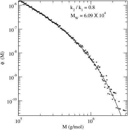
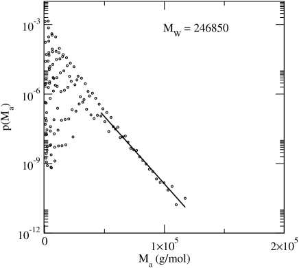
Using this cut-off function and assuming that the exponent $\tau=5/2$ in eqn. 1, we use a two-parameter fit to determine $M_{char}$ from the tail region of the molar mass distribution (fig. 3). Note that because our ensemble is generated on weight basis, we fit a function $\Phi(m)\sim M^{-3/2}\exp\left[-\frac{M}{2M_{char}}\right]$ corresponding to $\tau=5/2$. The small-mass end of the distribution (not shown in the figure) does not conform to this form and shows noisy features due to the finite size of the oligomers used during synthesis.

Figure 4: $M_{char}$ as a function of $M_{W}$ for several choices of $k_{2}/k_{1}$ ratios superposed with the experimental data.

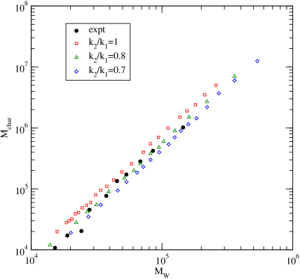
In fig. 4 we show $M_{char}$ as a function of $M_{W}$ for three different choices of $k_{2}/k_{1}$. For $k_{2}=k_{1}$, the simulation values of $M_{char}$ are consistently higher than the experimental points, while for $k_{2}=0.7k_{1}$, the simulation values are consistently lower. For $k_{2}=0.8k_{1}$, the simulation results closely match the experimental values.

Ref. lusignan:99 measured the intrinsic flow viscosity, $[\eta]$, and found a crossover from linear-like behavior ($[\eta]\sim M^{0.8}$) at low molar mass to randomly branched behavior ($[\eta]\sim M^{0.45}$) at high molar mass. When all the samples of different $M_{W}$ were considered together, the crossover of these two behaviors was found at $M_{X}=6.6\times 10^{4}$. Without knowledge of the detailed interaction among the monomers, it is not possible to compute the intrinsic viscosity. The intrinsic viscosity should depend linearly with the radius of gyration in a good solvent - which again is beyond our ability to calculate. However, it is reasonable to assume that the radius of gyration in a good solvent will be directly related to that in the $\Theta$ solution, and in particular that the crossover molar mass between the linear-like and the branched scaling will be the same. From the numerical ensemble of the polymers, we used Kramers theoremrubinstein:colby to calculate this ideal radius of gyration.

Figure 5: Ideal radius of gyration for $k_{2}=0.8k_{1}$ and $M_{W}=15200$ (filled circles) and $M_{W}=226000$ g/mol (open triangles). The line shows the combined behavior of all the data sets from samples with different $M_{W}$ together. $b$ is the Kuhn length and Kuhn mass is assumed to be $74$ g/mol.

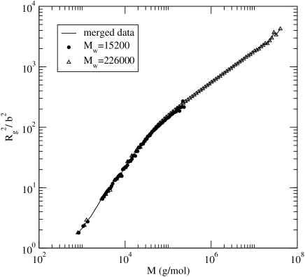
From the numerical ensemble of the molecules, we form histograms of molecules with respect to the mass of the molecules. For each bin in the histograms we calculate the average radius of gyration. For these calculations, we assume that the Kuhn mass is $74$ g/mol lusignan:99 and the results are in units of Kuhn length $b$. In fig. 5 we plot the radius of gyration for two different molar mass samples (symbols), both generated with $k_{2}/k_{1}=0.8$. Also shown is the radius of gyration when all the different molar mass samples are considered together (line). The individual $M_{W}$ ensembles roughly fall on this merged distribution line. A difference shows up only at the high molar mass limit - where the lower $M_{W}$ ensembles do not have any entries.

Figure 6: Crossover from linear to randomly branched behavior from radius of gyration. The symbols correspond to the radius of gyration determined by making a histogram in mass from all the different $M_{W}$ samples considered together. The solid line and the broken line corresponds to slopes $1$ (linear) and $1/2$ (randomly branched) respectively. The arrow indicates crossover at 65800 g/mol. $k_{2}/k_{1}$ is fixed at $0.8$.

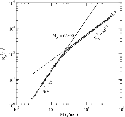
In fig. 6 we plot the radius of gyration when all samples are considered at $k_{2}=0.8k_{1}$. At the low-molar-mass end, the data fits the form $R_{g}^{2}\sim M$ corresponding to linear polymers. The high-molar-mass end fits the form $R_{g}^{2}\sim M^{1/2}$ corresponding to randomly branched polymers. The crossover of these two behaviors is found by extrapolating the fits at $M_{X}=65800$ g/mol. Increasing (decreasing) the value of $k_{2}$ leads to lowering (raising) $M_{X}$. For comparison, $k_{2}=1$ and $k_{2}=0.7$ respectively corresponds to $M_{X}=47500$ g/mol and $M_{X}=89000$ g/mol. Since the same value of $k_{2}/k_{1}$ fits both this crossover behavior and the variation of $M_{char}$ with $M_{W}$ with the experimental results, only results with this value of $k_{2}/k_{1}$ are shown in the rest of the paper. The quantitative agreement with quite different experimental results using the same parameter suggests that our simplistic assumptions about the reaction kinetics are probably close to reality.

Figure 7: Probability distribution of linear segments at a fixed acid concentration. $p(M_{N,S})$ decays exponentially at large $M_{N,S}$. The line denotes an exponential fit in the shown range.

From the cross-over in radius of gyration, one might conclude that the typical linear segment length is about 66000 g/mol (indeed, this is the conclusion in lusignan:99 from the intrinsic viscosity data). With the detailed topological connectivity at our disposal, we can probe the segment length between branch points in a different way. A linear segment can be made of PTMG oligomers connected by acid groups alone - or with intervening TMP molecules with only two of the three OH groups reacted. Such TMP connectors will have small side-arms (compared to entangled molecular mass) which will still behave as linear segments in rheological measurements. We therefore add the mass of such small side-arms to the backbone. This does not remove segments which are too small to be rheologically important but still are connected at all ends (for example, an H molecule with the cross bar formed by two TMP molecules will behave just like a four arm star). For this reason we take an alternative route than a simple average of the masses of the arms (we believe that this alternative route is also rheologically most relevant). Any random association to form linear segments attains a Flory distribution (most probable distribution) at mass scales much larger than the constituent elements. The probability of having a segment of length $M_{a}$ is given by $p(M_{a})=c\;\exp(-M/M_{N,S})$, with $c$ being an constant and, $M_{N,S}$ being the number-averaged molar mass of the segments. From a histogram of linear segments, we determine $p(M_{a}$ and using an exponential fit at large $M_{a}$ determine the number-averaged molar mass $M_{N,S}$ (fig. 7). The weight-averaged molar mass for Flory distribution is twice $M_{N,S}$.

Figure 8: Estimate of number averaged molar mass of linear segments between branch points as a function of $M_{W}$. The error bars are estimated from standard error in the exponential fit of $p(M_{a})$ (fig. 7).

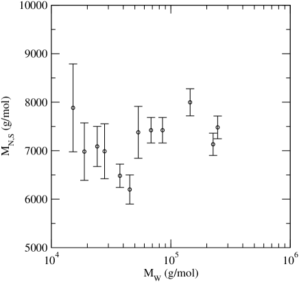
In fig 8 we plot $M_{N,S}$ as a function of $M_{W}$. The error bars correspond to the error estimates in exponential fit of $M(a)$ (fig. 7). determining the addition probability. At large $M_{W}$, the estimate of the linear segment length from this approach is $\sim 7200$ g/mol, which is almost an order smaller than $M_{X}$ determined from the crossover of radius of gyration. This is due to the fact that lightly branched material like stars or combs, which dominate the mid-range in the mass distribution, have a radius of gyration which is closer to that of linear polymers with the same molar mass than to that of randomly branched polymers.

Figure 9: Dependence of characteristic mass $M_{char}$ on the acid fraction $f_{a}$. The line is a linear fit for high $M_{W}$ samples. The intersection point with the zero x-axis gives the critical acid concentration $f_{a}^{c}$, where the characteristic mass diverges.

As an estimate for closeness to the gelation transition, we define

$$\epsilon\equiv\left(\frac{f_{a}^{c}-f_{a}}{f_{a}^{c}}\right),$$ (8)

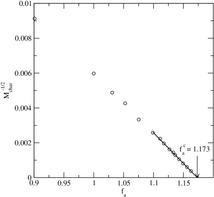
where, $f_{a}^{c}$ is the critical acid concentration where the characteristic mass diverges. Close to the gel point, the characteristic mass $M_{char}$ scales as $M_{char}\sim\epsilon^{-2}$. Thus the plot of $1/\sqrt{M_{char}}$ versus $f_{a}$ shows a linear behavior for large $f_{a}$ (fig. 9). The point at which the line crosses the zero x-axis (infinite $M_{char}$) determines $f_{a}^{c}=1.173(1)$. For $k_{2}/k_{1}=0.8$, the sample with average molar mass 220 Kg/mol corresponds to $f_{a}=1.156$ giving $\epsilon\sim 0.014$. The size of the largest branched molecule provides a characteristic length $\xi$ and mean-field theory provides a self-consistency test by requiring that the molecules of this characteristic size should overlap sufficiently. In 3 dimensions, this leads to a critical value of the extent of the reaction $\epsilon_{c}\sim N^{-1/3}$ below which the largest molecules no longer overlap significantly and the exponents change from the mean-field results degennes:77 ; lusignan:99 . Taking the linear segment length $M_{N,S}=7200$ g/mol and Kuhn mass to be $74$ g/mol, there are on average approximately 100 Kuhn segments between branch points. This estimate gives $\epsilon_{c}\simeq 100^{-1/3}\simeq 0.2$, so that the highest molar mass samples are much closer to the gelation transition than the critical value and are therefore expected to show non-mean-field behavior. We will meet the rheological consequences of this critical behavior in the following.

IV Rheological response of branched PTMG polymers

IV.1 Computational rheology

To estimate the rheological behavior of the entangled branched PTMG polymers, we employ a numerical approach larson:01 ; das:06 . For details, the reader is referred to das:06 . We summarize the procedure qualitatively here for completeness. The numerical approach is based on tube theory doi:book , which replaces the topological entanglements from neighboring chains by a hypothetical tube surrounding a given chain. After a small strain, the stress is relaxed by the escape of the chains from the old tube constraints. This connects the stress relaxation to the survival probability of the chains in their respective tubes. In a polymer melt, since all the polymers are in motion, the tube constraint itself is not fixed over time. This constraint release is handled by the dynamic dilation hypothesis marrucci:85 ; ball:89 ; colby:90 , which postulates a simple relation between the tube diameter and the amount of unrelaxed material. A free end monomer relaxes part of its tube constraint at short times by constraint-release Rouse motion. At later times, the entropic potential, which itself evolves due to constraint release, leads to a first-passage time approach milner:97 . The contribution from a collapsed side arm is modeled by including increased friction on the backbone, estimated from the time of collapse and the current tube diameter as a length-scale for diffusive hops from an Einstein relation. For branch-on-branch architectures, the relaxation leads to a multi-dimensional Kramers’ first-passage problem. We simplify this by recasting it to an effective one-dimensional problem which has the required Rouse scaling, respects topological connectivity and gives correct result at some special known limits das:06 . A linear or effectively linear (branched material with collapsed side arms) chain can relax by reptation. When a large amount of material relaxes quickly, such that the dynamically dilated tube increases in diameter faster than the rate permitted by Rouse relaxation, the effective orientational constraint responds more slowly by constraint release Rouse motion and the dynamic dilation is modified viovy:91 ; milner:98 . In addition, we include contributions from the Rouse motion inside the tube and fast forced redistribution of material at the early stages of the relaxation likhtman:02 .

In computational rheology, starting from a numerical ensemble of molecules, tube survival probability in discrete (logarithmic) time is followed after an imaginary step strain larson:01 ; park:05a ; park:05b ; das:06 . At each of these time steps, the amount of unrelaxed material $\phi_{t}$ and the effective amount of tube constraint $\phi_{ST}$ is stored. Since the visco-elastic polymers have a very broad spectrum of relaxation, we assume that the amount of material relaxed in each time step contribute as independent modes in the stress relaxation modulus $G(t)$. Thus after all of the molecules have relaxed completely, $G(t)$ is calculated as a sum over all these independent modes. The complex modulus $G^{*}(\omega)$ at frequency $\omega$ is defined by

$$G^{*}(\omega)=i\omega\int_{0}^{\infty}G(t)exp(-i\omega t)dt.$$ (9)

The real and imaginary parts of $G^{*}(\omega)$, storage modulus $G^{{}^{\prime}}(\omega)$ and the dissipative modulus $G^{{}^{\prime\prime}}(\omega)$ respectively, are of particular interest since they are measured in oscillatory shear experiments. The zero-shear viscosity $\eta$ is calculated from

$$\eta_{0}=\lim_{\omega\rightarrow 0}\frac{G^{{}^{\prime\prime}}(\omega)}{\omega},$$ (10)

and the steady-state compliance $J_{e}^{0}$ is calculated from

$$J_{e}^{0}=\lim_{\omega\rightarrow 0}\frac{G^{{}^{\prime}}}{(G^{{}^{\prime\prime}})^{2}}.$$ (11)

All the integrations are replaced by sums over discrete timesteps of the relaxation.

The calculations have a few free parameters. The material-dependent parameter of entanglement molar mass $M_{e}$ is related to the plateau modulus $G_{0}$ by larson:03

$$G_{0}\equiv\frac{4}{5}\frac{\rho RT}{M_{e}},$$ (12)

where, $\rho$ is the polymer density and $T$ is the temperature. The timescale is set by the entanglement time $\tau_{e}$ which is the Rouse time of the chain segment between entanglements. When the molar mass of the segments is scaled by $M_{e}$ and the time is scaled by $\tau_{e}$, in the approximation of tube theory, polymers of the same topology but of different chemical composition relax the same way. We assume that, for a side-arm relaxing completely at certain time $t_{a}$, at times much larger than $t_{a}$, the motion of the associated branch-point can be modeled as a simple diffusion process with hop size $pa$ at the timescale of $t_{a}$. Here $a$ is the tube diameter and $p$ is a numerical factor. We use $p^{2}=1/40$ as used in das:06 to fit a wide range of different experimental data. The dynamic dilation hypothesis assumes that the effective tube diameter depends on the amount of unrelaxed material and the effective number of entanglements associated with a segment of length Z scales as $Z\rightarrow\phi_{t}^{-\alpha}$. We choose the dynamic dilation exponent $\alpha=1$ in our calculations.

For the class of polymers considered in this study, the number of branches on a given molecule can be quite large. Also a large number of molecules need to be considered to ensure that a single massive molecule does not affect the results disproportionately. In our approximations, the relaxation of the different molecules are coupled only via the amount of unrelaxed material $\phi_{t}$. This enables us to divide the ensemble of molecules in several subsystems and follow the relaxation process independently at each step, communicating the local $\phi_{t}$ to other processors at the end of each time step. The minimal communication needed makes the parallel-code scale almost perfectly with the number of processors and most importantly allows us to probe closer to the gelation transition, where the memory requirement becomes larger than available on single processors. The source code, precompiled executables and documentation of the program are available from http://sourceforge.net/projects/bob-rheology.

IV.2 Dynamic exponents for branched PTMG

To calculate the dynamic properties of the branched PTMG molecules, we generated ensembles of $5\times 10^{5}$ molecules at each $M_{W}$ considered and followed the relaxation after a small step-strain. In the absence of high-frequency measurements for this material, we take $M_{e}$ and $\tau_{e}$ as free parameters - fitted to describe the dynamic properties. Without the complications of occasional ester groups from the esterification and the butyl side groups from the TMP molecules, the present polymers resemble polytetrahydrofuran (PTHF). For PTHF, treating it as an alternating copolymer of ethylene and ethylene oxide, the estimate of the entangled molecular weight is $M_{e}\simeq 1420$ g/mol fetters:pv . We use this value as our rough first guess for $M_{e}$ and fix $\tau_{e}$ by matching the zero-shear viscosity with experimental results at the intermediate molar mass range of the experimental data.

Figure 10: Zero-shear viscosity $\eta$ as a function of weight-average molar mass. Filled circles are the experimental data from lusignan:99 . The triangles and the squares are the results from our calculations using $M_{e}=1420$ and $1080$ g/mol respectively. The error bars for the $1080$ g/mol calculations represent the effect of uncertainty in $\eta$ corresponding to the experimental uncertainty of $10\%$ in determining $M_{W}$. The line is a power-law fit to the $M_{e}=1080$ g/mol results in the intermediate mass region with the exponent 3.95.

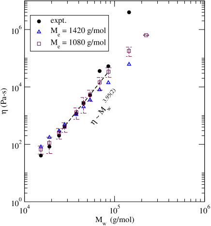
In fig. 10 we plot the zero shear viscosity $\eta$ for different values of $M_{W}$. The filled circles are the experimental results from lusignan:99 . The triangles are results from our calculations with $M_{e}=1420$ g/mol and $\tau_{e}=1.8e-7$ s. For this choice of $M_{e}$, the viscosity increases slowly with $M_{W}$ compared to the experimental data. The squares are results with $M_{e}=1080$ g/mol and $\tau_{e}=3.45e-8$ s. This choice of $M_{e}$ is able to reproduce the experimental viscosity data over half a decade in $M_{W}$. A power-law fit in the intermediate range (shown as a dashed line in the figure) gives the viscosity exponent $s=3.95(2)$. In the experiments, there is an uncertainty of $10\%$ in determining $M_{W}$. The error bars in the $M_{e}=1080$ g/mol data show the associated uncertainty in viscosity. At the largest $M_{W}$, our calculations and the experimental data show opposite trends. The viscosity from our calculations shows a trend of lowering of the exponent at the largest $M_{W}$, while the experimental data shows a sharp increase. For rest of the results in this section, we use $M_{e}=1080$ g/mol.

Figure 11: Complex viscosity $\eta^{*}(\omega)$ for selected $M_{W}$. Lines are from calculations in this study, symbols are experimental data from lusignan:99 .

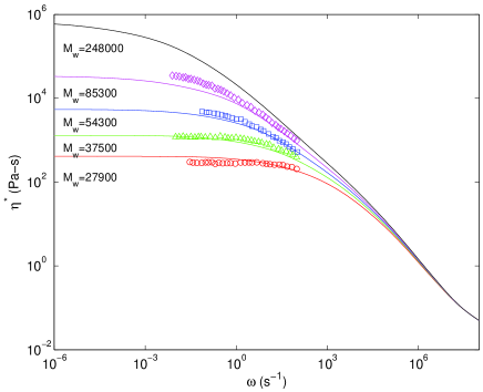
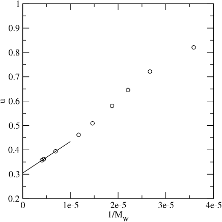
Fig. 11 shows the frequency dependence of the complex viscosity $\eta^{*}(\omega)$ for several different values of $M_{W}$. Symbols represent experimental data from lusignan:99 in the intermediate mass range, where zero-shear viscosity from our calculation matches with the experimental values. $\eta^{*}(\omega)$ shows an approximate power-law behavior with exponent $1-u$. Away from the gelation transition, this power-law window is limited. We fitted power laws in the frequency range 10-100 s^-1 to estimate the exponent. Since $1/M_{W}\sim\epsilon$, we plotted $u(M_{W})$ from such fitting as a function of $1/M_{W}$ (fig. 12). Linear extrapolation to $1/M_{W}\rightarrow 0$ gives the limiting value of $u=0.305(1)$, which corresponds closely to the experimental value of $u=0.31(2)$.

Figure 12: Variation of the relaxation exponent $u$ with $M_{W}$. The line shows the extrapolation used for large $M_{W}$ to find the value of $u$ at the gel transition.

V Mean-field gelation ensemble

The segment length for branched PTMG considered in the earlier part of the paper is largely determined by the size of the oligomer used to synthesize the polymers. In this section we turn to a hypothetical series of polymers which fall in the category of mean-field gelation class. We consider linear molecules of type $A$ which are Flory distributed and tri-functional groups $B$ which have zero mass. The molecules are formed by the rule that $A$ reacts with $B$ and neither $A$-$A$ nor $B$-$B$ reactions are allowed. Furthermore, we assume that, at the end of the reaction, all $B$ bonds are attached to some $A$ molecules. Thus, as in the case of branched PTMG polymers, extent of the reaction is determined by stoichiometric mismatch. As before, we assume that there are no closed loops. The final distribution of the molecules are described by only two parameters: $M_{N,S}$, number-averaged molar mass of the linear segments and $p_{b}$, the branching probability. The molecules are generated by selecting the first strand with a Flory distribution of length $M_{N,S}$ and adding Flory distributed branches recursively on both ends with probability $p_{b}$.

The static properties of these molecules can be solved analytically. The characteristic molar mass diverges when $p_{b}$ is 0.5 ($\epsilon\equiv(0.5-p_{b})/0.5$). Using seniority variables to approximately describe the hierarchical relaxation, ref. read:01 found that the entangled contribution to the terminal relaxation time of this class of polymers does not diverge at the percolation threshold. Their calculation did not include the constraint release Rouse modes, contributions from which will still be divergent in the absence of a diverging entangled contribution. For the calculations presented in this section, we assume $M_{e}=1120$ g/mol and $\tau_{e}=1.05\times 10^{-8}$ s, corresponding to high-density polyethylene at 150^o C das:06 . For each value of $p_{b}$ and $M_{N,S}$ considered, we generate an ensemble of $2\times 10^{5}$ molecules and follow the relaxation after a step strain. To estimate statistical errors involved in our calculations, for each case we repeat the calculation 3 times with different sets of molecules (generated by different random seeds).

Figure 13: Radius of gyration for gelation ensemble with $M_{N,S}=22400$ g/mol with $p_{b}=0.49$. The cross-over mass $M_{X}=314400$ is roughly 14 times larger than $M_{N,S}$.

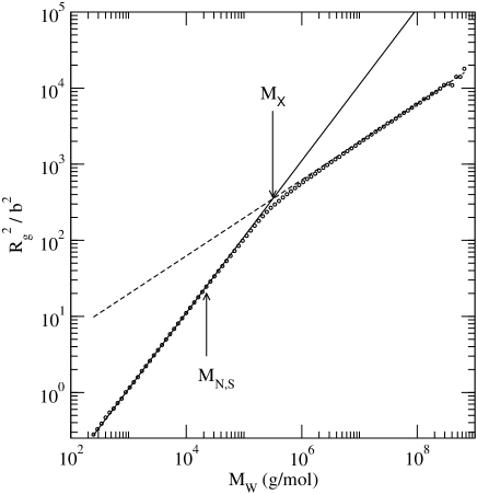
In fig. 13 we plot the mass dependence of the radius of gyration for $p_{b}=0.490$ ($\epsilon=0.02$) and segment length $M_{N,S}=22400$ g/mol (number of entanglements between branch points $N/N_{e}=20$). As in the case of branched PTMG, the extrapolated cross-over mass $M_{X}$ in radius of gyration from linear to the randomly branched behavior is much larger than $M_{N,S}$. Because the segments are Flory distributed with out a lower cutoff, the difference is even larger in this case ($M_{X}/M_{N,S}\sim 14$).

Figure 14: Estimating the exponent u : the left panel shows $\eta^{*}(\omega)$ for $N/N_{e}=20$ and $\epsilon=0.4$, $0.2$, and $0.02$. Data for different $\epsilon$ are fitted separately to a power law with exponent $1-u$ in the frequency range $10^{2}-10^{4}$ s^-1. The exponent $u$ so obtained, as a function of $\epsilon$, is plotted in the right panel. A linear fit for $\epsilon\leq 0.1$ was used to find the limiting value of $u$ at this $N/N_{e}$.

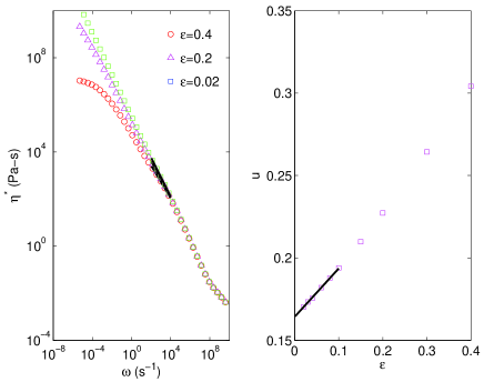
Fig. 14 illustrates the procedure followed for estimating the apparent relaxation exponent $u$ (when the relaxation dynamics are entangled there is no reason to expect true power-law behavior, but an apparent power law can hold as a good approximation for a sizeable range of relaxation timescales rubinstein:90 ). The left subpanel shows the variation of the complex viscosity $\eta^{*}$ with frequency for three different $\epsilon$ for $N/N_{e}=20$. At the lowest frequencies, for $\epsilon=0.4$, the terminal relaxation leads to significant deviation from the power-law behavior. For smaller values of $\epsilon$, this deviation shifts to smaller frequencies. For different $\epsilon$, we fit a power law with exponent $1-u$ in the frequency range $10^{2}-10^{4}$ s^-1. In the right subpanel of fig. 14 we plot the dependence of such apparent $u$ with $\epsilon$. For $\epsilon\leq 0.1$, the values of $u$ shows a linear dependence on $\epsilon$. A linear fit was used to estimate the extrapolated value of $u$ at $\epsilon=0$.

Figure 15: Variation of (apparent) relaxation exponent $u$ with $N/N_{e}$. The circles are the data obtained from our calculations. The dotted line is the prediction of hierarchical relaxation model of rubinstein:90 and the dashed line is the phenomenological form used in lusignan:99 . The triangle corresponds to the exponent $u$ for the branched PTMG polymers, when the segment length is estimated by fitting a Flory distribution to the probability distribution of segment lengths.

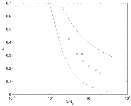
Fig. 15 shows the extrapolated values of $u$ (circles) at $\epsilon=0$ from the procedure outlined in fig. 14 as a function of number of entanglements between branch points $N/N_{e}$. The error estimates for $u$ are smaller than the size of the symbols. An approximate calculation of hierarchical relaxation in entangled mean-field gelation tube model at the gel point rubinstein:90 predicted a form of $u$ as

$$u=\psi\frac{N_{e}}{N}\;\;\;{\text{for}}\;\;N\geq N_{e},$$ (13)

with $\psi$ being a constant. Both theory and experiments for $N<N_{e}$, where unentangled Rouse dynamics dominate, suggest $\psi\approx 0.67$. The dotted line shows the prediction from eqn. 13. Ref. lusignan:99 uses an empirical function,

$$u=\left\{\begin{aligned} &0.67&N<2N_{e}\\ &\frac{3}{3+2\ln(N/N_{e})}\;\;&N>2N_{e},\end{aligned}\right.$$ (14)

to describe the dependence of $u$ on $N/N_{e}$ from experimental data. The dashed line in fig. 15 shows this phenomenological function. Results from our calculations fall roughly midway between the prediction of the approximate model rubinstein:90 and the phenomenological fit to data in lusignan:99 . The significant deviation from eq. 14 is mostly because lusignan:99 uses $M_{X}$ as an indicator for $M_{N,S}$ (so overestimating it) and to some extent because $u$ changes appreciably as the limit $\epsilon\rightarrow 0$ is considered (fig. 14). When plotted against our estimate of linear segment length (shown as triangle in fig. 14), the exponent $u$ corresponding to the experiments reported in ref. lusignan:99 matches closely with our calculations on gelation ensemble.

Figure 16: Zero-shear viscosity $\eta$ and recoverable compliance $J_{e}^{0}$ as a function of $\epsilon$ for different $N/N_{e}$. The left subplot shows $\eta$ for $N/N_{e}=3$, $5$, $7$, $10$, and $20$. The right subplot shows $J_{e}^{0}$ for only $N/N_{e}\geq 7$.

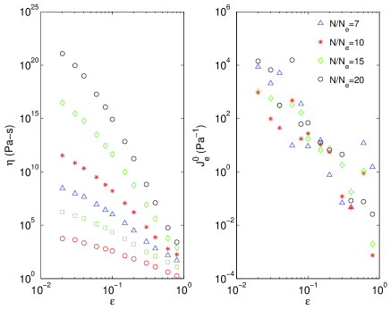
The left subpanel of fig. 16 shows the zero-shear viscosity $\eta$ as a function of $\epsilon$ for different value of $N/N_{e}$ (larger $N/N_{e}$ data have higher viscosity at the same $\epsilon$). The right subpanel shows the recoverable compliance $J_{e}^{0}$ for $N/N_{e}=7$, $10$, $15$, and $20$. The data shows a large amount of scatter. $J_{e}^{0}$ can be expressed as the first moment of $G(t)$ : $J_{e}^{0}=\left(\int_{0}^{\infty}tG(t)dt\right)/\eta^{2}$. Thus, $J_{e}^{0}$ is particularly susceptible to the long-time decay of $G(t)$. The longest relaxation time is dominated by just a few of the high molar mass molecules in our ensemble. Thus the variation of $J_{e}^{0}$ with the particular ensemble considered is large. For small $N/N_{e}$, the relative contribution from this tail region of molar mass distribution is even higher. For $N/N_{e}<7$, the scatter becomes larger than the value of $J_{e}^{0}$ and they are neither shown in the figure nor considered for further analysis.

Figure 17: Viscosity exponent $s$ as a function of $N/N_{e}$. The circles are results from our calculations and the dashed line is the phenomenological form of Lusignan et al. lusignan:99 .

At the smallest values of $\epsilon$ plotted in the log-log plot in fig 16, in double log plot, the slope of $\eta$ with $\epsilon$ starts to decrease. To probe at even smaller $\epsilon$ would require much larger computations than used in this study. Instead we focus our attention in the range of $\epsilon$ between $0.006$ and $0.2$, where the viscosity for all values of $N/N_{e}$ shows approximate power-law dependence on $\epsilon$. Fig. 17 shows the viscosity exponent $s$ as a function of $N/N_{e}$. Also shown is the phenomenological form of lusignan:99 as dashed line

$$s=\left\{\begin{aligned} &1.33&N<2N_{e}\\ &2\ln(N/N_{e})\;\;&N>2N_{e}.\end{aligned}\right.$$ (15)

Results from our calculations show a much sharper increase of $s$ with $N/N_{e}$ than predicted by this functional form.

Figure 18: Recoverable compliance exponent t as a function of $N/N_{e}$. The circles represent results from a direct power-law fit of the form $J_{e}^{0}\sim\epsilon^{-t}$. The error bars are estimated from the variance in $J_{e}^{0}$ from three independent sets of molecular ensemble. The squares are calculated by using the hyperscaling relationship (eq. 16). For $N/N_{e}=3$ and $5$, the scatter in $J_{e}^{0}$ is too large for a direct estimate of $t$.

In fig. 18, we plot the recoverable compliance exponent $t$ (circles) as a function of $N/N_{e}$. Because of large scatter in $J_{e}^{0}$, the error estimates in this case are large (error bars are estimates of error from the variance obtained from three independent sets of calculations). Since both $\eta$ and $J_{e}^{0}$ can be expressed as integrals over $G(t)$, the exponents $u$, $s$ and $t$ are not independent. If $G(t)$ behaves like $t^{-u}$ till the longest relaxation time, one gets a dynamic hyperscaling relationship among the exponents

$$u=\frac{t}{s+t}.$$ (16)

The estimates of $t$ from estimates of $u$ and $s$ using this hyperscaling relation is shown as the squares in fig. 18. In the range of $N/N_{e}$, where we have direct estimates of $t$, estimates from the hyperscaling relationship falls below the direct estimate.

Figure 19: G(t) (symbols) for $N/N_{e}=3$ for $\epsilon=0.1$, $0.08$, $0.06$, $0.04$ and $0.02$. As $\epsilon$ is made smaller, $G(t)$ decays slowly. The vertical dotted lines show the range in which the complex viscosity is fitted (in frequency) to find the value of the exponent $u$. The solid line represents this limiting power law decay $G(t)\sim t^{-u}$ with the indicated slope $u=0.4253$.

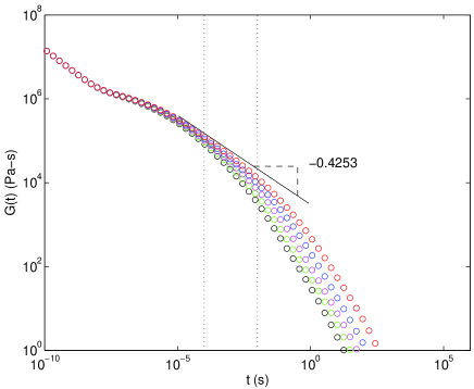
To explore why this is so, in fig. 19 we plot the decay of $G(t)$ for different values of $\epsilon$ and $N/N_{e}=3$. Also shown is the limiting power law decay suggested from fitting the complex viscosity data. For even the lowest $\epsilon$ studied here, the power-law behavior holds in only a small window of the relaxation time and the contribution in $\eta$ or $J_{e}^{0}$ from decay at times larger than this power-law window is not negligible. Thus, the dynamic hyperscaling relationship holds only approximately (fig. 18).

VI Conclusions

We have presented a simple kinetic modeling scheme for the gelation ensemble polymer synthesis in lusignan:99 . With just one global fitting parameter describing the branching chemistry, we are able quantitatively to reproduce the variation of characteristic molar mass $M_{char}$ as a function of $M_{W}$ and the behavior of intrinsic viscosity as a function of molar mass. With the detailed knowledge of the molecular topology in our calculations, our estimate of the average segment length between branch-points is much lower than estimated in lusignan:99 . We have used a numerical technique based on the tube theory of polymer melts to calculate the dynamic response of the polymers in the linear response regime. For intermediate ranges of $M_{W}$, both the complex viscosity $\eta^{*}(\omega)$ and the zero-shear viscosity $\eta$ matches with the experimental findings. For the largest $M_{W}$ considered, $\eta$ in our calculations is significantly lower than the experimental data. At those $M_{W}$, our estimate of closeness to the gelation transition $\epsilon$ is well below the Ginzburg-de Gennes criterion degennes:77 which is a feature of the highest $M_{W}$ polymers that distinguishes them from the others in the set. Hence the difference is likely to be due to non-mean-field behavior of these samples. Also, the four highest molar mass samples were prepared under slightly different conditions - where a partial reaction was carried out with stirring and, for the later part, the samples were reacted without stirring at a slightly elevated temperature lusignan:99 . Thus, our assumption of continuous stirred reaction may not be completely true for these samples. The dynamic exponents calculated from our calculations match with the experimental findings in the relevant $M_{W}$ range.

To investigate the behavior of the dynamic exponents with average segmental lengths between branch points, we calculated the relaxation properties of a series of molecules in the ideal mean-field gelation ensemble. The dependence of the relaxation exponent $u$ on $N/N_{e}$ falls about midway between the prediction of rubinstein:90 and the phenomenological form of lusignan:99 . We find that the viscosity exponent becomes smaller as $\epsilon$ is lowered. This is due to the dominance of supertube Rouse relaxation at long time scales for this class of polymers and, for small enough $\epsilon$, the viscosity exponent for any $N/N_{e}$ approaches the Rouse value applicable to the unentangled polymers.

The recoverable compliance exponent $t$ in our calculations have values similar to those found in experiments. It is worth noting, however, that the magnitude of $J_{e}^{0}$, when calculated from our algorithm, is found to be much larger than experimental values on similarly branched systems. Being the first moment of the relaxation modulus $G(t)$, the dominant contribution to $J_{e}^{0}$ comes from the long time behavior of $G(t)$, so is very sensitive to the assumptions on which the relaxation dynamics of the very largest clusters in the ensemble is based. The computational scheme we used to follow the relaxation in the melt extrapolates ideas of dynamic dilation and supertube relaxation which originally were formulated for linear or lightly branched systems to a highly branched system. In particular it assumes that the final supertube relaxation follows a Rouse scaling corresponding to a linear object. The final relaxation, provided that the tail of the distribution is long enough, of largely unentangled high molar mass molecules may find a faster route by showing a Zimm like relaxation, by which the largest clusters relax hydrodynamically in an effective solvent provided by the smaller clusters. In linear systems the transition molecular weight for this is the same as that for incomplete static screening of the larger molecules’ self-interactions. Experimental results on model systems with high seniority and well characterized branching and molar mass are needed to quantitatively test the validity of the theory for accounting the long-time decay of stress in such highly branched systems.

In summary, a numerical calculation of the entangled rheology of a series of mean-field gelation ensemble polymers provide a remarkable support of the accuracy of the hierarchical relaxation process suggested by the tube model.

References

- (1) C. P. Lusignan, T. H. Mourey, J. C. Wilson, and R. H. Colby, Phys. Rev. E 60, 5657 (1999).
- (2) C. Das, N. J. Inkson, D. J. Read, M. A. Kelmanson, and T. C. B. McLeish, J. Rheol., 50, 207 (2006).
- (3) D. Stauffer and A. Aharony, Introduction to Percolation Theroy, 2nd ed. (Taylor and Francis, London, 1992).
- (4) P. G. de Gennes, Scaling Concepts in Polymer Physics (Cornell University Press, Ithaca, 1979).
- (5) M. Rubinstein and R. H. Colby, Polymer Physics, (Oxford University Press, Oxford, 2003).
- (6) W. H. Stockmayer, J. Chem. Phys. 11, 45 (1943).
- (7) P. J. Flory, Principles of Polymer Chemistry (Cornell University Press, Ithaca, 1953).
- (8) J. Alder, Y. Meir, A. Aharony, and A. B. Harris, Phys. Rev. E 41, 9183 (1990).
- (9) E. M. Valles and C. W. Macosko, Macromolecules 12, 521 (1979).
- (10) D. Stauffer, A. Coniglio, and M. Adam, Adv. Polym. Sci. 44, 103 (1983).
- (11) D. Durand, M. Delsanti, M. Adam, and J. M. Luck, Europhys. Lett. 3, 297 (1987).
- (12) H. H. Winter, Prog. Colloid Polym. Sci. 75, 104 (1987).
- (13) J. E. Martin, D. A. Adolf, and J. P. Wilcoxon, Phys. Rev. A 39, 1325 (1989).
- (14) E. Nicol, T. Nicolai, and D. Durand, Macromolecules, 34, 5205 (2001).
- (15) E. Gasilova, L. Benyahia, D. Durand, and T. Nicolai, Macromolecules, 35, 141 (2002).
- (16) M. E. Cates, J. Phys. France 46, 1059 (1985).
- (17) M. Rubinstein, S. Zurek, T. C. B. McLeish, and R. C. Ball, J. Phys. France 51, 757 (1990).
- (18) M. Doi, and S. F. Edwards, The Theory of Polymer Dynamics (Claredon Press, Oxford, U.K., 1986).
- (19) G. Marrucci, J. Polym. Sci., Polym. Phys. Ed. 23, 159 (1985).
- (20) R. C. Ball, and T. C. B. McLeish, Macromolecules 22, 1911 (1989).
- (21) R. H. Colby, and M. Rubinstein, Macromolecules 23, 2753 (1990).
- (22) J. L. Viovy, M. Rubinstein and R. H. Colby, Macromolecules 24, 3587 (1991).
- (23) S. T. Milner, T. C. B. McLeish, R. N. Young, A. Hakiki, and J. M. Johnson, Macromolecules, 31, 9345 (1998).
- (24) P. G. de Gennes, J. Phys. (Paris) Lett. 38L, 355 (1977).
- (25) R. G. Larson, Macromolecules 34, 4556 (2001).
- (26) S. T. Milner and T. C. B. McLeish, Macromolecules, 30, 2159 (1997).
- (27) A. E. Likhtman and T. C. B. McLeish, Macromolecules, 35, 6332, (2002).
- (28) S. J. Park, S. Shanbhag and R. G. Larson, Rheol. Acta, 44, 319 (2005).
- (29) S. J. Park and R G Larson, J. Rheol., 49, 523 (2005).
- (30) R. G. Larson, T. Sridhar, L. G. Leal, G. H. McKinley, A. E. Likhtman, and T. C. B. McLeish, J. Rheol., 47, 809 (2003).
- (31) L. J. Fetters, private communication.
- (32) D. J. Read, and T. C. B. McLeish, Macromolecules 34, 1928 (2001).