Transport through the intertube links between two parallel carbon nanotubes

Abstract

Quantum transport through the junction between two metallic carbon nanotubes connected by intertube links has been studied within the TB method and Landauer formula. It is found that the conductance oscillates with both of the coupling strength and length. The corresponding local density of states (LDOS) is clearly shown and can be used to explain the reason why there are such kinds of oscillations of the conductances, which should be noted in the design of nanotube-based devices.

I Introduction

Since the discovery of single-walled carbon nanotube (SWNT) by Iijima,Iijima it had inspired great interests during the past years, due to its unique structural and electronic qualities Dresselhaus and great potential applications for nanodevices. Many prototypes of electronic devices based on carbon nanotubes have been realized in experiments, such as field-effect transistors,device1 single-electron transistors,device2 rectifiers,device3 nonvolatile random access memorydevice4 and so on. SWNT can be metallic or semiconducting depending on its diameter and helicity. Because of the small size in diameter, transport through carbon nanotubes is in ballistic regime. A perfect metallic SWNT has two crossing energy bands near the Fermi level ($E_{F}$), namely, the $\pi$-bonding and $\pi$-antibonding bands. These two bands act as conducting channels and contribute two conductance quanta to the low bias conductance $G(=2G_{0}=4e^{2}/h)$ according to the Landauer formula.Datta

Many efforts have been made to manipulate the electronic properties of carbon nanotubes, such as doping, deforming Yu ,functionalization,Strano and construction of various structures consisting of nanotubes. Interface or junction becomes a critical issue for mesoscopic transport in many cases. In the previous researches, carbon nanotubes have demonstrated quite different properties, such as ballistic transportballistic , Coulomb blockadeqd and Luttinger liquid behaviorsll . It is the contact effects and the inner scattering mechanisms that play the key role and make the nanotubes fall into different regimes. The influence of interface between SWNT and metal electrode on the conductance has been studied both in the frame of TB modelXue and ab initio calculation.Taylor These results showed that the interface affected the transport strongly.

The junctions of carbon nanotubes, such as cross, Y and T shapes, have been studied experimentally and theoretically, and showed unusual physical properties. Two carbon nanotubes with different diameters can be linked by pentagon and heptagon pairs in the junction.Dresselhaus The stable junctions of various geometries have been fabricated with the help of transmission electron microscope in experiments.Terrones Molecular dynamics calculations were implemented to simulate the bombardment of nanotubes and demonstrated that the crossed nanotubes could be welded.Krasheninnikov Under pressure, the intertube links are formed between the zigzag nanotubes in the SWNT ropes. Meanwhile, it was pointed that similar interlinking C-C bonds do not form between the (6, 6) parallel tubes even if they were deformed under a very high pressure.Yildirim

The study of the transport through these nanotube junctions is an important subject. It have been showed that intertube conductance through the junctions of two crossed single-walled carbon nanotubes was strongly dependent on the atomic registries between the two tubes.Fuhrer A significant conductance is allowed through the junction under relatively weak contact forces. These interlinking bonds survive even after the contact forces are released and the whole structure is fully relaxed.Buldum As for two parallel SWNTs, it is expected that they are linked by the van der Waals interaction when their distance is larger than $D_{vdW}=s_{vdW}+2R$,($s_{vdW}\sim$ 3.3 Å, R is the radius of the nanotube). By constraining them with the distance $D<D_{vdW}$, the interlinking bonds are easily formed between two tubes. The results of calculation indicated that the junction provided good transport in some atomic registries.Dag

How the coupling strength and length affect the transport through the intertube links between two parallel nanotubes? This is an interesting and valuable question because it is one of requisite steps to realize the pure-nanotube based devices. However, these effects have not been investigated systematically so far. Here the TB method is taken to deal with the junction of the parallel nanotubes and these effects are explored within the Landauer formula. The configuration is taken as that the coupling part of the two parallel metallic zigzag nanotubes is placed symmetrically and two atoms are connected in each unit cell (u.c.).

II Model and Formula

The $\pi$-electron tight-binding (TB) model and the Green’s function method have been used to accomplish the calculation. It is proved to be valid for states near the $E_{F}$ by previous ab initio calculations.Rubio According to the band structure calculations, the states crossing the $E_{F}$ are predominantly $\pi$ like in character. The electronic and transport properties of carbon nanotubes should be dominated by $\pi$ electrons. It can provide satisfied results to use the nearest-neighboring tight-binding model with one $\pi$ electron per carbon atom.song In our calculations, on-site energies are set to zero and all the hopping parameters between nearest sites equal to 2.66 eV.Chico

In our model, we take the configuration containing two parallel open ended SWNTs. In figure 1(a), the geometric scheme of the junction is given. The two nanotubes are linked by the bonds formed between two nearest C atoms in each unit cell. Figure 1(b) gives the view from one end along the axis. We can see that two nearest atoms are connected by the intertube link, which is both mechanical and electronic. Once the coupling part is included, the length of nanotubes chosen as conductor has no effect on the results for certain numbers of coupling unit cells. We only take the coupling part as conductor in our calculations, and take the nanotubes beyond the conductor part as leads, as shown in figure 1(c). Each nanotube is kept regular shape because the deformation is small and the effects of deformation on transport can be neglected. As mentioned earlier, we take $\pi$-electron tight-binding model to deal with the junction, which contributes the main part of conductance. The link is covalent $\sigma$ like bond formed between two opposite $\pi$ electrons and the coupling strength $t_{c}$ is taken to describe the link between them.

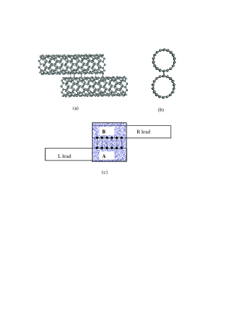
Figure 1: Schematic geometry of the junction. (a) Two nanotubes connected by intertube link. (b) View along the axis from one end. (c) The structure is divided as L(left) lead, conductor and R(right) lead to implement the calculation.

It should be mentioned, as some theoretical researches pointed, isolated primary metallic SWNTs except the armchair SWNTs generate a pseudogap near the $E_{F}$ due to the curvature. (6,0) carbon nanotube is always metallic, the other (3I,0) zigzag nanobubes (I is a integer), have a minigap which is on the order of $10^{-1}$ eV, and the magnitude is depend inversely on the square of tube radius gulseren ; zolyomi ; ouyang . The gap is so small that the bias voltage which need not very high can strike the gap to realize transport. It can be smeared by the small thermal fluctuation at finite temperature also. As many previous researches, here we do not consider the curvature effect in the TB model either.

Within the Landauer formalism, the conductance $G(E)$ of the system can be calculated as a function of the energy E of incident channels from the lead:

$$G(E)=G_{0}Tr[{\Gamma_{R}}{G^{r}_{c}}\Gamma_{L}{G^{a}_{c}}]$$ (1)

where $\Gamma_{L(R)}$ is the coupling matrix between the left (right) lead and the conductor, and $G^{r}_{c}$ is the retarded Green’s function which can be written as

$$G^{r}_{c}=(E-H_{c}-\Sigma_{L}-\Sigma_{R})^{-1},G^{a}_{c}=G^{r+}_{c}$$ (2)

Here $H_{c}$ is the Hamiltonian matrix of the conductor that represents the interaction between the atoms in the conductor, and $\Sigma_{L(R)}$ is the self-energy function that describes the effect of the left (right) lead. Once $\Sigma_{L(R)}$ is known, $\Gamma_{L(R)}$ is easily obtained as

$$\Gamma_{L}=i(\Sigma_{L}-\Sigma^{+}_{L}),\Gamma_{R}=i(\Sigma_{R}-\Sigma^{+}_{R})$$ (3)

$\Sigma_{L}(R)$ can be computed along the lines of Ref. 30 by using the surface Green s function matching theory. $\Sigma_{L}=H^{+}_{LC}\textbf{\emph{g}}_{L}{H_{LC}},\Sigma_{R}=H_{CR}\textbf{\emph{g}}_{R}{H^{+}_{CR}}$. $\textbf{\emph{g}}_{L(R)}$ is Green’s function for semi-infinite lead, and can be calculated through transfer matrices T and $\bar{T}$.

$$\textbf{\emph{g}}_{L}=({E-H_{00}-H^{+}_{01}{\bar{T}}})^{-1},\textbf{\emph{g}}_{R}=({E-H_{00}-H_{01}T})^{-1}$$ (4)

Transfer matrices T and $\bar{T}$ can be easily computed via an iterative procedure.

Once $G^{r}_{c}$ are known, the total density of states (DOS) can be easily computed,

$$\rho=-Im[Tr({G^{r}_{c}})]/\pi$$ (5)

We can calculate the Local density of states (LDOS) for the $j_{th}$ site in the conductor from the diagonal elements of $G^{r}_{c}$,

$$\rho_{j}=-Im[(G^{r}_{c})_{j,j}]/\pi$$ (6)

In the case of transport through the interface between A and B, $H_{c}$ and $G^{R}_{c}$ can be writen

$$H_{c}=\left(\begin{array}[]{ccc}H_{AA}&H_{AB}\\ H_{BA}&H_{BB}\end{array}\right),G^{r}_{c}=\left(\begin{array}[]{ccc}G_{AA}&G_{AB}\\ G_{BA}&G_{BB}\end{array}\right)$$

and the conductance can be written asNardelli

$$G(E)=G_{0}Tr[{\Gamma_{A}}{G^{r}_{AB}}\Gamma_{B}{G^{a}_{BA}}].$$ (7)

III Results and Discussion

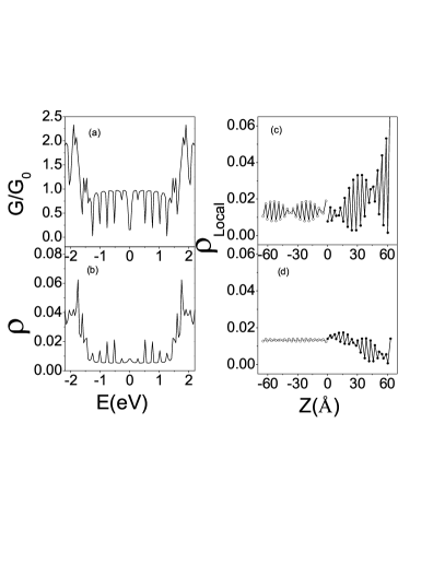
Figure 2: Quantum conductance G (a) and the corresponding total density of states (b) as a function of energy E for (9,0)-(9,0) SWNT with 15 coupling u.c. The local density of states of the sites in the coupling line for E=-0.272eV, G=0.77$G_{0}$ (c) and E=-0.223eV, G=0.97$G_{0}$ (d) are plotted.

The links of C atoms between the two parallel nanotubes provide a channel for the transport, but its value is limited to not above the unit of quantum conductance near the $E_{F}$ due to the scattering mechanism. Electrons in the two nanotubes interfere through the interactions between them, and become extended or localized in these links. The transport through the junction can be tuned by the coupling strength and length. In order to explore the inner mechanism, we have calculated the LDOS of the sites in the coupling line.

Fig 2(a) and 2(b) show the quantum conductance and the corresponding DOS for 15 coupling unit cells respectively. There are many peaks in the DOS, and the corresponding valleys of conductance appear at the same energy. These peaks in the DOS are local peaks which give rise to the valleys of conductance function. With longer coupling length, the peaks in the DOS and valleys in conductance are much more complicated. The conductance at certain energy or the average value near $E_{F}$ experiences oscillations with the coupling length increasing, which will be illustrated later. Fig 2(c) is the LDOS at E=-0.273eV and the corresponding $G=0.77G_{0}$, which is a valley in the conductance function, and we find that the density fluctuations are strong. On the contrary, the LDOS at E=-0.223eV has weak fluctuations in the conductor part, and the corresponding conductance reaches a high value, $G=0.97G_{0}$.

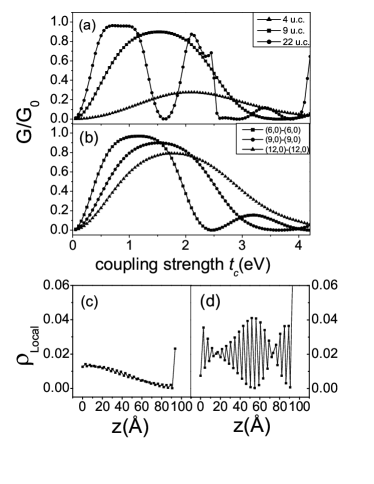
Figure 3: (a) Conductance at E=-0.13eV versus coupling strength for (9,0)-(9,0) SWNT with 4 (triangle), 9 (square) and 22 (circle) coupling u.c. respectively. (b) Conductance versus coupling strength for the configuration of (6,0)-(6,0)(triangle), (9,0)-(9,0) (square) and (12,0)-(12,0) (circle) SWNT with 9 coupling u.c respectively. (c) The LDOS of sites in coupling line of the nanotubes, with coupling strength $t_{c}=0.8eV$. (d) The LDOS with coupling strength $t_{c}=1.6eV$.

Considering the pseudogap in the zigzag carbon nanotube due to its curvature, which is not included in our model, we take the incident energy near the $E_{F}$ but outside the small gap. We investigate the dependence of the conductance on the coupling strength at E=-0.13eV for two (9,0) metallic zigzag nanotubes. The conductance undergoes damped oscillations, and reaches almost zero after a few oscillations as illustrated in figure 3(a) for different coupling strength. This oscillating phenomena is very similar with the recent results in the experiment for the squashed carbon nanotubes,Navarro where the conductance oscillations are caused by the open-close cycles of gap due to deformation. Here the oscillations have different origin, and are caused by delocalization and localization due to the effective deformation induced by intertube link. The effective deformation does not produce the gap, but causes localization and delocalization, and then affects the transport channel between the two nanotubes. In figure 3(a), the conductance is plotted as the function of coupling strength for 9, 14 and 22 u.c. respectively. We can see that the conductance is more sensitive to the coupling strength and experiences more oscillations before getting blocked if the coupling length is longer. In figure 3(b), the conduction versus coupling strength is given for three different configurations. If the coupling length is fixed, it needs higher coupling strength to reach the first maximum of conduction for the two nanotubes with bigger radii and the corresponding maximum value is smaller. Figure 3(c) and 3(d) give the LDOS of the sites in the coupling line for $t_{c}=0.8eV$ and $t_{c}=1.6eV$ and the corresponding conductance are 0.96$G_{0}$ and 0.003$G_{0}$ respectively. We can see from the figure that the LDOS fluctuations are weak when the conductance is high.

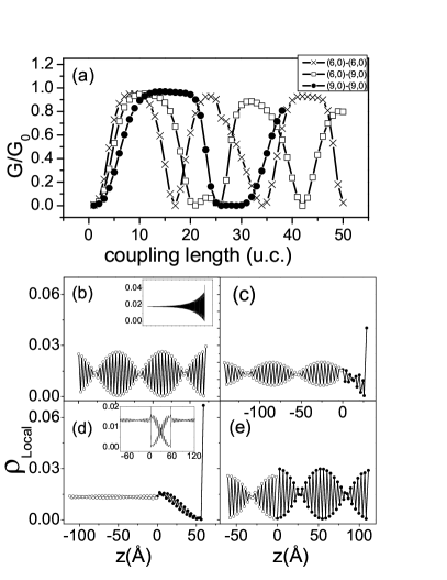
Figure 4: (a) Conductance at E=-0.13eV versus coupling length for (6,0)-(6,0), (6,0)-(9,0) and (9,0)-(9,0) parallel nanotubes respectively. (b)-(e) The LDOS of sites in the coupling line of nanotubes, without coupling, 7, 14 and 27 coupling u.c respectively. The inset of (b) is plotted for a semi-infinite SWNT. The inset of (d) is the LDOS for the whole junction including both left part and right part. We have plotted the LDOS of sites beyond the conductor (hollow circle) for comparison.

The coupling length has significant effects on the conductance. We take a weak coupling value $t_{c}=1.4eV$ to investigate the quantum conductance through the intertube link. As indicated in Figure 4(a), the conductance at E=-0.13eV does not change monotonically with the increasing of coupling length, but shows an oscillating behavior. Starting from the configuration that only one unit cell is connected, the conductance increases with the numbers of coupling unit cells increasing. After reaching a peak value, it decreases and gets a minimum value which is almost zero at certain number of coupling unit cells. When we increase coupling length further, it increases again. The diameters of the two nanotubes are related to the period of oscillations. It needs more coupling length to complete one oscillation for the nanotubes with bigger radii, as illustrated in Figure 4(a). If the coupling length is fixed, the conductance is higher for the nanotubes with bigger radii before reaching the first maximum. The LDOS is a constant at each site for a perfect infinite single-walled carbon nanotube. But for the semi-infinite nanotubes, as shown in figure 4(b), the LDOS at two neighboring sites has a quick oscillation and the envelope has a long period oscillation. The magnitude of envelope oscillation decreases from the end and becomes almost constant far away from the end, as shown in the inset of fig 4(b).

Figure 4(c)-(e) give three typical results of the LDOS in the coupling line. To compare them with each other, we have plotted the LDOS of the same length. The hollow circles are LDOS of the sites at the left lead, and their coordinates are negative. We find that the conductance oscillation behavior is induced by localization and delocalization, which is common in low-dimensional systems, though the mechanism in the current structure is more complicated. The interaction between the electrons in the two nanotubes takes effect through the intertube link. It brings the effective deformation, thus causes the localization of electrons. When high conductance is gotten, the localization disappears and the LDOS have the weakest fluctuations, as in figure 4(d). The LDOS fluctuations in the leads are also weak once the conductance is high. On the contrary, the LDOS have strong fluctuations and the electrons are localized in the conductor region, as shown in figure 4(e).

For 14 u.c. coupling 4(d), the conductance has a high value G=0.97$G_{0}$ since the LDOS has very weak fluctuations. The electrons can transport through the junction easily. The inset of figure 4(d) shows the LDOS of the whole structure including the two nanotubes, electrons have almost entirely transport to the other nanotube at the end. When 26 u.c. was coupled 4(e), the conductance is 0.002$G_{0}$. The electrons are localized in the conductor region and hardly transport through the intertube link, thus the LDOS form strong oscillations in the conductor. Figure 4(c) is the LDOS for 7 coupling u.c. and the corresponding conductance is 0.56$G_{0}$. The magnitude of conductance can be estimated from the LDOS oscillation. The conductance is higher when the oscillations are weaker.

We have also calculated the quantum transport through an infinite metallic zigzag nanotube with an additional finite nanotube nearby, which is placed parallel to the infinite one. The results show that the quantum conductance oscillates too, but within $G_{0}$ and 2 $G_{0}$. The additional part destroys one of the two channels, and the other one is kept unaffected.

IV Summary

We have studied the transport through intertube links between two parallel metallic zigzag SWNTs, using Green’s function method and Landauer formula. It is found that the conductance shows oscillating behaviors. Damped oscillations arise as the coupling strength increases, and the transport gets blocked after a few oscillations. Quantum conductance through the junction also shows oscillations when increasing coupling length. The conductance reaches the maximum which is near 1$G_{0}$ at some coupling length and gets almost zero at some other length. Longer coupling length is needed to finish one oscillation as the radius of nanotube increases. The LDOS has been investigated and the results indicate that the conductance has relation to the amplitudes of the fluctuations of LDOS. When the electrons can transport through the junction with a high (low) conductance, the LDOS shows weak (strong) fluctuations. The electrons in the two semi-infinite nanotubes interfere through the intertube link. These links cause the effective deformation of the nanotubes, which induces the localization and delocalization of the electrons in the conductor. Consequently, the LDOS at the sites of coupling line has weak or strong fluctuations.

A detailed description of the quantum transport through the junction of two parallel zigzag nanotubes is given and further research is needed to achieve a comprehensive understanding in order to construct the pure nanotube-based devices. The work suggests that it should be very careful when constructing devices in nanostructures since the interface or junction is very important for SWNT-based structures. The results implicate that this structure may be utilized to design nanodevices since the intertube transport can be tuned by changing the strength or the length of coupling.

- (1) S. Iijima, Nature (London) 354, 56 (1991).
- (2) R.Saito, G.Dresselhaus, and M.S.Dresselhaus, Physical Properties of Carbon Nanotubes (Imperial College Press, London, 1998).
- (3) S. J. Tans, A. R. M. Verschueren, and C. Dekker, Nature (London), 393, 49 (1998); R. Martel, T. Schmidt, H. R. Shea, T. Hertel, and Ph. Avouris, Appl. Phys. Lett. 73, 2447 (1998).
- (4) M. Bockrath, D. H. Cobden, P. L. McEuen, N. G. Chopra, A. Zettl, A. Thess, and R. E. Smalley, Science 275, 1922, (1997); S. J. Tans, M. H. Devoret, H. Dai, A. Thess, R. E. Smalley, L. J. Geerligs, and C. Dekker, Nature (London) 386, 474 (1997); A. Bachtold, P. Hadley, T. Nakanishi, and C. Dekker, Science 294, 1317 (2001).
- (5) L. Chico, V. H. Crespi, L. X. Benedict, S. G. Louie, and M. L. Cohen, Phys. Rev. Lett. 76, 971 (1996); Z. Yao, H.W. C. Postma, L. Balents, and C. Dekker, Nature (London) 402, 273 (1999).
- (6) T.Rueckes, K. Kim, E. Joslevich, G. Tseng, C. Cheung, and C. M. Lieber, Science 289, 94 (2000).
- (7) S.Datta, Electronic Transport in Mesoscopic System (Cambridge University Press, Cambridge, England, 1995).
- (8) M. F. Yu , T. Kowalewski, R S. Ruoff. Phys. Rev. Lett. 85 1456 (2000).
- (9) M. S. Strano, C.A. Dyke, M. L. Usrey, P. W. Barone, M. J. Allen, H. W. Shan, C. Kitterell, R. H. Hauge, J. M. Tour and R. E. Smalley. Science 301 , 1519 (2003).
- (10) S. Frank, P. Poncharal, Z. L. Wang, W. A. de Heer, Science 280, 1744 (1998).
- (11) S. J. Tans, M. H. Devoret, H. J. Dai, A. Thess, R. E. Smalley, L. J. Geerligs and C. Dekker, Nature (London) 386, 474 (1997); M. Bockrath, D. H. Cobden, P. L. McEuen, N. G. Chopra, A. Zettl, A. Thess and R. E. Smalley, Science 275, 1922 (1997).
- (12) M. Bockrath, D. H. Cobden, J. Lu, A. G. Rinzler, R. E. Smalley, L. Balents and P. L. McEuen, Nature (London) 397, 598 (1999); Yao, Z., Postma, H.W. C., Balents, L. Dekker, C. Nature (London) 402, 273 (1999).
- (13) Y.Q. Xue and M. A. Ratner, Appl. Phys. Lett. 83, 2429 (2003).
- (14) J. Taylor, H. Guo, and J. Wang, Phys. Rev. B 63, 245407 (2001).
- (15) M. Terrones, F. Banhart, N. Grobert, J.C. Charlier, H. Terrones, and P. M. Ajayan, Phys. Rev. Lett. 89, 075505 (2002).
- (16) A. V. Krasheninnikov, K. Nordlund, J. Keinonen, and F. Banhart, Phys. Rev. B 66, 245403 (2002).
- (17) T. Yildirim, O. Gülseren, Ç. Kiliç and S. Ciraci, Phys. Rev. B 62, 12648 (2000).
- (18) M. S. Fuhrer, J. Nygard, L. Shih, M. Forero, Y. G. Yoon, M. S. C. Mazzoni, H. J. Choi, J. Ihm, S. G. Louie, A. Zettl,P. L. McEuen, Nature (London) 288, 494 (2000).
- (19) S. Dag, R.T. Senger, and S. Ciraci, Phys. Rev. B 70, 205407 (2004).
- (20) A. Buldum and J. P. Lu, Appl. Surf. Sci. 215, 123 (2003).
- (21) C. Gómez-Navarro, J. J. Sáenz, and J. Gómez-Herrero, Phys. Rev. Lett.96, 076803 (2006).
- (22) A. Rubio, Appl. Phys. A 68 275 (1999).
- (23) H. F. Song, J. L. Zhu, and J. J. Xiong, Phys. Rev. B 65, 085408 (2002).
- (24) L. Chico, L. X. Benedict, S. G. Louie, and M. L. Cohen, Phys. Rev. B 54, 2600 (1996).
- (25) P. Delaney, H. J. Choi,J. Ihm, S. G. Louie, and M. L. Cohen, Phys. Rev. B 60, 7899 (1999).
- (26) O. Gülseren, T. Yildirim, and S. Ciraci,Phys. Rev. B 65, 153405 (2002).
- (27) V. Zólyomi and J. Kürti, Phys. Rev. B 70, 085403 (2004).
- (28) M. Ouyang, J. L. Huang,C. L. Cheung and C. M. Lieber, Science 292 , 702 (2001).
- (29) J. W. Chen, X. P. Yang L. F. Yang, H. T. Yang and J.M. Dong, Phys. Lett. A 325, 149 (2004).
- (30) M. B. Nardelli, Phys. Rev. B 60, 7828 (1999).