First-order phase transitions in superconducting films: A Euclidean model

Abstract

In the context of the Ginzburg–Landau theory for critical phenomena, we consider the Euclidean $\lambda\phi^{4}+\eta\phi^{6}$ model bounded by two parallel planes, a distance $L$ separating them. This is supposed to describe a sample of a superconducting material undergoing a first-order phase transition. We are able to determine the dependence of the transition temperature $T_{c}$ for the system as a function of $L$. We show that $T_{c}(L)$ is a concave function of $L$, in qualitative accordance with some experimental results. The form of this function is rather different from the corresponding one for a second-order transition.

PACS number(s): 03.70.+k, 11.10.-z

I Introduction

In the last few decades, a large amount of work has been done on the Ginzburg–Landau phenomenological approach to critical phenomena. An account on the state of the subject and related topics can be found, for instance, in Refs. halperin ; affleck ; lawrie1 ; lawrie2 ; brezin ; radzi ; moore ; calan ; malbouisson ; isaque . Questions concerning the existence of phase transitions may also be raised if one considers the behavior of field theories as a function of spatial boundaries. The existence of phase transitions would be in this case associated to some spatial parameters describing the breaking of translational invariance, for instance, the distance $L$ between planes bounding the system. Analyses of this type have been recently performed malbouisson2 ; malbouisson3 ; urucubaca . In particular, if one considers the Ginzburg–Landau model confined between two parallel planes, which is assumed to describe a film of some material, the question of how the critical temperature depends on the film thickness $L$ can be raised.

Studies on field theory applied to bounded systems have been done in the literature for a long time. In particular, an analysis of the renormalization group in finite-size geometries can be found in zinn ; cardy . These have been performed to take into account boundary effects on scaling laws. In another related topic of investigation, there are systems that present domain walls as defects, created for instance in the process of crystal growth by some prepared circumstances. At the level of effective field theories, in many cases, this can be modeled by considering a Dirac fermionic field whose mass changes sign as it crosses the defect, meaning that the domain wall plays the role of a critical boundary separating two different states of the system fosco1 ; fosco2 . Under the assumption that information about general features of the behavior of systems undergoing phase transitions in absence of external influences (like magnetic fields) can be obtained in the approximation which neglects gauge field contributions in the Ginzburg–Landau model, investigations have been done with an approach different from the renormalization group analysis. The system confined between two parallel planes has been considered and using the formalism developed in Refs. malbouisson2 ; malbouisson3 ; urucubaca , the way in which the critical temperature is affected by the presence of boundaries has been investigated. In particular, a study has been done on how the critical temperature $T_{c}$ of a superconducting film depends on its thickness $L$ luciano ; luciano1 ; urucubaca . In the present paper we perform a further step, by considering in the same context an extended model, which besides the quartic field self-interaction, a sextic one is also present. It is well known that those interactions, taken together, lead to a renormalizable quantum field theory in three dimensions and which is supposed to describe first-order phase transitions.

We consider, as in previous publications, that the system is a slab of a material of thickness $L$, the behavior of which in the critical region is to be derived from a quantum field theory calculation of the dependence of the renormalized mass parameter on $L$. We start from the effective potential, which is related to the renormalized mass through a renormalization condition. This condition, however, reduces considerably the number of relevant Feynman diagrams contributing to the mass renormalization, if one wishes to be restricted to first-order terms in both coupling constants. In fact, just two diagrams need to be considered in this approximation: a tadpole graph with the $\phi^{4}$ coupling (1 loop) and a “shoestring” graph with the $\phi^{6}$ coupling (2 loops) (see Fig.1). No diagram with both couplings occur. The $L$-dependence appears from the treatment of the loop integrals, as the material is confined between two planes a distance $L$ apart from one another. We therefore take the space dimension orthogonal to the planes as finite, the other two being otherwise infinite. This dimension of finite extent is treated in the momentum space using the formalism of Ref. malbouisson3 .

The paper is organized as follows. In Section II, we present the model and the description of a bounded system through an adaptation of the Matsubara formalism suited for our purposes. The contributions from the two relevant Feynman diagrams to the effective potential are established, as well as an expression showing the $L$-dependence of the critical temperature. In Section III, as we wish to compare our theoretical result with some experimental data, we need first to make a phenomenological evaluation of the $\phi^{6}$ coupling constant, based on the analogous derivation made by Gorkov for the $\phi^{4}$ constant. The comparison with measurements is discussed in Section IV. Finally, in Section V we present our conclusions.

II The effective potential in the $\phi^{6}$ Ginzburg–Landau model

We start by stating the Ginzburg–Landau Hamiltonian density in a Euclidean $D$-dimensional space, now including both $\phi^{4}$ and $\phi^{6}$ interactions, in the absence of external fields, given by (in natural units, $\hbar=c=k_{B}=1$),

$$\mathcal{H}=\frac{1}{2}\left|\nabla\varphi\right|^{2}+\frac{1}{2}m_{0}^{2}\left|\varphi\right|^{2}-\frac{\lambda}{4}\left|\varphi\right|^{4}+\frac{\eta}{6}\left|\varphi\right|^{6},$$ (1)

where we are taking the approximation in which $\lambda>0$ and $\eta>0$ are the renormalized quartic and sextic self-coupling constants. Near criticality, the bare mass is given by $m_{0}^{2}=\alpha(T/T_{0}-1)$, with $\alpha>0$ and $T_{0}$ being a parameter with the dimension of temperature. Recall that the critical temperature for a first-order transition described by the hamiltonian above is higher than $T_{0}$ lebellac . This will be explicitly stated in Eq. (21) below. We consider the system confined between two parallel planes, normal to the $x$-axis, a distance $L$ apart from one another and use Cartesian coordinates $\mathbf{r}=(x,\mathbf{z})$, where $\mathbf{z}$ is a ($D-1$)-dimensional vector, with corresponding momenta $\mathbf{k}=(k_{x},\mathbf{q}),\mathbf{q}$ being a ($D-1$)-dimensional vector in momenta space. The generating functional of Schwinger functions is written in the form

$$\mathcal{Z}=\int\mathcal{D\varphi}^{*}\mathcal{D\varphi}\exp\left(-\int_{0}^{L}dx\int d^{D-1}z\,\mathcal{H}\left(\left|\varphi\right|,\left|\nabla\varphi\right|\right)\right),$$ (2)

with the field $\varphi(x,\mathbf{z})$ satisfying the condition of confinement along the $x$-axis, $\varphi(x\leq 0,\mathbf{z})=\varphi(x\geq L,\mathbf{z})=$const. Then the field should have a mixed series-integral Fourier representation of the form

$$\varphi(x,\mathbf{z})=\sum_{n=-\infty}^{\infty}c_{n}\int d^{D-1}q\,b(\mathbf{q})e^{-i\omega_{n}x-i\mathbf{q}\cdot\mathbf{z}}\tilde{\varphi}(\omega_{n},\mathbf{q}),$$ (3)

where $\omega_{n}=2\pi n/L$ and the coefficients $c_{n}$ and $b(\mathbf{q})$ correspond respectively to the Fourier series representation over $x$ and to the Fourier integral representation over the ($D-1$)-dimensional $\mathbf{z}$-space. The above conditions of confinement of the $x$-dependence of the field to a segment of length $L$ allow us to proceed, with respect to the $x$-coordinate, in a manner analogous as is done in the imaginary-time Matsubara formalism in field theory and, accordingly, the Feynman rules should be modified following the prescription

$$\int\frac{dk_{x}}{2\pi}\rightarrow\frac{1}{L}\sum_{n=-\infty}^{\infty},\qquad k_{x}\rightarrow\frac{2n\pi}{L}\equiv\omega_{n}.$$ (4)

We emphasize, however, that we are considering an Euclidean field theory in $D$ purely spatial dimensions, so we are not working in the framework of finite-temperature field theory. Here, the temperature is introduced in the mass term of the Hamiltonian by means of the usual Ginzburg–Landau prescription.

To continue, we use some one-loop results described in malbouisson2 ; malbouisson3 ; ananos , adapted to our present situation. These results have been obtained by the concurrent use of dimensional and zeta-function analytic regularizations, to evaluate formally the integral over the continuous momenta and the summation over the frequencies $\omega_{n}$. We get sums of polar ($L$-independent) terms plus $L$-dependent analytic corrections. Renormalized quantities are obtained by subtraction of the divergent (polar) terms appearing in the quantities obtained by application of the modified Feynman rules and dimensional regularization formulas. These polar terms are proportional to $\Gamma$-functions having the dimension $D$ in the argument and correspond to the introduction of counterterms in the original Hamiltonian density. In order to have a coherent procedure in any dimension, those subtractions should be performed even for those values of the dimension $D$ for which no poles are present. In these cases a finite renormalization is performed.

In principle, the effective potential for systems with spontaneous symmetry breaking is obtained, following the Coleman–Weinberg analysis coleman , as an expansion in the number of loops in Feynman diagrams. Accordingly, to the free propagator and to the no-loop (tree) diagrams for both couplings, radiative corrections are added, with increasing number of loops. Thus, at the 1-loop approximation, we get the infinite series of 1-loop diagrams with all numbers of insertions of the $\phi^{4}$ vertex (two external legs in each vertex), plus the infinite series of 1-loop diagrams with all numbers of insertions of the $\phi^{6}$ vertex (four external legs in each vertex), plus the infinite series of 1-loop diagrams with all kinds of mixed numbers of insertions of $\phi^{4}$ and $\phi^{6}$ vertices. Analogously, we should include all those types of insertions in diagrams with 2 loops, etc. However, instead of undertaking this computation, in our approximation we restrict ourselves to the lowest terms in the loop expansion. We recall that the gap equation we are seeking is given by the renormalization condition in which the renormalized squared mass is defined as the second derivative of the effective potential $U(\varphi_{0})$ with respect to the classical field $\varphi_{0}$, taken at zero field,

$$\left.\frac{\partial^{2}U(\varphi_{0})}{\partial\varphi_{0}{}^{2}}\right|_{\varphi_{0}=0}=m^{2}.$$ (5)

Within our approximation, we do not need to take into account the renormalization conditions for the interaction coupling constants, i.e., they may be considered as already renormalized when they are written in the Hamiltonian. At the 1-loop approximation, the contribution of loops with only $\phi^{4}$ vertices to the effective potential is obtained directly from malbouisson3 , as an adaptation of the Coleman–Weinberg expression after compactification in one dimension,

$$U_{1}(\phi,L) = \mu^{D}\sqrt{a}\sum_{s=1}^{\infty}\frac{(-1)^{s+1}}{2s}g_{1}^{s}\phi_{0}^{2s}$$ (6)

$$\times\sum_{n=-\infty}^{\infty}\int\frac{d^{D-1}k}{\left(\mathbf{k}^{2}+an^{2}+c^{2}\right)^{s}}.$$

In the above formula, in order to deal with dimensionless quantities in the regularization procedure, we have introduced parameters $c^{2}=m^{2}/4\pi^{2}\mu^{2}$, $a=(L\mu)^{-2}$, $g_{1}=-\lambda/16\pi^{2}\mu^{4-D}$ and $\phi_{0}=\varphi_{0}/\mu^{D/2-1}$, where $\varphi_{0}$ is the normalized vacuum expectation value of the field (the classical field) and $\mu$ is a mass scale. The parameter $s$ counts the number of vertices on the loop.

It is easily seen that only the $s=1$ term contributes to the renormalization condition (5). It corresponds to the tadpole diagram. It is then also clear that all $\phi^{6}$-vertex and mixed $\phi^{4}$- and $\phi^{6}$-vertex insertions on the 1-loop diagrams do not contribute when one computes the second derivative of similar expressions with respect to the field at zero field: only diagrams with two external legs should survive. This is impossible for a $\phi^{6}$-vertex insertion at the 1-loop approximation, therefore the first contribution from the $\phi^{6}$ coupling must come from a higher-order term in the loop expansion. Two-loop diagrams with two external legs and only $\phi^{4}$ vertices are of second order in its coupling constant, and we neglect them, as well as all possible diagrams with vertices of mixed type. However, the 2-loop shoestring diagram, with only one $\phi^{6}$ vertex and two external legs is a first-order (in $\eta$) contribution to the effective potential, according to our renormalization criterion.

Figure 1: Diagrams contributing to the renormalized mass at lowest order in the coupling constants.

Therefore the renormalized mass is defined at first order in both coupling constants, by the contributions of radiative corrections from only two diagrams: the tadpole and the shoestring diagrams. The tadpole contribution reads (putting $s=1$ in Eq. (6)),

$$U_{1}(\phi_{0},L)=\mu^{D}\sqrt{a}\frac{1}{2}g_{1}\phi_{0}^{2}\sum_{n=-\infty}^{\infty}\int\frac{d^{D-1}k}{\mathbf{k}^{2}+an^{2}+c^{2}}.$$ (7)

The integral on the $D-1$ non-compactified momentum variables is performed using the dimensional regularization formula

$$\int\frac{d^{d}k}{k^{2}+M}=\frac{\Gamma\left(1-\frac{d}{2}\right)\pi^{d/2}}{M^{1-d/2}};$$ (8)

for $d=D-1$, we obtain

$$U_{1}(\phi_{0},L) = \mu^{D}\sqrt{a}\frac{\pi^{(D-1)/2}}{2}g_{1}\phi_{0}^{2}\Gamma\left(\frac{3-D}{2}\right)$$ (9)

$$\times\sum_{n=-\infty}^{\infty}\frac{1}{(an^{2}+c^{2})^{(3-D)/2}}.$$

The sum in the above expression may be recognized as one of the Epstein–Hurwitz zeta-functions, $Z_{1}^{c^{2}}(\frac{3-D}{2};a)$, which may be analytically continued to elizalde

$$Z_{1}^{c^{2}}(\nu;a) = \frac{2^{\frac{2\nu+1}{2}}\pi^{\frac{4\nu-1}{2}}}{\sqrt{a}\Gamma(\nu)}\left[2^{\nu-3/2}\left(\frac{m}{\mu}\right)^{1-2\nu}\Gamma\left(\nu-\frac{1}{2}\right)\right.$$

$$\left.+2\sum_{n=1}^{\infty}\left(\frac{m}{\mu^{2}Ln}\right)^{1/2-\nu}K_{\nu-1/2}(mnL)\right],$$

where the $K_{\nu}$ are Bessel functions of the third kind. The tadpole part of the effective potential is then

$$U_{1}(\phi_{0},L) = \frac{\mu^{D}g_{1}\phi_{0}^{2}}{\left(2\pi\right)^{D/2-2}}\left[2^{-\frac{D+1}{2}}\left(\frac{m}{\mu}\right)^{D-2}\Gamma\left(1-\frac{D}{2}\right)\right.$$

$$\left.+\sum_{n=1}^{\infty}\left(\frac{m}{\mu^{2}Ln}\right)^{D/2-1}K_{D/2-1}(mnL)\right].$$

We now turn to the 2-loop shoestring diagram contribution to the effective potential, using again the Feynman rule prescription for the compactified dimension. It reads

$$U_{2}(\phi,L) = \mu^{2D-2}a\frac{1}{2}g_{2}\phi_{0}^{2}$$

$$\times\left[\Gamma\left(\frac{3-D}{2}\right)\pi^{(D-1)/2}Z_{1}^{c^{2}}\left(\frac{3-D}{2};a\right)\right]^{2},$$

where $g_{2}=\eta/128\pi^{4}\mu^{6-2D}$. After subtraction of the polar term coming from the first term of Eq. (II) we get

$$U_{1}^{\mathrm{(Ren)}}(\varphi_{0},L) = \frac{-\lambda\varphi_{0}^{2}}{4(2\pi)^{D/2}}\sum_{n=1}^{\infty}\left(\frac{m}{\mu^{2}nL}\right)^{D/2-1}K_{D/2-1}(mnL)$$

and

$$U_{2}^{\mathrm{(Ren)}}(\varphi_{0},L) = \frac{\eta\varphi_{0}^{2}}{4(2\pi)^{D}}\left[\sum_{n=1}^{\infty}\left(\frac{m}{nL}\right)^{D/2-1}K_{D/2-1}(mnL)\right]^{2}.$$

Thus the full renormalized effective potential is given by

$$U(\varphi_{0},L)=\frac{1}{2}m_{0}^{2}\varphi_{0}^{2}-\frac{\lambda}{4}\varphi_{0}^{4}+\frac{\eta}{6}\varphi_{0}^{6}+U_{1}^{\text{{(Ren)}}}+U_{2}^{\text{{(Ren)}}}.$$ (15)

The renormalized mass with both contributions then satisfies an $L$-dependent generalized Dyson–Schwinger equation,

$$m^{2}(L) = m_{0}^{2}-\frac{\lambda}{2\left(2\pi\right)^{D/2}}\sum_{n=1}^{\infty}\left(\frac{m}{nL}\right)^{D/2-1}K_{D/2-1}(mnL)$$

$$+\frac{\eta}{4(2\pi)^{D}}$$

$$\times\left[\sum_{n=1}^{\infty}\left(\frac{m}{nL}\right)^{D/2-1}K_{D/2-1}(mnL)\right]^{2}.$$

Thus, the effective potential (15) is rewritten in the form

$$U(\varphi_{0})=\frac{1}{2}m^{2}(L)\varphi_{0}^{2}-\frac{\lambda}{4}\varphi_{0}^{4}+\frac{\eta}{6}\varphi_{0}^{6},$$ (17)

where it is assumed that $\lambda,\eta>0$, a necessary condition for the existence of a first-order phase transition associated to the potential (17). Then, a first-order transition occurs when all the three minima of the potential are simultaneously on the line $U(\varphi_{0})=0$. This gives the condition

$$m^{2}(L)=\frac{3\lambda^{2}}{16\eta}.$$ (18)

Notice that the value $m=0$ is excluded in the above condition, for it corresponds to a second-order transition. For $D=3$, which is the physically interesting situation of the system confined between two parallel planes embedded in a 3-dimensional Euclidean space, the Bessel functions entering in the above equations have an explicit form, $K_{1/2}(z)=\sqrt{\pi}e^{-z}/\sqrt{2z}$, which replaced in Eq.(II), performing the resulting sum, and reminding that $m_{0}^{2}=\alpha(T/T_{0}-1)$, gives

$$m^{2}(L) = \alpha\left(\frac{T}{T_{0}}-1\right)+\frac{\lambda}{8\pi}\frac{1}{L}\ln(1-e^{-m(L)L})$$

$$+\frac{\eta\pi}{8(2\pi)^{3}L^{2}}\left[\ln(1-e^{-m(L)L})\right]^{2}.$$

In Eq.(18) $m(L)$ may have any strictly positive value and this condition ensures that we are on a point on the critical line for a first-order phase transition. Then introducing the value of the mass, Eq.(18), in Eq.(II), we obtain the critical temperature

$$T_{c}(L)=T_{c}\left\{1-\left(1+\frac{3\lambda^{2}}{16\eta\alpha}\right)^{-1}\left[\frac{\lambda}{8\pi\alpha L}\ln(1-e^{-\sqrt{\frac{3\lambda^{2}}{16\eta}}L})+\frac{\eta}{64\pi^{2}\alpha L^{2}}\left(\ln(1-e^{-\sqrt{\frac{3\lambda^{2}}{16\eta}}L})\right)^{2}\right]\right\},$$ (20)

where

$$T_{c}=T_{0}\left(1+\frac{3\lambda}{16\eta\alpha}\right)$$ (21)

is the bulk ($L\rightarrow\infty$) critical temperature for the first-order phase transition.

III Phenomenological evaluation of the constant $\eta$

Our aim in this section is to generalize Gorkov’s gorkov ; abrikosov ; kleinert microscopic derivation done for the $\lambda\varphi^{4}$ model in order to include the additional interaction term $\eta\varphi^{6}$ in the free energy. Here, our interest is to determine the phenomenological constant $\eta$ as a function of the microscopic parameters of the material, in an analogous way as it has been done for the constant $\lambda$ in the $\lambda\varphi^{4}$ model. Using Gorkov’s equations combined with the self-consistent gap condition abrikosov the free energy density may be written in terms of the gap energy $\Delta(x)$ as

$$f(\Delta) = N(0)\left[\xi_{0}^{2}|\nabla\Delta|^{2}+\left(\frac{T}{T_{0}}-1\right)|\Delta|^{2}\right.$$

$$\left.+\frac{3\xi_{0}^{2}}{\hbar^{2}v_{F}^{2}}|\Delta|^{4}+\frac{1674\,\zeta(5)\,\xi_{0}^{4}}{147\,\hbar^{4}v_{F}^{4}\,\zeta^{2}(3)}|\Delta|^{6}\right],$$

where $N(0)$ is the density of states at the Fermi surface, $\xi_{0}$ is the coherence length, $v_{F}$ the Fermi velocity, and $\zeta(x)$ is the Riemann zeta-function. $N(0)$ and $\xi_{0}$ are given by

$$N(0)=\frac{1}{4\pi^{2}k_{B}T_{F}}\left(\frac{p_{F}}{\hbar}\right)^{3}\;,\qquad\xi_{0}\approx 0.13\frac{\hbar v_{F}}{k_{B}T_{0}},$$ (23)

where $T_{F}$ is the Fermi temperature and $k_{B}$ is Boltzmann’s constant. $T_{0}$ is the temperature parameter introduced in Eq. (1) that can be obtained from the first-order bulk critical temperature by means of Eq. (21). Introducing the order parameter $\varphi=\sqrt{2N(0)}\xi_{0}\Delta$ in Eq. (III) we obtain

$$f(\varphi)=\frac{1}{2}|\nabla\varphi|^{2}+\frac{1}{2\xi_{0}^{2}}\left(\frac{T}{T_{0}}-1\right)|\varphi|^{2}+\frac{3}{4\,\hbar^{2}v_{F}^{2}\,\xi_{0}^{2}\,N(0)|}\varphi|^{4}+\frac{1}{6}\frac{1674\,\zeta(5)}{196\,N(0)^{2}\,\hbar^{4}v_{F}^{4}\,\zeta^{2}(3)\,\xi_{0}^{2}}|\varphi|^{6}.$$ (24)

In order to be able to compare our results with some experimental observation, we should restore SI units (remember that so far we have used natural units, $c=\hbar=k_{B}=1$) kleinert . In SI units, the exponent in the partition function (2) has a factor $1/k_{B}T_{0}$. Then, we must divide by $k_{B}T$ the free energy density in Eq. (24). Moreover, we rescale the fields and coordinates by $\varphi_{\text{new}}=\sqrt{\xi_{0}/k_{B}T_{0}}\varphi$ and $x_{\text{new}}=x/\xi_{0}$, which gives the dimensionless energy density and, comparing with Eq. (1), we can identify the phenomenological dimensionless constants $\lambda$, $\eta$, and $m_{0}$, with $\alpha=1$ kleinert ,

$$\lambda\approx 111.08\,\left(\frac{T_{0}}{T_{F}}\right)^{2},\;\;\;\;\eta\approx 0.04257\,\lambda^{2},\;\;\;\;m_{0}^{2}=\frac{T}{T_{0}}-1.$$ (25)

By replacing the above constants in Eq. (20), we get the critical temperature as a function of the film thickness and in terms of microscopic tabulated parameters for specific materials.

IV Comparison with experimental data

We remark that Gorkov’s original derivation of the phenomenological constants is valid only for perfect crystals, where the electron mean free path $l$ is infinite. However, we know that in many superconductors the attractive interaction between electrons (necessary for pairing) is brought about indirectly by the interaction between the electrons and the vibrating crystal lattice (the phonons). Considering that this interaction will be greater if we have impurities within the crystal lattice, consequently the electron mean free path is actually finite. The Ginzburg–Landau phenomenological constants $\lambda$ and $\eta$ and the coherence length are somehow related to the interaction of the electron pairs with the crystal lattice and the impurities. A way of taking these facts into account preserving the form of the Ginzburg–Landau free energy is to modify the intrinsic coherence length and the coupling constants. Accordingly kleinert , $\xi_{0}\rightarrow r^{1/2}\xi_{0}$, $\lambda\rightarrow 2r^{-3/2}\lambda$ and $\eta\rightarrow 4r^{-3}\eta$, where $r\approx 0.18R^{-1}$, with $R=\xi_{0}/l$. Then, Eq. (20) becomes

$$T_{c}(L)=T_{c}\left\{1-\left(1+\frac{3\lambda^{2}}{16\eta}\right)^{-1}\left[\frac{2R\lambda}{0.18\cdot 8\pi}\frac{\xi_{0}}{L}\ln(1-e^{-\frac{L}{\xi_{0}}\sqrt{\frac{3\lambda^{2}}{16\eta}\frac{R}{0.18}}})+\frac{4R^{2}\eta}{0.18^{2}32\pi^{2}}\left(\frac{\xi_{0}}{L}\right)^{2}\left(\ln(1-e^{-\frac{L}{\xi_{0}}\sqrt{\frac{3\lambda^{2}}{16\eta}\frac{R}{0.18}}})\right)^{2}\right]\right\}.$$ (26)

We consider that other effects, such that of the substrate over which the superconductor film is deposited, should be taken into account. In the context of our model, however, we are not able to describe such effects at a microscopic level. We therefore assume that they will be translated in changes on the values of the coupling constants $\lambda$ and $\eta$. So, we propose as an Ansatz the rescaling of the constants in the form $\lambda\rightarrow a\lambda$ and $\eta\rightarrow a^{2}\eta$. We may still combine both parameters $R$ and $a$ as $r=aR$. Eq. (26) is then written as

$$T_{c}(L)=T_{c}\left\{1-\left(1+\frac{3\lambda^{2}}{16\eta}\right)^{-1}\left[\frac{2r\lambda}{0.18\cdot 8\pi}\frac{\xi_{0}}{L}\ln(1-e^{-\frac{L}{\xi_{0}}\sqrt{\frac{3\lambda^{2}}{16\eta}\frac{R}{0.18}}})+\frac{4r^{2}\eta}{0.18^{2}32\pi^{2}}\left(\frac{\xi_{0}}{L}\right)^{2}\left(\ln(1-e^{-\frac{L}{\xi_{0}}\sqrt{\frac{3\lambda^{2}}{16\eta}\frac{R}{0.18}}})\right)^{2}\right]\right\}.$$ (27)

In Fig. 2 we plot Eq. (27) to show the behavior of the transition temperature as a function of the thickness for a film made from aluminum. The values for Al of the Fermi temperature and the bulk critical temperature are $T_{F}=13.53\times 10^{4}$ K and $T_{c}=1.2$ K, respectively.

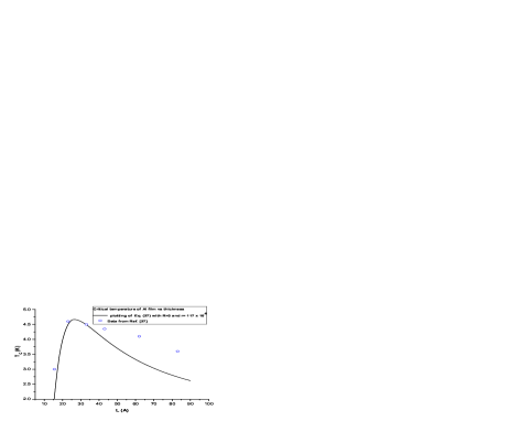
Figure 2: Critical temperature $T_{c}$(K) as function of thickness $L$ ($\AA$), from Eq.(27) and data from Ref. strongin for a superconducting film made from aluminum.

We see from the figure that the critical temperature grows from zero at a nonnull minimal allowed film thickness above the bulk transition temperature $T_{c}$ as the thickness is enlarged, reaching a maximum and afterwards starting to decrease, going asymptotically to $T_{c}$ as $L\rightarrow\infty$. We also plot for comparison some experimental data obtained from Ref. strongin . We see that our theoretical curve is in qualitatively good agreement with measurements, especially for thin films.

The experimental evidence showing that in some superconducting films the transition temperature is well above the bulk one has been reported in the literature since the 1950s and 60s buckel ; strongin2 ; strongin5 ; strongin6 . On the theoretical side, a formula for the transition temperature was written within BCS theory in terms of the electron-phonon coupling constant, the Debye temperature and the Coulomb coupling constant mcmillan . This formula was used to explain observed increases in the critical temperature of thin composite films consisting of alternating layers of dissimilar metals strongin2 . In Ref. dickey a molecular-dynamic technique was applied to obtain the phonon frequency spectrum which led to the same results. Mechanisms accounting for the sharp drop in $T_{c}(L)$ for very thin films were also discussed in Ref. strongin . The authors conclude that the most important influence on $T_{c}(L)$ was the interaction of the film with the substrate, described by a model in Ref. cooper .

It is interesting that in recent reports on copper oxide high-transition-temperature superconductors, the critical temperature depends on the number of layers of CuO₂ in a similar way as above: first it rises with the number of layers and, after reaching a maximum value, then declines. See ramallo and references therein.

This behavior may be contrasted with the one shown by the critical temperature for a second-order transition. In this case, the critical temperature increases monotonically from zero, again corresponding to a finite minimal film thickness, going asymptotically to the bulk transition temperature as $L\rightarrow\infty$. This is illustrated in Fig. 3, adapted from Ref. luciano2 , with experimental data from itoh . (Such behavior has also been experimentally found by some other groups for a variety of transition-metal materials, see Refs. raffy ; minhaj ; pogrebnyakov .) Since in the present work a first-order transition is explicitly assumed, it is tempting to infer that the transition described in the experiments of Ref. strongin is first order. In other words, one could say that an experimentally observed behavior of the critical temperature as a function of the film thickness may serve as a possible criterion to decide about the order of the superconductivity transition: a monotonically increasing critical temperature as $L$ grows would indicate that the system undergoes a second-order transition, whereas if the critical temperature presents a maximum for a value of $L$ larger than the minimal allowed one, this would be signalling the occurrence of a first-order transition.

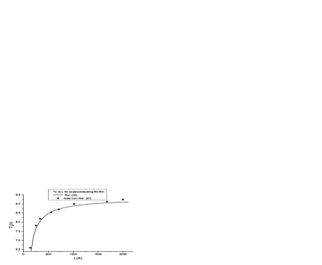
Figure 3: Critical temperature $T_{c}$ (K) as a function of the thickness $L$ ($\AA$) for a second-order transition, as theoretically predicted in Ref. luciano2 . Dots are experimental data taken from Ref. itoh for a superconducting film made from niobium.

V Conclusions

As seen in previous works, a superconducting system confined in some region of space may lose its characteristics if the dimensions of this region become sufficiently small. This is due to the fact that the critical temperature depends on these dimensions in such a way that it vanishes below some finite minimal size. This has been verified in a field-theoretical framework for a Ginzburg–Landau model describing a second-order phase transition. In the present paper, we have studied the critical temperature behavior of a sample of superconducting material in the form of a film, but we have included in the model a $\phi^{6}$ self-interaction term, thus implying that we are now dealing with a first-order transition. In the case we have treated, a sharply contrasting behavior of the critical temperature, as a function of the film thickness, was obtained with respect to the corresponding one for a second-order transition. This possibly indicates a way of discerning the order of a superconducting transition from experimental data, according to the profile of the curve $T_{c}$ vs $L$.

Also importantly, for our derivation of the first-order transition critical temperature curve, we needed to phenomenologically evaluate the $\phi^{6}$ coupling constant, which, as far as we know, is not present in the literature.

Finally, we also remark that in $D=3$, for second-order transitions, one considers $m=0$ and that leads to the need of a pole-subtraction procedure for the mass isaque . In our case such a procedure is not necessary, as a first-order transition must occur for a non-zero value of the mass. This fact, together with the closed formula for the Bessel function for $D=3$, allows us to obtain the exact expression (20) for the critical temperature.

- (1) L. Halperin, T. C. Lubensky, S.-K. Ma, Phys. Rev. Lett. 32, 292 (1974).
- (2) I. Affleck and E. Brézin, Nucl. Phys. 257, 451 (1985).
- (3) I.D. Lawrie, Phys. Rev. B 50, 9456 (1994).
- (4) I.D. Lawrie, Phys. Rev. Lett. 79, 131 (1997).
- (5) E. Brézin, D.R. Nelson and A. Thiaville, Phys. Rev. B 31, 7124 (1985).
- (6) L. Radzihovsky, Phys. Rev. Lett. 74, 4722 (1995).
- (7) M.A. Moore, T.J. Newman, A.J. Bray and S.-K. Chin
- (8) C. de Calan, A.P.C. Malbouisson and F.S. Nogueira, Phys. Rev. B 64, 212502 (2001).
- (9) A.P.C. Malbouisson, F.S. Nogueira and N.F. Svaiter, Eur. Phys. Lett. 41, 547 (1998).
- (10) L.M. Abreu, A.P.C. Malbouisson, I. Roditi, Physica A 331, 99 (2004).
- (11) A.P.C. Malbouisson and J.M.C. Malbouisson, J. Phys. A: Math. Gen. 35, 2263 (2002).
- (12) A.P.C. Malbouisson, J.M.C. Malbouisson and A.E. Santana, Nucl. Phys. B 631, 83 (2002).
- (13) A.P.C. Malbouisson, J.M.C. Malbouisson, A.E. Santana and F.C. Khanna, Mod. Phys. Lett. A 20, 965 (2005).
- (14) J. Zinn-Justin, Quantum Field Theory and Critical Phenomena (Clarendon Press, Oxford, 1996), chapter 36.
- (15) J.L. Cardy (ed.), Finite-Size Scaling (North Holland, Amsterdam, 1988).
- (16) C.D. Fosco and A. Lopez, Nucl. Phys. B 538, 685 (1999).
- (17) L. Da Rold, C.D. Fosco and A.P.C. Malbouisson, Nucl. Phys. B 624, 485 (2002).
- (18) L.M. Abreu, A.P.C. Malbouisson, J.M.C. Malbouisson, A.E. Santana, Phys. Rev. B 67, 212502 (2003).
- (19) A.P.C. Malbouisson, Phys. Rev. B 66, 092502 (2002).
- (20) M. Le Bellac, Quantum and Statistical Field Theory, Oxford University Press, Oxford, 1991.
- (21) G.N.J. Añaños, A.P.C. Malbouisson and N.F. Svaiter, Nucl. Phys. B 547, 221 (1999).
- (22) S. Coleman and E. Weinberg, Phys. Rev. D 7, 1888 (1973).
- (23) A. Elizalde and E. Romeo, J. Math. Phys. 30, 1133 (1989).
- (24) L.P. Gorkov, Sov. Phys. JETP 9, 636 (1959).
- (25) A.A. Abrikosov, L. P. Gorkov, and I. E. Dzyaloshinskii, Methods of Quantum Field Theory in Statistical Physics, 1963.
- (26) H. Kleinert, Gauge Fields in Condensed Matter, Vol. 1: Superflow and Vortex Lines, World Scientific, Singapore, 1989.
- (27) M. Strongin, R.S. Thompson, O.F. Kammerer and J.E. Crow, Phys. Rev. B 1, 1078 (1970).
- (28) V. Buckel and R. Hilsch, Z. Phys. 132, 420 (1952); 138, 109 (1954); N.V. Zavaritsky, Dokl. Akad. Nauk SSSR 86, 501 (1952).
- (29) M. Strongin, O.F. Kammerer, J.E. Crow, R.D. Parks, D.H. Douglass, Jr. and M. A. Jensen, Phys. Rev. Lett. 21, 1320 (1968).
- (30) M. Strongin and O.F. Kammerer, J. Appl. Phys. 39, 2509 (1968).
- (31) M. Strongin, O.F. Kammerer, D.H. Douglass, Jr. and M.H. Cohen, Phys. Rev. Lett. 19 121 (1967).
- (32) W.L. McMillan, Phys. Rev. 167, 331 (1968).
- (33) J.M. Dickey and A. Paskin, Phys. Rev. Lett. 21, 1441 (1968).
- (34) L.N. Cooper, Phys. Rev. Lett. 6, 689 (1961); W. Silvert and L.N. Cooper, Phys. Rev. 141, 336 (1966).
- (35) M.V. Ramallo, Eur. Phys. Lett. 65, 249 (2004); S. Chakravarty, H.-Y. Kee and K. Völker, Nature 428, 53 (2004).
- (36) L.M. Abreu, A.P.C. Malbouisson and I. Roditi, Eur. Phys. J. B 37, 515 (2004).
- (37) J. Kodama, M. Itoh and H. Hirai, J. Appl. Phys., 54, 4050 (1983).
- (38) H. Raffy, R.B. Laibowitz, P. Chaudhari and S. Maekawa, Phys. Rev. B 28, 6607 (1983).
- (39) M.S.M. Minhaj, S. Meepagala, J.T. Chen and L.E. Wenger, Phys. Rev. B 49, 15235 (1994).
- (40) A.V. Pogrebnyakov, J.M. Redwing, J.E. Jones, X.X. Xi, S.Y. Xu, Qi Li, V. Vaithyanathan and D.G. Schlom, Appl. Phys. Lett. 82 (2003) 4319.