Dimensional Control of Antilocalization and Spin Relaxation in Quantum Wires

Abstract

The spin relaxation rate $1/\tau_{s}(W)$ in disordered quantum wires with Rashba and Dresselhaus spin-orbit coupling is derived analytically as a function of wire width $W$. It is found to be diminished when $W$ is smaller than the bulk spin-orbit length $L_{\rm SO}$. Only a small spin relaxation rate due to cubic Dresselhaus coupling $\gamma$ is found to remain in this limit. As a result, when reducing the wire width $W$ the quantum conductivity correction changes from weak anti- to weak localization and from negative to positive magnetoconductivity.

Quantum interference of electrons in low-dimensional, disordered conductors results in corrections to the electrical conductivity $\Delta\sigma$. This quantum correction, the weak localization effect, is known to be a very sensitive tool to study dephasing and symmetry breaking mechanisms in conductorsreview . The entanglement of spin and charge by spin-orbit interaction reverses the effect of weak localization and thereby enhances the conductivity, the weak antilocalization effect. Since the electron momentum is randomized due to disorder, spin-orbit interaction results in randomization of the electron spin, the Dyakonov-Perel spin relaxation with rate $1/\tau_{s}$ perel . This spin relaxation is expected to vanish in narrow wires whose width $W$ is of the order of Fermi wave length $\lambda_{F}$kiselev ; meyer . In this article we show, however, that $1/\tau_{s}$ is already strongly reduced in wider wires: as soon as the wire width $W$ is smaller than bulk spin-orbit length $L_{\rm SO}$. This explains the reduction of spin relaxation rate in n-doped InGaAs-wires, as recently observed with optical holleitner as well as with weak localization measurements hu05 ; gh05 ; schaepers ; lshh04 . There, $L_{\rm SO}$ is as large as several $\mu m$, and exceeds both the elastic mean free path $l_{e}$, and $\lambda_{F}$. In clean, ballistic 2D electron systems (2DES), $L_{\rm SO}$ is the length on which the electron spin precesses a full cycle. It is important to note that this length scale is not changed as the wire width $W$ is reduced below $L_{SO}$, because the spin orbit interaction remains of the same order as in 2D systems. Therefore, this reduction of spin relaxation has the following important consequence: the spin of conduction electrons can precess coherently as it moves along the wire on length scale $L_{SO}$. The spin becomes randomized and relaxes on the longer length scale $L_{s}(W)=\sqrt{D\tau_{s}}$, only ($D=v_{F}^{2}\tau/2$ ($v_{F}$, Fermi velocity) is the 2D diffusion constant). Therefore, the dimensional reduction of spin relaxation rate $1/\tau_{s}(W)$ can be very useful for the realization of spintronic devices, which rely on coherent spin evolutiondasdatta ; spintronics .

Weak antilocalization was predicted by Hikami, Larkin, and Nagaoka nagaoka for conductors with impurities of heavy elements. As conduction electrons scatter from such impurities, the spin-orbit interaction randomizes their spin. The resulting spin relaxation suppresses interference of time reversed paths in spin triplet configurations, while interference in singlet configuration remains unaffected. Since singlet interference reduces the electron’s return probability it enhances the conductivity, the weak antilocalization effect. Weak magnetic fields suppress the singlet contributions, reducing the conductivity and resulting in negative magnetoconductivity. If the host lattice of the electrons provides spin-orbit interaction, quantum corrections to the conductivity have to be calculated in the basis of eigenstates of the Hamiltonian with spin-orbit interaction,

$$H_{0}=(\hbar^{2}/2m_{e}){\bf k^{2}}+\hbar\mbox{\boldmath$\sigma$}{\bf\Omega},$$ (1)

($m_{e}$, effective electron mass), ${\bf\Omega}^{T}=(\Omega_{x},\Omega_{y})$, are precession frequencies of the electron spin around the x- and y-axis. $\sigma$ is a vector, with components $\sigma_{i}$, $i=x,y$, the Pauli matrices. The breaking of inversion symmetry causes a spin-orbit interaction, given by dresselhaus

$${\bf\Omega_{D}}=\alpha_{1}(-\hat{e}_{x}k_{x}+\hat{e}_{y}k_{y})/\hbar+\gamma(\hat{e}_{x}k_{x}k_{y}^{2}-\hat{e}_{y}k_{y}k_{x}^{2})/\hbar.$$ (2)

$\alpha_{1}=\gamma\langle k_{z}^{2}\rangle$, the linear Dresselhaus parameter, measures the strength of the term linear in momenta $k_{x},k_{y}$ in the plane of the 2DES. When $\langle k_{z}^{2}\rangle\sim 1/a^{2}\geq k_{F}^{2}$ ($a$, thickness of the 2DES, $k_{F}$, Fermi wave number), that term exceeds the cubic Dresselhaus terms with coupling $\gamma$. Asymmetric confinement of the 2DES yields the Rashba term ($\alpha_{2}$,Rashba parameter) rashba ,

$${\bf\Omega_{R}}=\alpha_{2}(\hat{e}_{x}k_{y}-\hat{e}_{y}k_{x})/\hbar.$$ (3)

The quantum correction to the conductivity $\Delta\sigma$ arises from the fact, that the quantum return probability to a given point ${\bf x_{0}}$ after a time $t$, $P(t)$, differs from the classical return probability, due to quantum interference. Therefore, $\Delta\sigma$ is proportional to a time integral over the quantum mechanical return probability $P(t)=\lambda_{F}^{d}(t)n({\bf x_{0}},t)$ ($d$, dimension of diffusion, $n$, electron density). For uncorrelated disorder potential, $V(x)$, with $\langle V\rangle=0$ and $\langle V(x)V(x^{\prime})\rangle=\delta(x-x^{\prime})/2\pi\nu\tau$ ($\nu=m/(2\pi\hbar^{2})$, average density of states per spin channel, $\tau$, elastic mean free time), we can perform the disorder average. Going to momentum (${\bf Q}$) and frequency ($\omega$) representation, and summing up ladder diagrams to take into account the diffusive motion, yields the quantum correction to the static conductivity nagaoka ,

$$\Delta\sigma=-\frac{2e^{2}}{h}\frac{\hbar D}{Vol.}\sum_{\bf Q}\sum_{\alpha,\beta=\pm}C_{\alpha\beta\beta\alpha,\omega=0}({\bf Q}),$$ (4)

where $\alpha,\beta=\pm$ are the spin indices, and the Cooperon propagator $\hat{C}$ is for $\epsilon_{F}\tau\gg 1$ ( $\epsilon_{F}$, Fermi energy), and neglecting the Zeeman coupling,

$$\hat{C}({\bf Q})^{-1} = \frac{\hbar}{\tau}-\int\frac{d\Omega}{\Omega}\frac{\hbar/\tau}{1+i\frac{\tau}{\hbar}{\bf v}(\hbar{\bf Q}+2e{\bf A}+2m_{e}\hat{a}{\bf S})}.$$ (5)

The integral is over all angles of velocity ${\bf v}$ on the Fermi surface ($\Omega$, total angle. $e$, electron charge, ${\bf A}$, vector potential). ${\bf S}$ is the total spin vector of spins of time reversed paths: ${\bf S}=\left(\mbox{\boldmath$\sigma$}+\mbox{\boldmath$\sigma$}^{\prime}\right)/2$. $\hat{a}$ is the 2 by 2 matrix

$$\hat{a}=\frac{1}{\hbar}\left(\begin{array}[]{cc}-\alpha_{1}+\gamma k_{y}^{2}&-\alpha_{2}\\ \alpha_{2}&\alpha_{1}-\gamma k_{x}^{2}\end{array}\right).$$ (6)

In 2D, the angular integral is continuous from $0$ to $2\pi$, yielding to lowest order in $({\bf Q}+2e{\bf A}+2m\hat{a}{\bf S})$,

$$\hat{C}({\bf Q})=\frac{\hbar}{D(\hbar{\bf Q}+2e{\bf A}+2e{\bf A}_{\bf S})^{2}+H_{\gamma}}.$$ (7)

The effective vector potential due to spin-orbit interaction, ${\bf A}_{\bf S}=m_{e}\hat{\alpha}{\bf S}/2$, ($\hat{\alpha}=\langle\hat{a}\rangle$) couples to total spin ${\bf S}$. The cubic Dresselhaus coupling reduces the effect of the linear one to $\alpha_{1}-m_{e}\gamma\epsilon_{F}/2$. Furthermore, it gives rise to the spin relaxation term in Eq. (7),

$$H_{\gamma}=D\frac{m_{e}^{2}\epsilon_{F}^{2}\gamma^{2}}{\hbar^{2}}(S_{x}^{2}+S_{y}^{2}).$$ (8)

In the representation of the singlet, $\mid~{}S=0;m=0\rangle$ and triplet states $\mid~{}S=1;m=0,\pm\rangle$, $\hat{C}$ decouples into a singlet and a triplet sector. Thus, the quantum conductivity is a sum of singlet and triplet terms,

$$\Delta\sigma = -2\frac{e^{2}}{h}\frac{\hbar D}{Vol.}\sum_{\bf Q}\left(-\frac{\hbar}{D(\hbar{\bf Q}+2e{\bf A})^{2}}\right.$$ (9)

$$\left.+\sum_{m=0,\pm 1}\langle S=1,m\mid\hat{C}({\bf Q})\mid S=1,m\rangle\right).~{}~{}~{}~{}~{}$$

The triplet terms have been evaluated in various approximations beforeknap ; miller ; af01 ; lg98 ; golub . In 2D one can treat the magnetic field nonperturbatively, using the basis of Landau bandsnagaoka . In wires with widths smaller than cyclotron length $k_{F}l_{B}^{2}$ ($l_{B}$, the magnetic length, defined by $Bl_{B}^{2}=\hbar/e$), the Landau basis is not suitable. Fortunately, there is another way to treat magnetic fields: quantum corrections are due to the interference between closed time reversed paths. In magnetic fields the electrons acquire a magnetic phase, which breaks time reversal invariance. Averaging over all closed paths, one obtains a rate with which the magnetic field breaks the time reversal invariance, $1/\tau_{B}$. Like the dephasing rate $1/\tau_{\varphi}$, it cuts off the divergence arising from quantum corrections with small wave vectors ${\bf Q}^{2}<1/D\tau_{B}$. In 2D systems, $\tau_{B}$ is the time an electron diffuses along a closed path enclosing one magnetic flux quantum, $D\tau_{B}=l_{B}^{2}$. In wires of finite width $W$ the area which the electron path encloses in a time $\tau_{B}$ is $W\sqrt{D\tau_{B}}$. Requiring that this encloses one flux quantum gives $1/\tau_{B}=De^{2}W^{2}B^{2}/(3\hbar^{2})$. For arbitrary magnetic field the relation $1/\tau_{B}=D(2e)^{2}B^{2}\langle y^{2}\rangle/\hbar^{2}$ with the expectation value of the square of the transverse position $\langle y^{2}\rangle$, yields $1/\tau_{B}=D/l_{B}^{2}\left(1-1/(1+W^{2}/3l_{B}^{2})\right)$. Thus, it is sufficient to diagonalize the Cooperon propagator as given by Eq.(7) without magnetic field and to add the magnetic rate $1/\tau_{B}$ together with dephasing rate $1/\tau_{\varphi}$ to the denumerator of $\hat{C}({\bf Q})$, when calculating the conductivity correction, Eq. (9).

It is well known that the Cooperon propagator can be diagonalized in 2D for pure Rashba coupling $\alpha_{1}=0,\gamma=0$, or pure Dresselhaus coupling $\alpha_{2}=0$iordanskii ; knap ; lg98 ; golub . For example, keeping only Rashba coupling $\alpha_{2}$ the three triplet Cooperon Eigenvalues are in 2D,

$$E_{T0}/(D\hbar)={\bf Q}^{2}+Q_{SO}^{2},$$

$$E_{T\pm}/(D\hbar)={\bf Q}^{2}+\frac{3}{2}Q_{SO}^{2}\pm\frac{1}{2}Q_{SO}^{2}\sqrt{1+16\frac{{\bf Q}^{2}}{Q_{SO}^{2}}},~{}~{}~{}~{}~{}$$ (10)

where $Q_{SO}=2m_{e}\alpha_{2}/\hbar^{2}$. If we use the approximation,

$$E_{T\pm}/(D\hbar)\approx(Q\pm Q_{SO})^{2}+Q_{SO}^{2}/2,$$ (11)

which is plotted for comparison with the exact dispersion, Eq. (Dimensional Control of Antilocalization and Spin Relaxation in Quantum Wires) in Fig. 1, we can integrate analytically over the 2D momenta. Thus, the 2D quantum correction is

$$\Delta\sigma=-\frac{1}{2\pi}\ln\frac{H_{\varphi}}{H_{\varphi}+H_{s}}+\frac{1}{\pi}\ln\frac{H_{\varphi}+H_{s}/2}{H_{\tau}},$$ (12)

in units of $e^{2}/h$. All parameters are rescaled to dimensions of magnetic fields: $H_{\varphi}=\hbar/(4eD\tau_{\varphi})$, $H_{\tau}=\hbar/(4eD\tau)$, and the spin relaxation field $H_{s}=\hbar/(4eD\tau_{Sxx})$knap . The 2D spin relaxation rate of one spin component is for pure Rashba coupling, $1/\tau_{Sxx}=1/\tau_{s}=2p_{F}^{2}\alpha_{2}^{2}\tau$ knap ; iordanskii , and is related to spin-orbit gap $\Delta_{SO}=\hbar v_{F}Q_{SO}$, by $1/\tau_{s}=(\Delta_{SO}/\hbar)^{2}\tau/d$.

Note that the magnetoconductivity is dominated by the minima of the dispersion of Cooperon eigenvalues. Therefore, these minima, whose finite value we may call spin relaxation gaps, are a direct measure of spin relaxation rate. We note that the lowest minima of the triplet modes are shifted to nonzero wave vectors, $Q=\pm Q_{SO}$. Thus, the spin relaxation gap is by about a factor $1/2$ smaller, than at $Q=0$ iordanskii .

Without spin-orbit interaction, the conductivity of quantum wires with width $W<L_{\varphi}$ is dominated by the transverse zero mode $Q_{y}=0$. This yields the quasi-1D weak localization correction as used previously for narrow GaAs wireskurdak . However, in the presence of spin-orbit interaction, setting simply $Q_{y}=0$ is not correct. Rather one has to solve the Cooperon equation with the modified boundary conditionsaf01 ; meyer ,

$$(-i\partial_{y}+2eA_{Sy})C(x,y=\pm W/2)=0,$$ (13)

for all $x$.

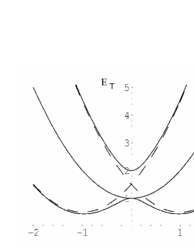
Figure 1: Dispersion of triplet Cooperon modes in 2D in units of $\hbar DQ_{SO}^{2}$, Eqs. (Dimensional Control of Antilocalization and Spin Relaxation in Quantum Wires) (full lines), and Eq. (11) (dashed lines).

The transverse zero mode $Q_{y}=0$ does not satisfy this condition. Therefore, it is convenient to perform a Non-Abelian gauge transformation af01 . Since in quantum wires these boundary conditions apply only in the transverse direction, a transformation in the transverse direction is needed, only: $\hat{C}\rightarrow\tilde{C}=U\hat{C}\bar{U}$, with $U=\exp(i2eA_{Sy}y/\hbar)$. Then, the boundary condition simplifies to, $-i\partial_{y}\tilde{C}(x,y=\pm W/2)~{}=~{}0$. For $W<L_{\varphi}$ we can use the fact that transverse nonzero modes contribute terms to the conductivity which are a factor $W/nL_{\varphi}$ smaller than the 0-mode term, with $n$ a nonzero integer number. Therefore, it is sufficient to diagonalize the effective quasi-1-dimensional Cooperon propagator: the transverse 0-mode expectation value of the transformed inverse Cooperon propagator $\tilde{H}_{1D}=\langle 0\mid\tilde{C}^{-1}\mid 0\rangle$. It is crucial to note that additional terms are created in $\tilde{H}_{1D}$ by the non-Abelian transformation. We can diagonalize $\tilde{H}_{1D}$, neglecting small relaxation due to cubic Dresselhaus coupling $\gamma$. We introduce the notation, $Q_{SO}^{2}=Q_{D}^{2}+Q_{R}^{2}$ where $Q_{D}$ depends on Dresselhaus spin-orbit coupling, $Q_{D}=m_{e}(2\alpha_{1}-m_{e}\epsilon_{F}\gamma)/\hbar$. $Q_{R}$ depends on Rashba coupling: $Q_{R}=2m_{e}\alpha_{2}/\hbar$. We finally find the dispersion of quasi-1D triplet modes,

$$\frac{E_{T0}}{\hbar D}=Q_{x}^{2}+Q_{SO}^{2}\delta_{SO}^{2}\left(\frac{1}{2}t_{SO}\delta_{SO}^{2}+2c_{SO}(1-\delta_{SO}^{2})\right),$$

$$\frac{E_{T\pm}}{\hbar D}=Q_{x}^{2}+\frac{1}{4}Q_{SO}^{2}\left(4-t_{SO}\delta_{SO}^{4}-4c_{SO}\delta_{SO}^{2}(1-\delta_{SO}^{2})\right.$$

$$\left.\pm 2\sqrt{h(\delta_{SO})+\frac{16Q_{x}^{2}}{Q_{SO}^{2}}(1+c_{SO}(c_{SO}-2)\delta_{SO}^{2})}\right),$$ (14)

where $\delta_{SO}=(Q_{R}^{2}-Q_{D}^{2})/Q_{SO}^{2}$, and

$$c_{SO}=1-\frac{2\sin(Q_{SO}W/2)}{Q_{SO}W},~{}t_{SO}=1-\frac{\sin(Q_{SO}W)}{Q_{SO}W}.$$ (15)

Here, $h(\delta_{SO})=t_{SO}\delta_{SO}^{8}/4+\delta_{SO}^{2}(1-\delta_{SO}^{2})(4c_{SO}^{2}(1-3\delta_{SO}^{2}+3\delta_{SO}^{4})+t_{SO}^{2}\delta_{SO}^{2}(1+\delta_{SO}^{2})-6c_{SO}t_{SO}\delta_{SO}^{4})$. In Fig. 2, the gap of $E_{T0}$ and the full dispersion of the other two triplet modes are plotted for pure Rashba coupling $\delta_{SO}=1$, as a function of the wire width $W$ as scaled with $Q_{SO}$. In Fig. 3 the magnetoconductivity is plotted for pure Rashba coupling $\delta_{SO}=1$ as function of the wire width $W$. Inserting Eq. (Dimensional Control of Antilocalization and Spin Relaxation in Quantum Wires) into the expression for the quantum correction to the conductivity Eq. (9), the integral over momentum $Q_{x}$ is done numerically. We note a change of sign from weak antilocalization to weak localization as $Q_{SO}W$ becomes smaller than 1. In the crossover regime $Q_{SO}W\approx 1$ very weak magnetoconductivity is found.

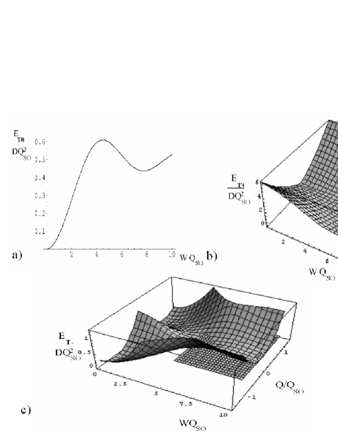
Figure 2: For pure Rashba coupling $\delta_{SO}=1$: a) Gap of Triplet mode $E_{T0}$ as function of wire width $W$ (in units of $L_{SO}=1/Q_{SO}$). b) Dispersion of Triplet mode $E_{T+}$ and c) of $E_{T-}$ as function of width $W$ and momentum $Q$ (scaled with $Q_{SO}$) and $E/(\hbar DQ_{SO}^{2})=1/2$ for comparison.

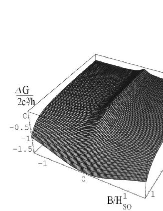
Figure 3: The quantum conductivity correction in units of $2e^{2}/h$ as function of magnetic field $B$ (scaled with bulk relaxation field $H_{s}$), and the wire width $W$ (scaled with spin-orbit length $L_{SO}$), for pure Rashba coupling, $\delta_{SO}=1$.

In the limit $WQ_{SO}\gg 1$ the gaps of the triplet mode dispersions given in Eq. (Dimensional Control of Antilocalization and Spin Relaxation in Quantum Wires) coincide with the 2D gap values $\hbar DQ_{SO}^{2}(1/2,1/2,1)$ of Eqs. (Dimensional Control of Antilocalization and Spin Relaxation in Quantum Wires) (Note that the spin quantization axis is rotated by the unitary transformation). For $WQ_{SO}<1$ the spin-orbit gap of the triplet mode $E_{T0}$ is to first order in $t_{SO}$ and $c_{SO}$ given by $\Delta_{0}=DQ_{SO}^{2}(2c_{SO}\delta_{SO}^{2}(1-\delta_{SO}^{2})+t_{SO}\delta_{SO}^{4}/2)$ and the gap of $E_{T\pm}$ is $\Delta_{\pm}=\Delta_{0}/2+DQ_{SO}^{2}(2c_{SO}-t_{SO}/2)\delta_{SO}^{4}$. Thus, for $WQ_{SO}\ll 1$ the weak localization correction is

$$\Delta\sigma=\frac{\sqrt{H_{W}}}{\sqrt{H_{\varphi}+B^{*}(W)/4}}-\frac{\sqrt{H_{W}}}{\sqrt{H_{\varphi}+B^{*}(W)/4+H_{s}(W)}}$$

$$-2\frac{\sqrt{H_{W}}}{\sqrt{H_{\varphi}+B^{*}(W)/4+H_{s}(W)/2}},$$ (16)

in units of $e^{2}/h$. We defined $H_{W}=\hbar/(4eW^{2})$, and the effective external magnetic field,

$$B^{*}(W)=(1-1/(1+\frac{W^{2}}{3l_{B}^{2}}))B.$$ (17)

The spin relaxation field $H_{s}(W)$ is for $W<L_{SO}$,

$$H_{s}(W)=\frac{1}{12}(\frac{W}{L_{SO}})^{2}\delta_{SO}^{2}H_{s},$$ (18)

suppressed in proportion to $(W/L_{SO})^{2}$. The analogy to the effective magnetic field, Eq. (17), could be expected, since the spin orbit coupling enters the Cooperon, Eq. (7), like an effective magnetic vector potentialfalko . Cubic Dresselhaus coupling gives rise to an additional spin relaxation term, Eq. (8), which has no analogy to a magnetic field and is therefore not suppressed. When $W$ is larger than spin-orbit length $L_{SO}$, coupling to higher transverse modes becomes relevantaleiner . One can expect that in ballistic wires, $l_{e}>W$, the spin relaxation rate is suppressed in analogy to the flux cancellation effect, which yields the weaker rate, $1/\tau_{s}=(W/Cl_{e})(DW^{2}/12L_{SO}^{4})$, where $C=10.8$km02 .

In conclusion, in wires whose width $W$ is smaller than bulk spin orbit length $L_{SO}$ spin relaxation due to linear Rashba and Dresselhaus spin-orbit coupling is suppressed. The spin relaxes then due to small cubic Dresselhaus coupling, only. Thus, the total spin relaxation rate as function of wire width is for $W<L_{SO}$,

$$\frac{1}{\tau_{s}}(W)=\frac{1}{12}(\frac{W}{L_{SO}})^{2}\delta_{SO}^{2}\frac{1}{\tau_{s}}+D\frac{(m_{e}^{2}\epsilon_{F}\gamma)^{2}}{\hbar^{3}},$$ (19)

where $1/\tau_{s}=2p_{F}^{2}(\alpha_{2}^{2}+(\alpha_{1}-m_{e}\gamma\epsilon_{F}/2)^{2})\tau$. The enhancement of spin relaxation length $L_{s}=\sqrt{D\tau_{s}(W)}$ can be understood as follows: The area an electron covers by diffusion in time $\tau_{s}$ is $WL_{s}$. This should be equal to the corresponding 2D area $L_{SO}^{2}$ falko , which yields $1/L_{s}^{2}\sim(W/L_{SO})^{2}/L_{SO}^{2}$, in agreement with Eq. (18). At lower temperatures, when dephasing length $L_{\varphi}$ exceeds $L_{\gamma}=\hbar/m_{e}^{2}\epsilon_{F}\gamma$, a weak antilocalization peak is recovered at small magnetic fields, $l_{B}>L_{\gamma}$. Reduction of spin relaxation has recently been observed in optical measurements of n-doped InGaAs quantum wiresholleitner , where $\delta_{SO}\approx 1$, and in transport measurementshu05 ; gh05 , and also in GaAs wireslshh04 . Ref. holleitner reports saturation of spin relaxation in narrow wires, $W\ll L_{SO}$, attributed to cubic Dresselhaus coupling, in full agreement with Eq. (19).

We thank V. L. Fal’ko, and F. E. Meijer for stimulating discussions, I. Aleiner, C. Marcus, T. Ohtsuki, K. Slevin, K. Dittmer, J. Ohe, and A. Wirthmann for helpful discussions, and A. Chudnovskiy, K. Patton and E. Mucciolo for useful comments. We gratefully acknowledge the hospitality of MPIPKS in Dresden, the Physics Department of Sophia University, Tokyo and Aspen Center for Physics. This work was supported by SFB508 B9.

References

- (1) B. L. Altshuler, A. G. Aronov, D. E. Khmelnitskii, and A. I. Larkin, in Quantum Theory of Solids, edited by I. M. Lifshits (Mir, Moscow, 1982); G. Bergmann, Phys. Rep. 107, 1 (1984); S. Chakravarty, A. Schmid, Phys. Rep. 140, 193 (1986).
- (2) M. I. D’yakonov and V. I. Perel’, Sov. Phys. Solid State 13, 3023 (1972).
- (3) A. A. Kiselev, and K. W. Kim, Phys. Rev. B 61, 13115 (2000).
- (4) J. S. Meyer, V. I. Fal’ko, B.L. Altshuler, Nato Science Series II, 72, 117, ed. I.V. Lerner, B.L. Altshuler, V.I. Fal’ko, and T. Giamarchi (Kluwer Academic Publishers, Dordrecht, 2002).
- (5) A. W. Holleitner, V. Sih, R. C. Myers, A. C. Gossard, D. D. Awschalom, Phys. Rev. Lett. 97, 036805 (2006).
- (6) A. Wirthmann, Y. S. Gui, C. Zehnder, C. Heyn, D. Heitmann,C. -M. Hu, and S. Kettemann, Physica E 34, 493 (2006).
- (7) F. E. Meijer, private communication (2005).
- (8) Th. Schäpers, V. A. Guzenko, M. G. Pala, U. Zülicke, M. Governale, J. Knobbe, and H. Hardtdegen Phys. Rev. B 74, 081301(R) (2006).
- (9) R. Dinter, S. Löhr, S. Schulz, Ch. Heyn, and W. Hansen, unpublished (2005).
- (10) B. Datta and S. Das, Appl. Phys. Lett. 56, 665 (1990).
- (11) I. Zutic’, J. Fabian, and S. Das Sarma Rev. Mod. Phys. 76, 323 (2004).
- (12) S. Hikami, A. I. Larkin, and Y. Nagaoka, Prog. Theor. Phys. 63 , 707 (1980).
- (13) G. Dresselhaus, Phys. Rev. 100, 580(1955).
- (14) E. I. Rashba, Fiz. Tverd. Tela (Leningrad) 2, 1224 (1960) [Sov. Phys. Solid State 2, 1109 (1960)]; Yu. A. Bychkov and E. I. Rashba, Pis’ma Zh. Eksp. Teor. Fiz. 39, 66 (1984).
- (15) W. Knap, C. Skierbiszewski, A. Zduniak, E. Litwin-Staszewska, D. Bertho, F. Kobbi, J. L. Robert, G. E. Pikus, F. G. Pikus, S. V. Iordanskii, V. Mosser, K. Zekentes, and Yu. B. Lyanda-Geller, Phys. Rev. B 53, 3912 (1996).
- (16) J. B. Miller, D.M. Zumbuhl, C.M. Marcus, Y.B. Lyanda-Geller, D. Goldhaber-Gordon, K. Campman, and A.C. Gossard, Phys. Rev. Lett. 90, 076807 (2003).
- (17) Y. Lyanda-Geller, Phys. Rev. Lett. 80, 4273 (1998).
- (18) L. E. Golub, Phys. Rev. B 71, 235310 (2005).
- (19) I. L. Aleiner, V. I. Fal’ko, Phys. Rev. Lett. 87, 256801 (2001).
- (20) S. V. Iordanskii, Yu. B. Lyanda-Geller, and G. E. Pikus, JETP Lett. 60, 206 (1994).
- (21) C. Kurdak, A. M. Chang, A. Chin, and T. Y. Chang, Phys Rev. B 46, 6846 (1992).
- (22) V. L. Fal’ko, private communication, (2003).
- (23) I. L. Aleiner, privtate communication (2006).
- (24) V. K. Dugaev, D. E. Khmeln’itskii, JETP 59, 1038 (1984); C. W. J. Beenakker and H. van Houten, Phys. Rev. B 37, 6544 (1988); S. Kettemann and R. Mazzarello, Phys. Rev. B 65, 085318 (2002).